Dimension Estimation Using Random Connection Models
Paulo Serra∗ [email protected]
Department of Mathematics and Computer Science Groene Loper 5
MetaForum Building
Eindhoven University of Technology 5612 AZ Eindhoven, the Netherlands
Michel Mandjes [email protected]
Korteweg-de Vries Institute for Mathematics Science Park 105–107
University of Amsterdam
1098 XG Amsterdam, the Netherlands
Editor:Franc¸ois Caron
Abstract
Information about intrinsic dimension is crucial to perform dimensionality reduction, com-press information, design efficient algorithms, and do statistical adaptation. In this paper we propose an estimator for the intrinsic dimension of a data set. The estimator is based on binary neighbourhood information about the observations in the form of two adjacency matrices, and does not require any explicit distance information. The underlying graph is modelled according to a subset of a specific random connection model, sometimes referred to as the Poisson blob model. Computationally the estimator scales like nlogn, and we specify its asymptotic distribution and rate of convergence. A simulation study on both real and simulated data shows that our approach compares favourably with some competing methods from the literature, including approaches that rely on distance information.
Keywords: adaptation, dimensionality reduction, intrinsic dimension, random connec-tion model, random graph
1. Introduction
In machine learning and computational geometry we often want to discover, or sometimes impose, structure on observations, and dimension plays a crucial role in this task. The dimension of a data set can perhaps be best interpreted as the number of variables needed to describe it. However, there is often a gap between the ambient dimension of a data set – the number of variablesusedto describe it – and its intrinsic dimension – the number of variables
needed to describe it (eventually up to a certain level of precision). For instance, high-dimensional data sets often live in lower high-dimensional spaces; infinite-high-dimensional parameters of non-parametric models can often be accurately estimated using just a few parameters; complex data can potentially be highly compressible. However, this is usually not evident by
∗. This research took place while this author was a postdoctoral researcher at the Korteweg-de Vries Institute for Mathematics, of the University of Amsterdam, in Amsterdam, the Netherlands.
c
just looking at the data, so in this paper we propose an algorithm to estimate the intrinsic dimension of a data set, and study its behaviour.
There are plenty of reasons to be interested in intrinsic dimensions. Perhaps the most straightforward one is to perform dimensionality reduction. Dimensionality reduction arises from a need to be able to extract meaningful conclusions from high-dimensional observa-tions. There is an extensive literature on this subject using multidimensional scaling, man-ifold learning, and projection techniques like principal component analysis and projection pursuit; for a general overview cf. (Fodor, 2002; Burges, 2010; Lee and Verleysen, 2007). For specific techniques see for example (Kohonen, 1990; Cox and Cox, 2000; Tenenbaum et al., 2000; Roweis and Saul, 2000; Donoho and Grimes, 2003; Huo and Chen, 2002; Gin´e and Koltchinskii, 2006), and the references therein. In order to be used to their full extent, these approaches require a priori knowledge about the intrinsic dimension of the data set. Knowledge about intrinsic dimension is also important in independent component analysis; cf. (Hyviirinen et al., 2001).
From a statistical perspective, the intrinsic dimension provides information about the difficulty of making inference. Non-parametric estimators usually rely on approximation properties of certain function spaces; the dimension of the support of these functions influ-ences these approximation properties. Statistical adaptation often focuses on smoothness, but dimension actually has a more substantial impact on rates of convergence. Knowledge about dimension is also important to avoid (if possible) the curse of dimensionality. Dimen-sion plays an important role in classification problems as well, where performance is greatly compromised in high dimensions; cf. (Bickel and Levina, 2004; Fan and Fan, 2008). There are also connections to search, and to outlier detection; cf. (Amsaleg et al., 2015) and the references therein.
From a computational perspective, the dimension of a data set impacts the amount of space needed to store data (compressibility). The speed of algorithms is also commonly af-fected by the dimension of input data. Learning the underlying dimension is also important to design algorithms that require less data (meaning, make better use of available data) when data happen to live on a low dimensional space. Because of this, knowledge about dimension is crucial in many fields such as biomedicine, economics, engineering, astronomy, remote sensing, and computer vision, with important applications in mass spectrometry, genetics, networking, image processing, automatic text analysis, among others; for some concrete applications see (Verleysen et al., 1999; L¨ahdesm¨aki et al., 2005; Abrahao and Kleinberg, 2008; Carter et al., 2010) and references therein.
More recent work of (Camastra and Vinciarelli, 2002; K´egl, 2002; Hein and Audibert, 2005; Sricharan et al., 2010) is based on the notion of correlation integral; cf. (Grassberger and Procaccia, 2004). The correlation dimension is a limit associated with this correlation integral. This notion of dimension, which we also use in this paper, is computationally attractive when compared with other notions of dimension such as that of box counting dimension, for example. There are also the techniques of (Costa and Hero, 2004; Farahmand et al., 2007; Leonenko et al., 2008; Kleindessner and von Luxburg, 2015) based on different types of graphs where edges represent some form of proximity, like k-nearest neighbour graphs, and geodesic minimal spanning trees. Their work relies on the fact that certain quantities associated with these graphs scale monotonically with dimension. By exploring this, one can extract information about dimensionality by inverting these relations. A similar idea is used in (Amsaleg et al., 2015) by recurring to notions from extreme value theory. See also (Eriksson and Crovella, 2012) for a clustering-based approach, and the work of (Levina and Bickel, 2004) for an estimator based on an approximation of the likelihood. There is some room for improvement in the approaches mentioned above. Some of them rely on rather extensive knowledge about distances between all possible pairs of ob-servations, sometimes also of perturbations thereof, or on certain hierarchical constructs like dendrograms; because execution times tend to scale quadratically with the sample size and linearly with dimension, these quickly become computationally costly as the number of observations or the dimension of the measurements is high – exactly the situation where dimension estimation is most important. (In genetics and computer vision applications, for instance, the number of observed dimensions can easily reach hundreds of thousands.) Therefore, either due to the volume or to complexity of the data, we may be computation-ally limited to work with very crude information, such as knowing only whether each pair of observations is close or not. Because of this, it is of interest to develop methods to estimate dimension that rely on as little information as possible.
Another aspect that is often overlooked in the literature is that the intrinsic dimension of a data set is usually scale-dependent: the dimension of the data set depends on the scale at which we analyse it; cf. (Burges, 2010). Say we sample points uniformly at random on a manifold with noise; if we look at the data set on a fine scale we only pick up on the noise, whereas at a larger scale the features of the manifold will dominate. The manifold itself can have different dimensions depending on which scale we look at it, and the noise may have arbitrary dimension. It is therefore not clear what “the dimension of a data set” is, unless we specify a scale to go with it (or if the support of the distribution of the data is homogeneous or unstructured). However, even then the dimension is very dependent on the specific data (e.g., structure of the manifold, distribution of the noise). Approaches based on regressing the logarithm of the correlation integral on the logarithm of its argument fail to capture this and instead return something akin to an average dimension across scales for the data set. Approaches based on k-nearest-neighbour graphs also have limitations with regards to this; the distance from a datapoint to its k-nearest neighbour scales in a non-trivial way with dimension and is quite dependent on the distribution of the observations. This makes it difficult to estimate dimension by inversion without specific knowledge on the distribution of the data.
relations between observations. More specifically, we assume that certain undirected graphs (or their adjacency matrices) can be observed. In this graph, each vertex corresponds to an observation that lives in some high- (possibly infinite-) dimensional space. An edge is present between two vertices if the corresponding observations areclose. What we consider to be close determines the scale at which we analyse the data. The goal is to estimate the intrinsic dimension of the data set based on the adjacency matrix of the graph only, i.e., without explicit access to distance information. We model such a graph according to a subset of a random connection model, a model from continuum percolation; cf. (Penrose, 1991), and (Meester and Roy, 1996) for an overview on the subject. More specifically, we model it according to a subgraph of a graph sampled from the so called Poisson blob model; cf. (Grimmett, 1999).
We propose an estimator based on the doubling property of the Lebesgue measure and on the notion of correlation integral. The estimator does not rely on distance information about the observations and has computation time that scales like nlogn, which is partic-ularly important when dealing with large, high-dimensional data sets. Since only (sparse) adjacency matrices have to be stored, our approach also leads to a reduction of the re-quired storage space. Under an identifiability condition, we show that the estimator is consistent and asymptotically Gaussian, and we compute its rate of convergence. To the best of our knowledge such results are not yet available in the literature. The estimator strongly concentrates around its expectation but in general the constants involved in the rate scale exponentially with the intrinsic dimension; the bias plays an important role as it is the main bottleneck in the procedure leading to a logarithmic rate. We propose a bias corrected estimator that follows the same (optimal) asymptotics, but which performs much better according to our numerical experiments.
Minimax rates are unknown for the type of data that we consider, but in the (easier) case where one has access to the actual observations, these can be found in (Koltchinskii, 2000) and are logarithmic. (For the noiseless case see Kim et al., 2016.) This means that our procedure is essentially optimal and that its computational efficacy is not obtained at the expense of precision. Furthermore, we are capable of producing estimates of the spread of the estimator, without a need for resampling, and these quantify the uncertainty in the estimate fairly well. This is particularly important given the slow convergence rate, and is a major improvement over competing approaches, which tend to overly concentrate around biased estimates. We also run some numerical simulations that show that our estimator compares favourably with competing estimators (particularly when it comes to recuperate an integer dimension), including estimators that rely on distance information.
2. Sampling, Model, Notation, and Problem Formulation
Consider the following model. Sample design points X1, . . . , Xn ∈ RD, independently,
from a distribution F, where D∈ N is someambient dimension. Given the design points
X = (X1, . . . , Xn)T, construct a random undirected graph by placing an edge between
two vertices i < j ∈ {1, . . . , n} if r(Xi, Xj) ≤ , > 0, where r is a metric1 on RD. We
denote the adjacency matrix of the resulting random graph as A. If we disregard that
our design points are typically concentrated (since they are sampled from F), this is a subset of a graph sampled from what is usually called the Poisson blob model, a model from continuum percolation. In this model we allow =n to converge to 0 asn→ ∞, if
need be; we discuss the role of in more detail in Section 3. Most of the quantities that we define in the following depend on nbut this is omitted from the notation except when
nplays a role.
We assume that the observations in our data set actually live (potentially in approximate form) in a lower (potentially fractional) dimensional space. For instance, the design points can have the form Xi = ϕ( ˜Xi) +σ ·i, σ ≥ 0, where ϕ : Rd 7→ RD, d ≤ D, is some
embedding. The observations can therefore be highly structured; they can be concentrated around, say, a manifold. The number dis called theintrinsic dimension of the data setX, and it is our object of interest.
Our statistical problem is the following: for a data set with n observations we have access to a symmetric, binary matrix A whereAi,j =Aj,i = 1 if, and only if, thei-th and
j-th observations are “close”; the data points (or distances between data points) are not actually observed. We assume that our notion of “close” is reasonable, in the sense that we can model A according to a random connection model: A= A for some and some
metricr (which are not necessarily known to us). Given access to such adjacency matrices2 we would like to estimate the intrinsic dimensiond. The point is that although the support of F may be high-dimensional, most of the mass ofF might be concentrated on a (lower) dimensional sub-space or manifold (eventually asn→ ∞, orσ →0), such that one can find a parsimonious representation for that data that still preserves its main features.
We denote byB the degrees of the vertices in the graph such thatB= (B,1, . . . , B,n),
B,i=
n
X
j=1
A,i,j, i= 1, . . . , n, (1)
where the (binary) entriesA,i,j of the adjacency matrixA satisfy
A,i,j =A,j,i=1{r(Xi,Xj)≤}, and A,i,i= 0, i, j= 1, . . . , n, i6=j. (2)
By construction, the distribution of the random matrixA is invariant under any
permuta-tion of its rows and columns so that theB,i are identically distributed but not independent.
Define the two functions
p(x) =P{r(X, x)≤}, and p(x, y) =P{r(X, x)≤, r(X, y)≤}, (3)
1. All of the assumptions on the metric will be implicit.
where the probability is taken with respect to X ∼ F. This is the (local) connection probability for a design point at sitex, and the probability of two design points at sites x
and y sharing a neighbour. With this notation,
B,i|Xi∼Bin{n−1, p(Xi)}. (4)
From this we see that ifp were constant, then the model would reduce to the Erd˝os–R´enyi model of (Erd˝os and R´enyi, 1959). If p (which depends exclusively on F and ) is not
constant, then this leads to some inhomogeneity for the resulting random graph. In what follows we denote, for i, j, k mutually different,
p,1 =EA,i,j, and p,2=EA,i,kA,k,j. (5)
These two numbers (or sequences, if → 0) are the probability that two vertices connect and the probability that two vertices have a common neighbour, respectively. Note that if
X, Y, Z are independent and distributed according toF, then
p,1=P{r(X, Y)≤}=EP{r(X, Y)≤|X}=Ep(X),
and in the same way,
p,2 =EP{r(X, Z)≤, r(Z, Y)≤|X, Y}=Ep(X, Y).
By definition, p(X, X) =p(X). Also, by independence and Jensen’s inequality,
p,2 =EP{r(X, Z)≤, r(Z, Y)≤|Z}=E{p(Z)2} ≥E{p(Z)}2 =p2,1.
In fact, the (non-negative) differencep,2−p2,1 is the variance of the connection probability functionp(x) which will play an important role later in the paper.
Both p,1 andp,2 depend on(andF), but also on the dimensionality of the data. For example, it is clear thatp,1 and p,2 decrease as decreases. In fact, most of what follows is based on this dependence. Before we give the intuition behind our estimator, we discuss the role of in our approach.
3. Role of in the Model
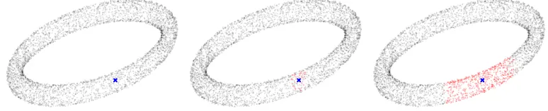
The parameter 1/ can be seen as a resolution level that determines at which distance we distinguish between design points. This parameter plays a crucial role in our approach as is explained in this section. In Figure 1 we exemplify the effect of the size of. We sampled points uniformly at random on a manifold, then added some (3-dimensional) Gaussian noise; these points are the design pointsX and are embedded on a 3-dimensional space. We then took one of the design points, and coloured red all points that fall within a given Euclidean distance of the selected design point; the three plots correspond to different choices of.
Ifis so small that no red dots would be present, then the detected dimension is 0. Ifis large enough to capture just a few nearest neighbours (leftmost plot), then we capture only the effect of the noise – 3-dimensional in our case – but arbitrary in general. Increasing
Figure 1: Design points sampled uniformly on a torus, with noise. Design points within an distance (increasing from left to right) of a fixed design point are coloured red.
(1-dimensional) surface of a tube. In either case, with much larger choices for we would capture all design points and the volume of the intersection would vanish with respect to; this would again lead the trivial case where dimension 0 is detected.
Of course the dimension can also be fractal, and we could also be interested in the dimension of just a region of the manifold in which case the choice of (and the design point that defines the neighbourhood) plays an important role again. The bottom line is that should be considered a parameter of the model (as opposed to a parameter of the estimator) in that the target intrinsic dimension should be seen as a function of ; cf. (Burges, 2010) for a similar discussion. In other words, the resolution level should be chosen in line with the goals of the analysis; to learn the structure of the noise one would pick relatively small values of, while to learn the dimension of the manifold we would have to pick larger values. This is related to the scale of the observations, and it should be taken into consideration when choosing . Another issue is that one should also account for the sample size in the form of a finite sample correction. We return to this point in Section 7 where we use some numerical experiments to illustrate this point.
Next we define and give the intuition for our estimator of the intrinsic dimension d.
4. Estimation of the Intrinsic Dimension
We start by providing some heuristic motivation for our estimator of d. Consider, for
x∈Rm,m∈
Nthe ballsV(x, m) ={y∈Rm:r(x, y)≤} for a homogeneous,
translation-invariant metricr, and denote V(m) = V(0, m). Assume, without loss of generality, that
0 ∈ X ⊆ RD, where X is an appropriate high probability set in the support of F. If is
small (or if → 0) and if F admits a continuous density f with respect to the Lebesgue measure µ, then we expect
p(x)≈
Z
X
1V(x,D)(y)f(y)dµ(y)≈f(x)·
Z
X
1V(D)(y)dµ(y),f(x)·v.
The assumption that the intrinsic dimension of the data set is d, corresponds to assuming, with mild abuse of the notation, that (for all appropriately small )
v ,µ{V(D)∩ X } ≈µ{V(d)}.
should not be sensitive to the dimension D of the data points, but instead to the intrinsic dimensiondof the data set and an -scale.
Since p,1 =E{p(X)}, we can approximate
p,1 ≈Ef(X)·µ{V(d)}.
One can estimate d by replacing p,1 by an estimator and inverting the relation above. However, this would only be feasible with knowledge of the distributionF via the constant
Ef(X) and of the parameter , which in general we do not have access to.
Arguably, the most reasonable way to get rid of the dependence onF andis to examine the data at two different scales simultaneously. For appropriately small,
p2,1
p,1
≈ µ{V2(d)}
µ{V(d)}· (6)
This is a natural idea. Looking back at Figure 1, the (hyper-)volume of the intersections (which can be inferred from the number of points in the intersection) does not give us any information about dimension; it is how this quantity scales withthat is informative.
With this approximation in mind, we define an estimator ford: for an arbitrary function
g(d) – ideallyp2,1/p,1, but in general any reasonable approximation ofµ{V2(d)}/µ{V(d)}
– the estimator is defined as (any) implicit solution ˆdn to the equality
ˆ
pn,2,1 ˆ
pn,,1
=g dˆn
, (7)
where ˆpn,,1 is any estimator for p,1, > 0. If d is an integer, then we can consider an estimator [ ˆdn], where [·] represents the argument rounded to the closest integer. Note that
the functiong is allowed to depend on n.
The need to look at the data at two different scales simultaneously should not be a surprise. The probability p,1 itself does not carry any information about dimension if
F is unknown; it is instead how p,1 scales as a function of that provides information about dimension. This notion of scaling is in fact connected with the notion of expansion dimension of (Karger and Ruhl, 2002).
For a given metricr one can numerically approximate the functionµ{V2(d)}/µ{V(d)}, but in analogy to the doubling property of the Lebesgue measure this function should be constant over , at least if is appropriately small. So a canonical choice (independent of
) would beg(d) = 2d, in which case one has an explicit estimator ford:
ˆ
dn=
log ˆpn,2,1−log ˆpn,,1
log 2 · (8)
This is just an example of a possible form that the estimator can take. However, it does suggest that at least for certain models one can expect to have explicit estimators fordthat do not require knowledge of ,F, orr and are therefore completely parameter-free.
knowledge of the distribution F. This follows from the trade-off between the standard deviation of the distributionF and the radius. Letσ >0, and sayA/σis associated with
design pointsX ∼F and A0 is associated with design pointsX0 ∼F(·/σ); then
A/σ,i,j =1{r(Xi,Xj)≤/σ}=1{r(σXi,σXj)≤}∼A
0
,i,j,
so that information aboutcannot be retrieved from the adjacency matrix without knowl-edge of the distribution F. However, if is known, one may try to flesh out lower order terms in the approximation above to reduce the bias of the estimates.
We can more precisely approximate the local connection probability as
p(x)≈f(x)·v+
Z
X
1V(x,D)(y) (y−x)
T∇f(x)dµ(y),
where∇f denotes the gradient of the density f, so that by taking expectation,
p,1 ≈Ef(X)·v· 1 + ∆
, ∆ =
ERX1V(X,D)(y) (y−X)
T∇f(X)dµ(y),
Ef(X)·v
·
For our canonical choiceg(d) = 2d we thus obtain the approximation
logp2,1−logp,1 log 2 ≈
logv2−logv+ log 1 + ∆2
−log 1 + ∆
log 2 ≈d+
∆2−∆
log 2 .
By the Cauchy-Schwarz inequality to the inner product (y−x)T∇f(x), we conclude that
|∆2−∆|
log 2 ≤ 3 log 2·
Ek∇f(X)k
Ef(X)
·.
Although the multiplier above is unknown, it depends only on F and is therefore fixed. Furthermore, it is reasonable to expect the multiplier to be of order d, since the gradient of the density should only be non-trivial alongd independent directions. This means that certain choices for the function g(d), like for example choices that are independent of the
scale , should result in a bias of order O(d·). We return to this discussion in Section 6 after we have specified the asymptotics of ˆdn for arbitrary g.
Remark 1 A similar reasoning to the one that was applied to p,1 above can be applied to other probabilities associated with the model, like for example p,2, to motivate alternative estimators for the intrinsic dimension. Although not reported here, we did not find any noticeable difference between the dˆn estimator defined in (7) and a p,2 based estimator.
From the discussion above, it is clear that the consistency of the estimators defined in (7) depends on three factors: the consistency of the estimates of p,1 that are used, the quality of the approximation in (6), and the slope of g(d) around the underlying intrinsic
5. Estimates of the Connection Probability and their Asymptotics
An estimator for p,1 is obtained by averaging off-diagonal entries of the matrix A. For
any mn≤n(mnis for now left unspecified, and is a parameter of the estimator),
ˆ
pn,,1= 1
mn
mn
X
i=1
B,i
n−1 =
2
mn(n−1)
mn
X
i=1
n
X
j=i+1
A,i,j, (9)
using the symmetry ofA. SinceEB,i/(n−1) =p,1, the estimator ˆpn,,1 is unbiased. This estimator can be evaluated in O(n mn) instructions. If we set mn =n then the execution
time may be prohibitive ifn is large so the parametermn offers some flexibility. However,
as we will see below and in Sections 6 and 7, the role of the sequencemngoes beyond just
controlling the computational complexity of the estimator. In Section 7.2, in particular, we discuss what constitutes a “good” choice formn.
The following theorem provides the asymptotics for the estimator in (9).
Theorem 2 Let mn≤n and mn→ ∞ as n→ ∞. If mn=o(n), andp,2 > p2,1, then
Sn,,−1/12·
ˆ
pn,,1
p,1
−1
d
−→N(0,1), where Sn,,1 =
p,2−p2,1
mnp2,1
. (10)
Ifmn=nthen the previous display also holds if we further assume thatn(p,2−p2,1)2 → ∞. (This assumption always holds if is fixed.)
The proof of this theorem can be found in the Appendix. This result is valid irrespec-tively of the distributionF, and holds even if→0, as n→ ∞, so that p,1, p,2 →0. The differencep,2−p2,1 =E{p(X)2} − {Ep(X)}2 is the variance of the functionp. From this
we see thatp being more variable has a negative impact on the estimation ofp,1, which is not surprising. If is fixed, thenp,1 can be estimated with ratem
−1/2
n . However, if →0
the rates may be different depending on how the probabilities involved scale with , which in turn depends on the specific distribution F and the metricr at hand.
Next we give conditions under which the estimators (7) are consistent for d.
6. Consistency of Estimates for the Intrinsic Dimension
Based on the asymptotics of ˆpn,,1from the previous section, whether the procedure outlined in Section 4 delivers consistent estimates for dor not, now depends on the specific model in question and on g(d).
Theorem 3 Consider the implicit estimators (7). Assume that the conditions of Theorem 2 required for the convergence of pˆn,,1 and pˆn,2,1 with rate m−1n /2 hold. For that , d, and
mn, assume that, asn→ ∞,
p2,1=p,1·g
n
d+o(m−1n /2)
o
Assume also that the derivative (with respect tod) ofg(d)exists, is continuous and non-zero at d. If p,1·(1−p2,1) =o
n{p,2,2−p,1·p2,1}
andmn=o(n), then as n→ ∞,
Sn,−1/2·ndˆn−d
o d
−→N(0,1), where Sn, =
∂logg(d)
∂d
2
· V
mn
where for p1,2,2 =P{r(X, Z)≤1, r(Y, Z)≤2},
V=
p2,1·p2,2−2·p,2,2·p,1·p2,1+p22,1·p,2
p2
,1·p22,1
Remark 4 In Theorem 3 we consider the case mn=o(n), which is the most relevant case in practice. The general expression forV (meaning for any sequencemn≤n) can be found in (16), in the Appendix.
Remark 5 Condition (B) controls the asymptotic bias of the estimator for d. Note that this condition should be interpreted as a condition ong and on the sequence mn, and not a condition on , since is a modelling parameter set by the user. If condition (B) does not hold, then the statement of the previous theorem is still valid if we centre dˆn with E( ˆdn) instead of d, but in that case the estimator might be asymptotically biased. Alternatively, if (B) holds with rn=o(mn), instead of mn, then we conclude thatr
−1/2
n dˆn−d
=oP(1). (Note that the condition becomes more restrictive for faster rates.)
For the explicit estimator in (8) theg(d)-dependent scaling in the variance is log(2)−2.
In this case, the bias condition (B) reduces to
p2,1 =p,1·2d+o m
−1/2
n
.
This requires the connection probabilityp,1 to approximately have a doubling property: if the distance at which vertices connect doubles, then the probability of connection goes up by a factor 2d, approximately. (Note that alsoshould in general depend onn, but we return to this point in Section 7.1.) How much leverage we have in terms of the approximation depends mostly on the sequencemnand is, in a sense, the price to pay for the computational
speed-up. However, the choice ofmn goes well beyond this.
Remark 6 Since our estimator for d only requires access tomn rows of A and A2, one can obtain several (correlated) estimates dˆ(1)n , dˆ(2)n , . . . , of d based on disjoint sets of rows if mn=o(n). From these one can estimate the variance of dˆn.
Say that we consider the following estimator for the variance
ˆ
σ2n=Vddˆ
n=
1
tn−1
tn−1
X
i=1
n
ˆ
d(ni)−d¯n
o2
, with d¯n=
1
tn tn
X
i=1 ˆ
d(ni),
where tn∈Nis at most n/mn. It is straightforward to check that
Eσˆn2 =σ2
h
1−ρdˆ(1)n ,dˆ(2)n i
where ρ(X, Y) represents the correlation between X and Y. Making use of the fact that
ˆ
pn,,(i) 1 and pˆn,(i)2,1 are independent for i∈N, we have
Vdˆ(1)n ,dˆ(2)n =
1
log(2)2
h
Vlog ˆp(1)n,,1,log ˆp (2)
n,,1 +V
log ˆp(1)n,2,1,log ˆp(2)n,2,1 i
.
Using the approximation3 V(logX,logY) ≈ V(X, Y)/(EX·EY), it is enough to look at Vpˆ(1)n,,1,pˆ
(2)
n,,1 . If we denote the range of rows associated with these two estimators as respectively I1 andI2, then writing the covariance as a four-fold sum, we get
Vpˆ(1)n,,1,pˆ (2)
n,,1 =
2
mn(n−1)
2
X
i1∈I1
X
i2∈I2 n
X
j1=i1+1
n
X
j2=i2+1
V A,i1,j1, A,i2,j2
≤ 4
n−1 p,2−p
2
,1
,
where we use the fact that since I1∩I2=∅, then V A,i1,j1, A,i2,j2
=p,2−p2,1 ifj1 =j2, and V A,i1,j1, A,i2,j2
= 0, if j1 6=j2. Finally, under the conditions of Theorems 2 and 3, we can put everything together to bound
Eσˆ2n−σ2
.
mn
n ·
Sn,,1
Sn,
;
this upper bound converges to zero for appropriate , if mn=o(n).
Note that when the metric r is induced by the Euclidean normk · k2, andmn=n, the
estimator ˆpn,,1 (as a function of ) coincides with a realisation of the so-called correlation integral; cf. (Camastra and Vinciarelli, 2002). This is defined in the following way. With
x1, . . . , xn denoting points on a manifold whose dimension we would like to measure, let
Cn() =
2
n(n−1)
n−1
X
i=1
n
X
j=i+1
1{kxi−xjk2≤}; (11)
the correlation integral C() is the limit, when n → ∞, of Cn(). The underlying idea
behind the intrinsic dimension being dis that C() should scale liked so that the limit as
→0 of log{C()}/log() isd; this is then called the correlation dimension, which is a type of fractal dimension. Following up on Remark 1, basing our estimator on p,2 would lead to a variation on the correlation integral above. We found no advantage in using the p,2 based estimator over the p,1 based one.
Some estimators for intrinsic dimension like that of (Grassberger and Procaccia, 1983) are based on the idea of regressing log{Cn()} on log(), and estimating the (correlation)
dimension from the slope of the fit. However, based on the discussion from Section 3, this slope actually corresponds to some average dimension over different scales, which is not what we are interested in; cf. Fig. 3.3 of Lee and Verleysen, 2007, for an example of the scale dependence of the correlation integral. Further, this also makes extensive use of
distances between the observations, while we rely only on the neighbourhood information provided by adjacency matrices.
As we argue in the previous section, one has to examine the data at (at least) two different scales to derive meaningful information about dimension, and this has been noted in the literature before. (K´egl, 2002) proposed a scale dependent notion of correlation dimension based on
Dn(1, 2) =
log{Cn(2)} −log{Cn(1)} log(2)−log(1)
(12)
This improves upon the idea of regressing the logarithms of the empirical version of the cor-relation integral (cf. Grassberger and Procaccia, 1983; Pettis et al., 1979) on the logarithm of by allowing one to focus on a specific range of scales. Indeed, this is closely reflected in our estimator ˆdn, although we distinguish ourselves from other approaches by deriving
the asymptotic distribution of our estimator within a flexible framework; to the best of our knowledge the central limit theorem that we derive is new to the literature.
Other approaches to intrinsic dimension estimation follow similar ideas but make use of other notions of dimension like for example Hausdorff dimension, information dimension, box counting dimension, (generalised) expansion dimension, packing dimension, and also local versions of these concepts. The success of such approaches depends mostly on how computationally tractable computing the estimate of the dimension is, and how adequate the particular notion of dimension at hand is for the model under consideration.
Another approach corresponds to the maximum likelihood estimator of (Bickel and Levina, 2004). This estimator is based on maximising the likelihood obtained by assuming that the observations come from a homogeneous Poisson process. The estimator is then based on distances to the k-the nearest neighbour of each point, with k interpreted as a “bandwidth” parameter of the estimator. Another estimator based onk-nearest-neighbours is that of (Kleindessner and von Luxburg, 2015). In both cases the connection between k
and the scale at which we estimate dimension has not yet been explored in detail, however. The disadvantage ofk-nearest-neighbour approaches seems to be that the way in which the distance of an observation to its k nearest neighbour scales with dimensions may heavily depend on the underlying distribution of the data. Although this does open the door to sharper estimates of the intrinsic dimension, this is done at the expense of needing more information about the distribution of the data. Besides this, relatingkto the scale at which the intrinsic dimensions is being estimated also seems to be difficult.
The approaches mentioned above, as well as our approach, are examples of so called geometric methods. A different class of methods are eigenvalue (or projection) methods. These stem from the work of (Fukunaga and Olsen, 1971); see also (Bruske and Sommer, 1998). These methods are typically based on principal component analysis (PCA) and estimate the dimension based on how many eigenvalues are above certain (small) threshold. They seem to be less useful for estimating intrinsic dimension because of the difficulty of determining what constitutes an appropriate threshold; cf. (Verveer and Duin, 1995).
● ● ● ● ● ● ● ● ● ●
ε =2
d
lo
g
{
mn Sn,
ε
}
1 2 3 4 5 6 7 8 9 10
−12 −10 −8 −6 −4 −2 0 2
4 ● Uniform
Gaussian Cauchy Exponential Beta ● ● ● ● ● ● ● ● ● ●
ε =1
d
lo
g
{
mn Sn,
ε
}
1 2 3 4 5 6 7 8 9 10
−12 −10 −8 −6 −4 −2 0 2 4 ● ● ● ● ● ● ● ● ● ●
ε =1 2
d
lo
g
{
mn Sn,
ε
}
1 2 3 4 5 6 7 8 9 10
−12 −10 −8 −6 −4 −2 0 2 4
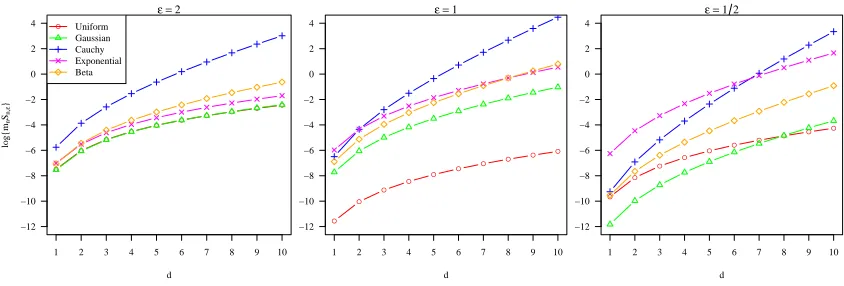
Figure 2: Effect of the distribution of the design points, d, and on the logarithm of the asymptotic variance of our estimator ford. The three plots correspond to∈ {2,1,1/2}, left to right. In each plot, each line corresponds to a different distribution for the design points.
7. Numerical Results
In this section we present some numerical results. We start by exemplifying in Section 7.1 how the probabilities p,1 and p,2 determine the bias and variance of our estimator for different distributions for the observationsX. Section 7.2 is about the consequences of the choice of the sequencemnin our estimator. In Section 7.3 the performance of our estimator
is evaluated for different combinations of dimension d and resolution 1/. The main goal of these first three subsections is to understand what constitutes a good choice for the sequencemn that features in the definition (9). Section 7.4 concerns a non-trivial choice for
the function g (meaning a choice other than 2d), as well as other types of bias correction.
In Section 7.5 we illustrate the effect of noise on our estimator. Finally, in Section 7.6, we apply our estimator to a batch of data sets of both simulated, and real data. To simplify the exposition, in all cases the metricr is the Euclidean distance.
7.1 Scaling of p,1 and p,2, and their Influence on the Bias and Variance of dˆn
The probabilities p,1 and p,2 play an important role in our approach. The quantity
{p,2 −p2,1}/p2,1 is the variance of the function p(x)/p,1, which is the relative connec-tion probability at each site x. We see, for example, that if mn = o(n), then the scaling
mn·Sn, that features in the asymptotics for our estimator fordis up to a constant factor
the variance ofp(X)/p,1−p2(X)/p2,1. However, this quantity still depends on and d, so it is interesting to see how it behaves for different distributions for the design points.
In Figure 2 we plot the logarithm ofmn·Sn,, as a function of the intrinsic dimensiond
for several different choices for the distribution of the design points, for three choices of . Ifis fixed, thenmnSn, is just the constant that features in the rate of convergence of the
estimator of ˆdn. (The curves were computed by numerical integration, but are otherwise
exact.) The coordinates of the design points Xi were sampled independently from the
ε =2
d
lo
g
{
p2ε,1
pε,1
}
log
(
2
)
1 2 3 4 5 6 7 8 9 10
1 2 3 4 5 6 7 8 9 10 ● ● ● ● ● ● ● ● ● ● ● Uniform Gaussian Cauchy Exponential Beta
ε =1
d
lo
g
{
p2ε,1
pε,1
}
log
(
2
)
1 2 3 4 5 6 7 8 9 10
1 2 3 4 5 6 7 8 9 10 ● ● ● ● ● ● ● ● ● ●
ε =1 2
d
lo
g
{
p2ε,1
pε,1
}
log
(
2
)
1 2 3 4 5 6 7 8 9 10
1 2 3 4 5 6 7 8 9 10 ● ● ● ● ● ● ● ● ● ●
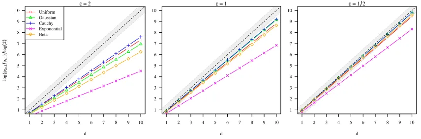
Figure 3: Effect of the distribution of the design points,d, andon{logp2,1−logp,1}/log(2). Left to
right, the plots correspond to∈ {2,1,1/2}. The shaded area corresponds tod±1/2.
large d (about d ≥ 5) the lines increase roughly linearly, which would mean that the constants in the asymptotic statement in Theorem 3 increase exponentially with d. In general,dis fixed, but these plots give an indication that if the intrinsic dimension is large, then in order to attain a given level of precision, one should need a fairly large number of observations. This should give a notion of when the asymptotics described in Section 6kick in. The effect of , on the other hand, does not seem too pronounced and affects mostly how the lines behave when the intrinsic dimension dis relatively small.
While the variance of the estimator is, up to the scaling {∂logg(d)/∂d}2, only model
dependent, the bias depends greatly on the functiongused in the definition of the estimator.
In particular it depends on how wellg(d) approximatesp2,1/p,1 as prescribed by the bias condition (B). As discussed in Section 4, for appropriately small , it should hold that
p2,1/p,1 ≈2d, making g(d) = 2d our canonical choice for g. For this choice of g and for
the same distributions as before, in Figure 3 we plot d7→ {logp2,1 −logp,1}/log(2), for different ; we compare it with the identity d7→d.
In the plots above, the black dotted line along the diagonal is the identity, and the grey shaded area encompassesd±1/2 (for reference). As before, the remaining lines correspond to different distributions for the design points. As expected from the discussion in Section 4, as gets smaller, these lines mimic the doubling property of the Lebesgue measure more closely so that d 7→ p2,1/p,1 indeed gets closer to d 7→ 2d. The plots also suggest that considering g(d) = 2d should lead to the dimension being systematically underestimated,
and that one may want to consider a multiplicative correction based on . In a sense, this is the price to be paid for having a parameter-free estimator.
Part of the bias is a consequence of the fact that, in general, we do not have access to a good (model dependent) function g. For example, if g is constant over , as discussed in Section 4, the bias should, in fact, be of order . One should therefore consider to take
As it turns out, there is a justification for taking=nconverging to zero. The rationale
is the following. Typically, there will be noise in our data so that the support of F is an enlarged version of the manifold whose dimension we would like to estimate. If the design points are relatively concentrated, in the sense that Pr(0, X) > x . exp(−x2), x > 0,
say, then, by the union bound,
P
n
max
i=1,...,nr(0, Xi)>
p
δlogn
o ≤
n
X
i=1
P
n
r(0, Xi)>
p
δlogn
o
.n1−δ, δ >1.
In other words, if1 is to express the distance at which we would like to analyse the data, then if we observe onlynpoints and take≡1, we are overestimating the typical distances between points by roughly a factor√logn. In a sense, this growing spread can be thought of as arising from noise, so that we should therefore establish connections at a slightly smaller distance, say for instance n = 1/
p
log(1 +n), 1 > 0. This can also be seen as a finite sample correction for the estimator; cf. (Grassberger, 1988). Another reason to consider
of this kind would be to ensure that the adjacency matrices that we work with remain relatively sparse. This means that we avoid storage problems even when the sample sizen
is large. This can also be motivated from the point of view of discriminability; cf. (Beyer et al., 1999; Weber et al., 1998; Houle, 2013). If the dimensionality of the data is high, then distance values are less discriminative, in the sense that they tend to concentrate more around the mean of their distribution. Because of this, it makes sense to increase the strictness with which new connections are accepted as the sample size grows.
This has three important consequences. The first is that for the parameter-free es-timator (8), with the finite sample correction described above should have squared bias
O(1/logn). This means that the sequence mn should be set to O(logn) to balance
vari-ance and squared bias. The proverbial less is more comes to mind: pickingmn large and
averaging over many vertices leads to deceptive results, since the variance of the estimate is reduced, while the bias remains unchanged. This is an inherent feature of estimators obtained via inversion, but it is something that is invariably missed in the literature – es-timates are strongly concentrated around biased eses-timates. This is undesirable from the point of view of uncertainty quantification; see also the next section. By doing this our estimator attains the minimax rate for this problem which is known to be logarithmic; cf. (Koltchinskii, 2000).
The second consequence follows from the first: setting mn = O(logn) leads to an
algorithm with complexity O(nlogn). This is a great advantage over competing algo-rithms whose execution time typically scales likeO(n2), sometimes like O(D n2); cf. Table 1 in (Eriksson and Crovella, 2012). Finally, sincemn is rather small compared withn, this
means that we are estimating dbased on the degrees of only a few vertices. By repeating the estimation for disjoint sets of vertices we can estimate the standard deviation of the estimator without a need for resampling. The conclusion is that picking smallmnis better,
both from a theoretical and practical perspective.
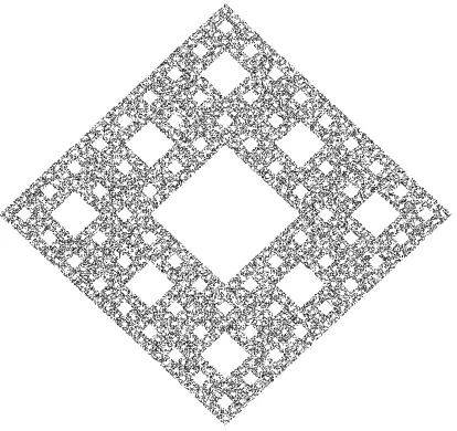
Figure 4: Example of 5·104 points sampled uniformly at random on a Sierpinski carpet. Points like these are used as design points in the simulations in this section.
7.2 Different Choices of mn
In this section we look more closely at the choice ofmn by exemplifying the effect that the
choice of this sequences has on: a) the bias, b) the variance, and c) the execution time. To have a nontrivial dimension we consider design points sampled uniformly at random on a Sierpinski carpet. This can be done in the following way. Consider
P0 =
0 0
, and C =
0 1/2 1 1/2 0 −1/2 −1 −1/2 1 1/2 0 −1/2 −1 −1/2 0 1/2
.
Let ei = [0 · · · 0 1 0· · · 0]T, i= 1, . . . ,8, be unit vectors that have a 1 in the i-th position,
and let ij ∼ U{1, . . . ,8}, j = 1,2, . . ., be a sequences of independent, discrete uniform
random variables taking values on {1, . . . ,8}. A point can be drawn uniformly at random on a Sierpinski carpet as
P =P0+C
∞
X
j=1
3−j·eij.
Figure 4 depicts 5·104points drawn according to this procedure. In practice we truncate the sum at 100 terms. (Note that this is accurate enough to get the neighbourhood matricesA
exactly.) The correlation dimension of the Sierpinski carpet is, to the best of our knowledge, unknown, but its Hausdorff dimension is log 8/log 3 ≈ 1.89, which should provide a good indication to what the intrinsic dimension should be.
In this section we ran our algorithm for all combinations ofn= 10·2γ,γ∈ {0,1, . . . ,8}, and mn either log(n) or nγ, γ ∈ {1/4,1/2,3/4,1}. The parameter was set to n =
mn
log(n) n1/4 n1/2 n3/4 n
n
10 1.1780 (0.78) 1.1243 (0.55) 1.0945 (0.39) 1.0877 (0.32) 1.0861 (0.26)
20 1.2678 (0.54) 1.2528 (0.43) 1.2483 (0.33) 1.2409 (0.24) 1.2367 (0.18)
30 1.3784 (0.49) 1.3718 (0.40) 1.3673 (0.26) 1.3631 (0.17) 1.3602 (0.12)
40 1.4852 (0.44) 1.4781 (0.35) 1.4668 (0.20) 1.4660 (0.12) 1.4636 (0.08)
160 1.5491 (0.32) 1.5441 (0.27) 1.5434 (0.15) 1.5398 (0.08) 1.5395 (0.05)
320 1.6037 (0.28) 1.5963 (0.22) 1.5925 (0.12) 1.5930 (0.06) 1.5923 (0.03)
640 1.6395 (0.27) 1.6376 (0.19) 1.6332 (0.09) 1.6320 (0.04) 1.6320 (0.02)
1280 1.6595 (0.22) 1.6622 (0.18) 1.6596 (0.07) 1.6595 (0.03) 1.6597 (0.01)
2560 1.6790 (0.22) 1.6770 (0.15) 1.6778 (0.06) 1.6768 (0.02) 1.6772 (0.01)
Table 1: Results for the estimation of the intrinsic dimensiondfor random Sierpinski carpet design points, for different combinations ofn andmn. For each combination, ˆdn was estimated 105 times; we
display the mean estimate, and in parenthesis the standard deviation among the estimates.
was used here to ensure that is on the right scale. These simulations were repeated 105 times and the results are averaged.
Table 1 summarises the average and standard deviation of the estimates that were obtained for each combination of n and mn. Irrespectively of the sequence mn, it is clear
that as ngrows the estimates stabilise. This is in tune with our consistency result, also in that the reduction of the bias is rather slow. It is also clear from the results that the sequence
mn does not seem to have much influence on the quality of the estimate, particularly as n
grows. This is also in tune with our results: larger mn does increase the precision of the
estimates of the probabilities p,1; what mainly determines the precision of the estimate of dis the bias introduced by the function g, though. The effect of mn on the standard
deviation is also as expected: increasing eithernormngenerally leads to a decreased of the
variability of the estimate. From this it might seem reasonable to set mn to a large value
(after all, it does reduce the variance of the estimator without reducing precision). There are however two good reasons to keep the growth of mn slow.
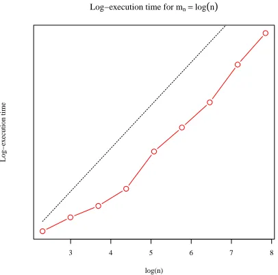
The first reason is execution time. Figure 5 shows the evolution of the average execution time of the algorithm as a function ofn, whenmn= log(n). For comparison, Table 2 shows
the average execution time as a multiplier of the execution time for mn = log(n), for the
same value ofn. In words: the numbers on the table indicate how much slower it is to set
mn to each choice, compared to just setting it to log(n).
The conclusion from Figure 5 is that the execution time for mn= log(n) grows roughly
linearly with n. On the other hand, from Table 2, for other choices of mn the execution
time quickly becomes prohibitive, particularly for faster-growing sequences mn.
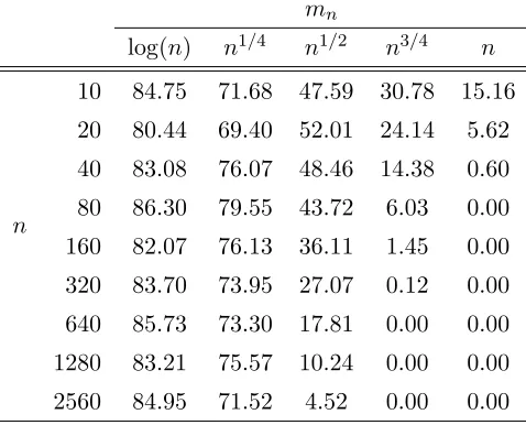
There is a second reason to set mn = O{log(n)}. Table 3 shows the percentage of
runs in which dfalls within 2 standard deviations from ˆdn. The effect of mn is clear. The
3 4 5 6 7 8
Log−execution time for mn=log(n)
log(n)
Log−e
x
ecution time
Figure 5: The evolution of the average execution time of our algorithm as a function ofn when mn =
log(n). The plot is on a log-log scale. For reference, the dashed line represents log(n) plotted against log(n)−10. The execution time grows roughly linearly withn.
mn
n1/4 n1/2 n3/4 n
n
10 1.13 1.65 2.14 3.20
20 1.29 1.63 2.94 5.98
40 1.34 2.63 5.59 12.72
80 1.31 3.51 9.75 28.43
160 1.20 3.57 12.10 42.46
320 1.52 5.24 21.72 90.87
640 1.91 8.05 39.19 194.22
1280 1.53 9.03 53.86 325.12
2560 1.99 12.68 89.80 638.54
Table 2: Average execution times for the algorithm. For each combination of n and sequence mn, the
respective entry in the table specifies how many times larger the execution time of the algorithm is compared to using mn = log(n). For example, if we setmn =n, then, whenn is 2560, we
have to wait more than 638 times longer for the algorithm to terminate than if we had used
mn= log(n).
Since the estimates are biased, if the sequence mn grows too quickly, then the variance
mn
log(n) n1/4 n1/2 n3/4 n
n
10 84.75 71.68 47.59 30.78 15.16
20 80.44 69.40 52.01 24.14 5.62
40 83.08 76.07 48.46 14.38 0.60
80 86.30 79.55 43.72 6.03 0.00
160 82.07 76.13 36.11 1.45 0.00
320 83.70 73.95 27.07 0.12 0.00
640 85.73 73.30 17.81 0.00 0.00
1280 83.21 75.57 10.24 0.00 0.00
2560 84.95 71.52 4.52 0.00 0.00
Table 3: Percentage of the 105 runs where the true value ofdis within 2 standard deviations of ˆdn.
biased mean. In effect, because the bias and the variance are out of balance, the standard deviation fails to properly quantify the uncertainty in the estimate. Also remember that if
mn is small, then we can produce several estimates of d, from which we can estimate the
standard deviation without a need for resampling.
To conclude, the sequence mn affects the variance of the estimator ˆdn, but it does not
affect the bias of the estimate, which comes mostly from the functiong. Faster growingmn
therefore leads to estimates that are overly concentrated around their (biased) mean, so that their variability gives misleading information about the uncertainty in the estimate. Such choices ofmnalso lead to a large computations cost. Therefore, settingmn=O{log(n)}is
arguably the correct choice to make.
7.3 Different Combinations of dand n
In this section we show how the estimator ˆdn behaves for different combinations of d and
n. We set the distribution of the design pointsX ∼Nd(0,I), for d∈ {1,2,3,4,5,10}, and
chose n ∈ {103,104,105,106,107}; irrespectively of the dimension we always set =n =
4/(logn)1/2. Based on the discussion from the previous section, the parametermn was set
to max(1,logn).
Table 4 below contains the results of estimating the intrinsic dimensiond10 times: for each combination of n and d we sampled an adjacency matrix, estimated d10 times from 10 disjoint subsets of mn vertices (chosen at random, without replacement); the average
and (in brackets) the standard deviation of the 10 estimates make up the entries of the table. Note that since we only average over a relatively small number of vertices in the graph, producing Table 4 does not actually require any resampling; the same data set can be used (for each combination of nand d). Note also that for the choice of mn above, the
n
103 104 105 106 107
d
1 0.49 (0.15) 0.58 (0.11) 0.54 (0.12) 0.63 (0.07) 0.71 (0.15)
2 0.91 (0.18) 1.18 (0.19) 1.31 (0.26) 1.41 (0.25) 1.53 (0.17)
3 1.76 (0.24) 1.99 (0.29) 2.23 (0.36) 2.28 (0.34) 2.51 (0.20)
4 2.55 (0.50) 2.94 (0.30) 3.23 (0.42) 3.05 (0.44) 3.42 (0.32)
5 3.24 (0.37) 3.61 (0.38) 3.96 (0.43) 4.31 (0.18) 4.39 (0.44)
10 5.95 (0.61) 7.46 (0.53) 8.59 (0.70) 8.81 (0.70) 8.97 (0.75)
Table 4: Results for the estimation ofd for Gaussian design points for different combinations of d and
n. For each combination ˆdn was estimated 10 times; we display the mean estimate, and in
parentheses the standard deviation among the estimates.
A few things are clear from the results in Table 4. As hinted in Section 7.1, the estima-tor tends to underestimate the true intrinsic dimension, especially if the dimension is large. However, as far as recuperating the integer dimension, the estimator performs well, espe-cially considering that the data is entirely comprised of random fluctuations. The standard deviation also does a good job at quantifying the precision of the estimate.
We emphasise that the estimates are parameter free – one can improve the results with extra knowledge about the distribution of the data. We do this in the following subsection.
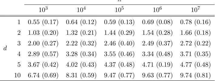
7.4 Non-canonical Choice of g(d), and Bias Corrections
In this section we propose some modifications of our estimator aimed at removing (or at least mitigating) its bias. Since we know that the estimator ˆdn systematically underestimatesd,
a simple way of obtaining a “bias corrected” estimator is by scaling ˆdn up. We consider
three different ways of doing this.
Following the discussion at the end of Section 4, where we justified that the bias should be of order O(d·), we consider
˜
dn= ˆdn·
1 + 2 log(2)·
· (13)
n
103 104 105 106 107
d
1 0.55 (0.17) 0.64 (0.12) 0.59 (0.13) 0.69 (0.08) 0.78 (0.16)
2 1.03 (0.20) 1.32 (0.21) 1.44 (0.29) 1.54 (0.28) 1.66 (0.18)
3 2.00 (0.27) 2.22 (0.32) 2.46 (0.40) 2.49 (0.37) 2.72 (0.22)
4 2.89 (0.57) 3.28 (0.34) 3.55 (0.46) 3.34 (0.48) 3.71 (0.35)
5 3.67 (0.42) 4.02 (0.43) 4.37 (0.48) 4.71 (0.19) 4.77 (0.48)
10 6.74 (0.69) 8.31 (0.59) 9.47 (0.77) 9.63 (0.77) 9.74 (0.81)
Table 5: This table contains the results of repeating the experiment from the previous section, but we compensate for the bias by considering a multiplicative correction.
Comparing these results with those of Table 4, we see that indeed this correction seems to substantially improve the estimates.
One can also consider other choices for the function g to reduce the bias. The idea is
to use knowledge of the distribution of the design points to select a better suited candidate for this function. This also leads to more precise estimates of the intrinsic dimension. If
X ∼ Nd(0,I), independent of Y ∼ Nd(0,I) then Z = X−Y ∼ Nd(0,2I), so that, if we
abbreviate Z ={z∈Rd:kzk ≤}, then
p,1 =P(kX−Yk ≤) =P(kZk ≤) = 1
(4π)d/2
Z
Z
e−14kzk 2
dz= v
(4π)d/2
Z 1
0
e−14u 22
du,
wherev represents the volume of ad-dimensional Euclidean ball of radius. The integral
above can be expressed in terms of the Gauss error function erf, so that
p,1= (4π)−d/2·v·
√ π
·erf(/2), whence
p2,1
p,1
= 2d·erf()/2
erf(/2)·
What is arguably the ideal choice for the functiong is then
g(d) = 2d·
erf()/2
erf(/2), leading to ¯
dn= ˆdn+
log{erf(/2)} −log{erf()/2}
log 2 ,
where ˆdn is the canonical estimator from (8). Note that using the exact function g(d)
does not entirely remove the bias of the estimate since g(d) is not linear in d, and since
ˆ
pn,2,1/pˆn,,1 is not an unbiased estimator forp2,1/p,1. Note also that the correction factor depends only on, but not ond. To understand the effect of this new estimator based on the more precise choice ofg(d), we repeat the numerical experiment of the previous section now
for the estimator ¯dnfrom the previous display; Table 6 summarises these results. Comparing
Tables 4 and 6, it is clear that, as one would expect, a more informed choice for mappingg
n
103 104 105 106 107
d
1 1.04 (0.25) 1.04 (0.11) 1.06 (0.14) 1.00 (0.11) 0.99 (0.15)
2 1.63 (0.22) 1.76 (0.33) 1.69 (0.24) 1.80 (0.27) 1.84 (0.17)
3 2.42 (0.37) 2.45 (0.48) 2.54 (0.23) 2.48 (0.33) 2.73 (0.33)
4 2.99 (0.41) 3.23 (0.35) 3.71 (0.38) 3.64 (0.32) 3.50 (0.28)
5 3.98 (0.54) 4.37 (0.47) 4.49 (0.44) 4.36 (0.34) 4.30 (0.33)
10 6.56 (0.67) 7.87 (0.60) 8.47 (0.79) 9.63 (0.82) 9.39 (0.71)
Table 6: This table contains the results of repeating the experiment from the previous section, but instead using the true underlying functiong(d) that mapsdto the ratiosp2,1/p,1.
n
103 104 105 106 107
d
1 0.79 0.80 0.78 0.77 1.01
2 1.27 1.56 1.83 1.91 1.87
3 2.24 2.57 2.95 2.96 2.91
4 3.55 3.54 4.07 3.93 4.06
5 3.98 4.37 4.82 4.67 5.27
10 7.17 8.52 9.99 10.21 10.47
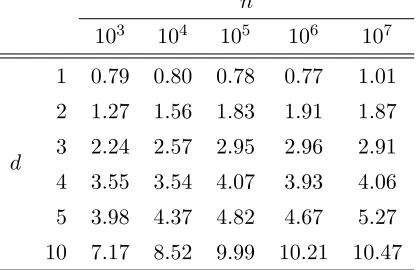
Table 7: This table contains the results of repeating the experiment from the previous section, but we compensate for the bias by adding two standard deviations to the estimate.
seems to be small. This is most likely due to the fact that the multiplicative correction is better at compensating for the bias induced by the bias of our moment estimator of
p2,1/p,1.
As a third and final alternative, one can also shift the estimates up by a factor depending on the standard deviations of the estimates. This is motivated by the fact that our choice of mn =O{log(n)} balances squared bias and variance. (Again, the standard deviation is
estimated using the same data as ˆdn without any need from resampling.) Table 7 presents
the results of adding (since we otherwise under-estimate) two standard deviations to the corresponding estimate ˆdn.
This correction performs well, particularly considering that it requires no extra infor-mation about the distribution of the data. Overall this seems to present the best correction for exactly this reason.
1 2 3 4 5
1
2
3
4
5
n = 10^3
s
d
^n ●
● ● ● ●
1 2 3 4 5
1
2
3
4
5
n = 10^4
s
d
^
● ●
● ●
●
1 2 3 4 5
1
2
3
4
5
n = 10^5
s
d
^
● ●
●
● ●
● SNR = 1 SNR = 2 SNR = 4 SNR = 8 SNR = 16 SNR = 32 SNR = 64
Figure 6: The estimator’s sensitivity to noise. Each plot corresponds to a different sample size, from left to right:n∈ {103,104,105}. The lines correspond to different estimates of the intrinsic dimension for different values ofs, and the different colours correspond to different SNR.
correction still improves the canonical estimate ˆdn considerably. However, this does not
change the fact that one will always need a large sample sizenwhen the intrinsic dimension
dis large.
7.5 Effect of the Noise
An important aspect to be taken into consideration is the robustness of the estimation procedure to the presence of noise. Irrespectively of the nature of the observations, if they are corrupted with enough noise, the estimation procedure will only detect the noise. In this respect we would like to see how sensitive the estimator is to the presence of noise. To see if this, we sampled design pointsX(s) inR5 according to
Xi(s)i.i.d.∼ N5
n
0,diag
s
z }| {
σsignal2 , . .
5−s
z }| {
., σnoise2 o
, i= 1, . . . , n, s= 1, . . . ,5.
We set = n = σsignal(2 logn)−1/2, and ran our estimation procedure on the adjacency matrix obtained fromX(s) fors= 1, . . . ,5. Each plot in Figure 6 corresponds to a different sample sizen∈ {103,104,105}. The coloured lines in each plot correspond to the 5 estimates
ˆ
dn, averaged over 10 disjoint sets of vertices. Different colours correspond to different signal
to noise ratio (SNR); namely, we fixed σsignal = 1 and chose σnoise such that SNR =
σsignal2 /σnoise2 ∈ {1,2,4,8,16,32,64}.
The estimator performs as intended. Consider first the rightmost plot in Figure 6, where
n d D Data set d˜n
1 1000 1 3 Uniform on a helix 1.25 (0.16)
2 1000 2 3 Swiss roll 2.44 (0.59)
3 1000 5 5 Independent Gaussian 5.26 (1.15)
4 1000 7 8 Uniform on a sphere 6.66 (0.16)
5 5000 7 8 Uniform on a sphere 7.10 (0.08)
6 1000 12 12 Uniform on [0,1]12 8.70 (0.61) 7 5000 12 12 Uniform on [0,1]12 9.65 (0.35) 8 698 – 64×64 Isomap faces 4.22 (0.70)
9 481 – 512×480 Hands 2.14 (0.35)
10 7141 – 28×28 MNIST “3” 15.62 (0.11)
11 6824 – 28×28 MNIST “4” 15.65 (0.16)
12 6313 – 28×28 MNIST “5” 15.45 (0.07)
Table 8: Numerical experiments from Section 4.2 of (Kleindessner and von Luxburg, 2015) for different simulated and real data sets. For each data set we indicate the sample size, intrinsic dimension
d, and ambient dimensionD. The first seven data sets are simulated, while the last five are real. The intrinsic dimension of the real data sets is unknown.
that the mass of the distribution is concentrating on a lower dimensional subspace, and gradually changing to reflect this. For smaller sample sizes, as per the discussion from Section 7.1, the rightmost points in the plot are not reliable estimates.
7.6 Comparison with Other Estimators
We compare our estimator with competing approaches from the literature. To do this we repeat the numerical simulations of Section 4.2 of (Kleindessner and von Luxburg, 2015), which is conceptually close to our estimator. Our results can then be compared directly with the results from their Table 1. Note that we base our estimates on two (symmetric) adjacency matricesA andA2, while the estimators from (Kleindessner and von Luxburg,
2015) are based on a (directed)k-nearest neighbour graph, so that both approaches require the same number of measurements. We consider twelve data sets; seven consist of simulated data, and five of real data. Table 8 contains the results.
The simulated data sets are self explanatory. The Isomap faces data set4 contains 698 images (D= 64×64 pixels) of a rendered face of a sculpture taken from different angles, under different lighting conditions. TheHandsdata set5contains 481 frames (D= 512×480 pixels) from a video of a hand holding a rice bowl and revolving it while moving from right
4.http://isomap.stanford.edu/datasets.html
to left. TheMNIST data sets6 contain 7141, 6824, and 6313 images (D= 28×28 pixels) of handwritten digits “3”, “4”, and “5”, respectively.
About the choice of for the experiments. For every synthetic data set we set = 4/(logn)1/2 as before. For the real data sets this turned out to be inappropriate since the observations are on completely different scales. We scaled up so that the resulting adjacency matricesA and A2 were neither complete graphs nor empty graphs, since this
would lead to trivial estimates. This turn out to give us equal to 14, 17, 1600, 1600, and 1600, for data sets 8–12, respectively. In practice this can be achieved based on some notion of the scale of the observations, or based on a preliminary analysis, simulated data sets, or subsamples. In all experiments we setmn= 2 logn.
Our estimator compares quite well with the competing approaches, particularly as far as recuperating the integer dimension is concerned; the results are perhaps closer to the ones obtained by the estimator of (Levina and Bickel, 2004), but contrary to their estimator we do not require any knowledge about how the distance from a given point to its k -nearest-neighbour scales, or any distance data, or for any parameters to be set in the estimator. Also, the computational complexity of our estimator scales like O(nlogn), considerably smaller than the typical O(n2). Furthermore, the results in each row of Table 8 were obtained from a single data set, without repeated sampling. Because of this we can provide standard deviations for our estimates without a need to resample the data, including for the real data sets. These standard deviations are much more realistic than the ones associated with competing approaches. We suspect that this is because for those it is difficult to properly balance the variance and the squared bias of the estimator, resulting in estimates that are overly concentrated around their biased means.
For the simulated data sets the true dimension is recuperated with good accuracy, with the exception of the sixth and seventh data set where the intrinsic dimension is relatively high. Indeed, as discussed in Section 7.1, in order to recuperate the intrinsic dimension consistently, the sample size should be quite large compared to the intrinsic dimension, since the minimax rates for the problem are logarithmic in n. This also comes from the fact that the support of the data set is rather unstructured, unlike for example data set 2, 4, and 5, or even 10, 11, and 12.
Less can be said about the results for the real data sets since the true intrinsic dimen-sion is unknown. However, our results are comparable to the ones obtained by competing approaches. In particular, in all cases the intrinsic dimension is substantially smaller than the ambient dimension. For the Isomap faces data set we estimate the intrinsic dimension as 4; although the statue is 3-dimensional, the different lighting conditions may explain the fact that we detect an extra dimension in the data set. For theHands data set we estimate the dimension as 2.14. One would probably expect the dimension to be 3, but given the symmetries in the hand and bowl, and that the images actually make up a smooth anima-tion may explain the lower estimate. As for theMNIST data set, it seems reasonable that the estimates are not too different for the three digits. Also, if one were to parametrise the digits in terms of lengths, relative angles, and curvatures of the line segments, the estimate seems rather natural.
8. Discussion
In this paper we propose a method to estimate the intrinsic dimension of high-dimensional data sets. The approach combines the notion of correlation dimension with the doubling property of the Lebesgue measure to provide a computationally tractable estimator for data sets with (potentially) scale-dependent dimension. The approach does not require any parameters to be chosen, other than the scale at which one would like to estimate the di-mension. This is particularly useful for data that live on manifolds whose dimension may be different at different scales, data sets corrupted with noise, or whenever not much is known about the distribution of the data. We compute the estimator’s asymptotic distribution and rate of convergence. The rate that we obtain matches the logarithmic minimax rate for the (easier) problem where one has access to the observations – not just whether each pair of observations is close or not – and is therefore optimal. The estimator can be quickly evaluated inO(nlogn) steps which is also an advantage over competing approaches, whose execution time typically scales likeO(n2). Also in terms of storage there are advantages be-cause the adjacency matrix that we base our estimator on will typically be sparse (since the underlying graph is embedded in a Euclidean space). Our results provide important infor-mation for algorithms commonly used to perform dimensionality reduction, learn manifolds, compress information, do statistical adaptation, and design efficient algorithms.
Distance-based estimators usually require rather (distribution specific) knowledge since one needs to know quite precisely how distances between perturbed observations scale. These also usually require certain bandwidth parameters to be defined without an auto-matic, or data driven way of picking them. Rather than assuming that we have access to the observations (or distances between them), we simply assume that we observe a graph encoding whether observations are close or not at the scale we are interested in. This is particularly relevant when dealing with large data sets. Modelling the resulting graph as a random connection model allows us to provide bounds on the probability of recuperating the correct intrinsic dimension of the data set, under a mild identifiability condition.
Our numerical experiments show that the intrinsic dimension can be well recuperated even without access to any distance information between the observations. Furthermore, our estimator properly picks up on the uncertainty of the estimate (the standard deviation of the estimator can be estimated without need for resampling), which can be used to avoid the estimator to be overly concentrated around its biased mean. Distance-based estimators tend to be much more costly, computationally. The estimator is parameter-free, but it can easily be improved by using any knowledge one may have about the distribution of the data. This is done by incorporating this knowledge into the choice of the functiong that
features in the definition of the estimator.