Consensus via Adaptive Gain Controllers Considering Relative Distances for Multi-Agent Systems

Consensus via Adaptive Gain Controllers Considering

Relative Distances for Multi-Agent Systems

Shun Ito

1,*

, Kazuki Miyakoshi

1

, Hidetoshi Oya

1

, Yoshikatsu Hoshi

1

, Shunya Nagai

2

1_{Graduate School of Integrative Science and Engineering, Tokyo City University, Tokyo, Japan} 2_{Department of Information Systems Creation, Kanagawa University, Kanagawa, Japan}

Received 25 April 2019; received in revised form 11 June 2019; accepted 28 July 2019

Abstract

In this paper, for multi-agent systems (MASs) with leader-follower structures, we present a linear matrix

inequality (LMI)-based design method of an adaptive gain controller considering relative distances between

agents. The proposed adaptive gain controller consists of fixed gains and variable ones tuned by time-varying

adjustable parameters. The objective of this paper is to derive enough conditions for the existence of the proposed

adaptive gain controller which achieves consensus for each agent. The advantages of the proposed adaptive gain

controller are as follows; The proposed controller can be obtained by solving LMI, and the proposed control

system can achieve consensus and formation control, even if uncertainties are included in the information for

relative distances. In this paper, we show that the design problem of the proposed adaptive gain controller can be

reduced to the solvability of LMI. Finally, simple numerical examples are included to illustrate the effectiveness of

the proposed adaptive gain controller for MASs.

Keywords: multi-agent systems (MASs), consensus, relative distance, adaptive gain controller, linear matrix inequality (LMI)

1.

Introduction

When we consider designing control systems for dynamical systems, it is necessary to derive a mathematical model for

the controlled system, and one can see that optimal control is well known to be a powerful strategy in modern control theory.

LQ regulator for linear systems is a typical controller, and it ensures asymptotical stability for closed-loop systems with good

robustness provided that a mathematical model for a control system describes precisely [1,2]. However, there always exist

some gaps between the mathematical model and the controlled system, and the gaps are referred to as “uncertainty”.

Therefore, controller design methods dealing with uncertainties explicitly have been required, and robust control for

uncertain dynamical systems has been extensively studied. One can see that robust control can be classified into “robust stability analysis” and “robust stabilization”, and lots of existing results for robust control strategies have been presented [3-6]

and quadratic stabilizing controllers and control are well known robust control strategies[7,8]. Note that the conventional

robust controller consists of fixed gains which are derived by considering the worst-case variations for uncertainties. In

contrast with the conventional robust control with fixed gains, some researchers have presented variable gain robust

controllers for uncertain systems [9-11]. Such variable gain robust control strategies are more flexible and adaptive

comparing with the conventional robust control with fixed gains.

On the other hand, the practical systems in modern society have become large-scale and complex due to rapid

development of technologies, and such systems are referred to as “large-scale interconnected systems”. Since it is difficult to

apply centralized control strategies to such large-scale interconnected systems, design problems of decentralized control for

large-scale interconnected systems have been well studied (see [12] and references therein). For instance, one can see that

large interconnected power distribution systems which have strong interactions, transportation and traffic systems with lots

of external signals, water systems which are widely distributed in the environment, energy systems, communication systems

and so on are large-scale systems. Moreover, formation control has recently attracted much attention, and a multi-agent

system, in general, can be described as a network of a few of coupled dynamic units that are called agents. The design

problems of formation control for MASs are considered as one of the decentralized control problems and it is well-known

that MASs can achieve various task efficiently. For design problems of formation control for MASs, the consensus problem

has received a lot of attention, because this problem has drawn substantial attention from various fields such as vehicle

formations, unmanned aerial vehicles, mobile robots, sensor networks, and so on. Moreover, a consensus which means the

states of all agents are driven to a common state by implementing distributed protocols is well accepted as one of the most

important and fundamental problem in formation control. Thus, a large number of existing results for consensus problem

have been presented (e.g. [13-16]). In the work of Olfati-Saber et al. [13], the consensus problem for a network of first-order

integrators with directed information flow and fixed/switching topology has been studied, and convergence analysis of a

consensus protocol for a class of networks of dynamic agents with fixed topology have been shown [14]. Zhang and Tian

have studied the mean-square consensus for MASs composed of second-order integrators [15], and the matrix

inequality-based stabilization condition and consensus algorithm for MASs have been presented [16]. Also, a number of the existing

results for the leader-follower consensus for MASs has been presented([17-19]). “Leader-follower” refers to defining a

leader (whether real or virtual) and controlling another agent (follower) to follow the leader. In these results for consensus

problem for MASs, controllers have fixed gain parameters only, and relative distances between agents cannot be considered

explicitly. There are few results of the consensus problem via adaptive gain-based controller considering relative distances

between agents for MASs.

From the above, this paper deals with a consensus problem for MASs with leader-follower structures. In this paper, we

present a design method of an adaptive gain controller giving considering relative distances between agents. The adaptive

gain controller consists of fixed gains and variable ones tuned by time-varying adjustable parameters. In this paper. we show

that enough conditions for the existence of the proposed adaptive gain controller can be reduced to linear matrix inequality

(LMI). The proposed adaptive gain control strategy has advantages as follows; The proposed controller design approach can

handle relative distances between agents explicitly. Furthermore, even if the information for relative distances between the

other agents and the leader is unknown, but their upper bounds are known, the controller can achieve consensus.

Furthermore, the proposed consensus control system can be designed by solving LMI. Finally, simple numerical examples

are included to illustrate the effectiveness of the proposed formation control systems.

2.

Preliminaries

This chapter shows the mathematical notation used in this paper. m n represents an m-by-n real matrix, andI_n represents an n-dimensional identity matrix. For matrixA,ATandA1 represent transpose and inverse. For a square matrix

A,A0(A0) indicates that A is positive definite (positive semidefinite) and A0(A0) is negative definite (negative semidefinite). C is the norm of any matrixC. diag A A( ₁, ₂,...,An) gives a diagonal block matrix with matrices Ai (i = 1,

2, ..., n) on the diagonal. Element * in the matrix represents a symmetric element. If A is a m×n matrix and B is a p×q matrix, the Kronecker productAB is defined as follows;

11 1

1

n

mn m

mp nq

a B a B

A B

a B a B



 

 

 _{ }

 

 

Moreover, in this paper, we express the information path between agents based on graph theory [20]. The graph is

collection of vertices and edges, and the notation of a graph is ( , ) , where



{1, 2,..., }

N

is the set of N vertices in the graph, and



is the set of edges connecting the vertices. Note that there are two types of graph, i.e. undirected graph and directed one. In this paper, we consider the directed graph. Furthermore, we introduce an adjacency matrix , a degree

matrix and a graph Laplacian in order to express the graph algebraically. The adjacency matrix represents the

adjacency relation of each vertex of the graph. In the graph ( , ) for a pair ( , )i j that is, there is an edge from

j



toi the vertex iis said to be adjacent to

j

. In this case, the adjacent set of vertices i is _i



j | ( , )i j 





, and the elements

a

_ij of   a_ijis defined as

1 if( , ) and 0 otherwise ij

i j i j

a   





 (2)

Additionally, in the directed graph ( , ) , the in-degree of a vertex represents the number of edges incoming to the

vertex and it is denoted as d_iin. Conversely, out-degree means the number of edges outgoing from a vertex. Then for the

graph ( , ) , the degree matrix  N N and the graph Laplacian are defined as

1 2

(

,

,...,

_n

)

diag A A

A

(3)



(4)

Furthermore, the following useful lemma is used in this paper:

Lemma 1 [21]: For arbitrary vectors



and



, matrices G and H with appropriate dimensions, the following inequality

holds:

2



TGH



2 GT



H



(5)

3.

Problem Formulation

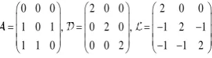
Fig. 1 multi-agent system in this paper

In Fig.1, the triangle “i” represents i-th agent(i=1,2,3). Moreover “

l

” means the leader and the others are followers,

and arrows indicate communication paths. Then, the adjacency matrix , the degree matrix , and the graph Laplacian in

Fig.1 can be obtained as

0 0 0 2 0 0 2 0 0

1 0 1 , 0 2 0 , 1 2 1

1 1 0 0 0 2 1 1 2

     

     

_{ } _{ }  _  _

    _{ } 

     

(6)

( ) ( ) ( ) ( 1, 2,3)

i i i

d

dtx t Ax t Bu t i (7)

wherex t_i( ) nandu t_i( ) mare the vectors of the state and the control input, and the statex t_i( ) nis given by





( ) ( ) ( ) ( ) ( )T

i xi xi yi yi

x t  x t v t x t v t (8)

i.e. the state x_xi( )t (resp.x_yi( )t ) is the position in x-axis (resp. y-axis), and v_xi( )t (resp.v_yi( )t ) is velocity in x-axis (resp.

y-axis) for the i-th agent. In (7),A l n andB l m are the system parameters which are defined as

0 1 0 0 0 0 0 0 0 0 1 0

, 0 0 0 1 0 0 0 0 0 0 0 1

A B

   

   

   

_{ } _{ }

   

   

(9)

Here, in order to consider the relative positions between agents, we introduce the following vectors:



ˆ ˆ



T

i xi xi yi yi

d  d v d v (10)

whered_xi(resp.d_yi) is the desired relative position in x-axis (resp. y-axis) between the i-th agent and the leader agent. Similarly,vˆ_xiandvˆ_yiare the target velocity. Note that one can see that dl 0. Here, we consider the difference between the actual position of the agent (x t_i( )) and the desired relative position between the leader and the follower d_i as a new state of

the system. From (7), the state equation of each follower considering the relative positions from leader to follower is

expressed as



i( ) i





i( ) i



i( ) ( 1, 2.3) d

x t d A x t d Bu t i

dt      (11)

By introducing the additional state vector x t_i( ) described as





( ) ( )

ˆ

( ) ( )

( ) ( )

ˆ

( ) ( )

( ) ( )

xi xi xi

xi xi xi

i i

yi yi yi

yi yi yi

i

x t d x t

v t v v t

x t d x t

v t v v t

x t x t d



   

 _   

   

 _{   } _

   

 _   

   

 (12)

Then one can see from (11) and (12) that the following state equation can be obtained:

( )

( )

( )

i i i

d

dt

x t



Ax t



Bu t

(13)

Summarizing the state equations of all agents, we get the following total system:

( )

_t

( )

_t

( )

d

dt

x t



A x t



B u t

(14)

whereA B x t_t, _t, ( )andu t( )are matrices and vectors given by









3 3

2 3 2 3

0 0 0 0

0 0 , B 0 0

0 0 0 0

( ) ( ) ( ) ( ) , ( ) ( ) ( ) ( )

t t

T T

T T T T T T

l l

A B

A I A A I B B

A B

x t x t x t x t u t u t u t u t

   

   

  _{ }   _{ }

   

   

 

Next, we consider the control input u t( ). Note that consensus problem, “consensus” for agents means that the following

relation for  _i and _j holds:





lim _i( ) _j( ) 0

t x t x t  (16)

If F 2 4 is the consensus gain, it is known that the consensus input forx t_i( ), u_Fi( )t is given by [22].





( ) ( ) ( )

i

Fi i j

j

u t F x t x t







 ₍₁₇₎

In the case of this paper, u_Fi( )t is calculated as follows:

2 2 3

3 2 3

( ) 0

( ) ( ( ) 2 ( ) ( ))

( ) ( ( ) ( ) 2 ( ))

Fl

F l

F l

u t

u t F x t x t x t u t F x t x t x t



   

   

(18)

Namely,





2 3

( ) T ( ) T ( ) T ( )T

F Fl F F

u t  u t u t u t can be represented by the following matrix-vector form:

2

3

0 0 0 ( )

( ) 2 ( ) ( ) ( )

2 ( )

l

F

x t

u t F F F x t F x t

F F F x t

         _  _{ }  _{ }      (19)

Additionally, let uK( )t be the state feedback input for stabilization of the system. By using the feedback gain matrix

2 4

( ) K

u t   , the state feedback input uK( )t can be written as

( ) ( ) ( )

K

u t IK x t (20)

Finally, we introduce a compensation input v(t) and consider the following control input:

( ) ( ) ( ) ( )

( ) ( ) ( ) ( ) ( )

0 0 0 0 0

2 ( ) 2 ( )

2 2

K F

t u t u t u t v t

I K x t F x t v t

K

F K F F x t F F F d v t

F F K F F F F

                _   _  _  _  _{  }  _{ }      (21)

wherev t( )



vlT( )t v₂T( )t vT₃( )t



T. Note that the design method for the compensation input v(t) and the gain matrices

2 4

K



 and

F



2 4 is discussed in the next section. From (14) and (21), we have

2 3

0 0 0 0 0

2 2

2 2

0 0 0 0 ( ) 0 0 0

* 0 ( 2 ) ( ) 2

* * ( 2 ) ( )

( ) ( ) ( ) ( ) l t t t K d

F K F F F F F

dt

F F K F F F F

A BK x t

A BF B K F BF x t BF BF

A BF BF B K F x t

B x t d v t

x t A x t

           _   _  _  _  _ _{  } _ _{ } _              _{  }    _{ }     _{  }             2 3

2 2 2 3

3 3 2 3

0 0

* 0 ( )

2 * *

0 0 ( ) ( )

( ) ( ) (2 )

( ) ( ) ( 2 )

l

K l l

F

F

d B

BF d B v t

BF BF BF d B

A x t Bv t

BF A BF x t Bv t BF d d

BF BF A x t Bv t BF d d

          _        _{ }                       _  _{  }   _ _{ }    _{  }       (22)

From the above, the controller design objective in this study is to derive the consensus gain

F



2 4 , the feedback

gain

K



2 4 and compensation inputv t( ) 6so that the asymptotic stability of the closed-loop system of (22) is

guaranteed.

4.

Main Results

In this section, the design method of the feedback gain

K



2 4 , the consensus gains

F



2 4 and the compensation

input v t_i( ) 2(il, 2,3) is shown.

We give the following theorem for determining these parameters of the overall system (22).

Theorem 1

. Consider the overall system of (14) and the control input of (21). If there exist solutions

S



0

, W_K and

F

W of following LMI condition:

11 12 13

22 23

33

11 12 13

22 33 23

* 0

* *

, 2

,

2 2 ,

K K

T T T T T

K K K

T T T T T T T

K K F F F F

A A BK A A BK BF

SA AS W B BW W B

SA AS W B BW BW W B W B BW

  

 



  

  

 

 _{ }

 

 

 

    

      

        

(23)

then the compensation input

v t

( )

is designed as follows,

2

2 2 3 2 2

2 3

3

3 2 2 3

3 0 ( )

( )

( ) ( ) 2 ( )

( ) ( )

( )

2 ( )

( )

T T l

T T

T T

T T

v t

F B Px t

v t v t Fd dm B Px t

B Px t v t

F B Px t

Fd dm B Px t

B Px t

 

 

  _{ }

 

_{ }   

 

 

 _{  }

 

_{ } 

 

 

 

(24)

where the matrixPis given by

P



S

1and the feedback gain matrixKand the consensus oneFare designed as

1

K

KW S (25)

1

F

FW S (26)

Moreover, by applying the control input of (27) with the compensation input

v t

( )

of (24) the gain matrices K(25) and F (26) to the overall system of (14), asymptotic stability of the closed-loop system of (22) is guaranteed.

Proof: Using a positive definite symmetric matrixPPT 4 4 , we introduce the following quadratic function as a candidate for Lyapunov function:

3

( , )

( ) (

T

) ( )

V x t



x t

I



P x t

(27)

The time derivative of the quadratic function along the trajectory of the closed-loop system of (22) satisfies





3 3

( , ) ( ) (T ) ( ) ( ) (T ) ( )

d d d

V x t x t I P x t x t I P x t

As is well known, the stability condition for the closed-loop system is

( , ) 0

d

dtV x t  (29)

and the time derivative of the quadratic function along the trajectory of the closed-loop system of (22) can be written as

2 2 3 3

3 2 3

3 2 2 3

3

0 0 ( )

( , ) ( ) ( ) (2 ) ( ) ( )

( ) ( 2 )

0 0 ( )

( ) ( ) ( ) ( ) (2 )

( ) T K l F F K l T F F

A Bv t

d

V x t BF A BF x t Bv t BF d d I P x t dt

BF BF A Bv t BF d d

A Bv t

x t I P BF A BF x t Bv t BF d d

BF BF A Bv t B

        _  _ _   _  _{ } _ _{   } _         _  _    _{ }  _

  2 3

2 2 3 2 2 3

3 2 3 3

( 2 )

( ) ( )

*

( ) ( )

( ) ( ) (2 ) ( ) (2 )

( ) ( 2 ) ( )

T T T T T

K K

T T T T

F F

T

F F

l l

T

t t t t

F d d

A P PA F B P F B P x t PBF A P PA F B P PBF x t

PBF A P PA

v t v t

x t P B v t F d d P B v t F d d

v t F d d v t F

       _{ }  _{  } _                              _   _    _{  }  _

  2 3

( )

( 2 )

T x t d d        _{ }  _{  } _   (30)

whereP_t 12 12 is the following symmetric positive definite matrix:

3 0 0 * 0 * * t P

P I P P

P      _{   }     (31)

Here, by introducing the matrix



( , , )

P K F

and the scalar function



( , , ( ))

P F v t

which are defined as





















2 2 3 2 2 3

3 2 3 3 2 3

2 2 3 2

3 2 3

( ) ( )

( , , ( )) ( ) ( ) (2 ) ( ) (2 ) ( )

( ) ( 2 ) ( ) ( 2 )

2 ( ) ( ) 2 ( ) 2 ( )

2 ( ) 2

T

l l

T

t t t t

T T

l l

v t v t

P F v t x t P B v t F d d P B v t F d d x t

v t F d d v t F d d

PB PBv t x t PB PB v t F d d x t

PB PB v t F d d

          _{ } _  _{ } _   _  _  _{  }   _{  }           _   _ 

 _    _Tx t₃( )

(32)

( , , ) *

* *

T T T T T

K K

T T T

F F

T

F F

A P PA F B P F B P

P K F A P PA F B P PBF

A P PA

 _{  }                 (33)

one can see that the stability condition for the closed-loop system of (22) is reduced to

( , ) T( ) ( , , ) ( , , ( )) 0

d_{V x t x t P K F P F v t}

dt     (34)

Namely, if the matrix



( , , )

P K F

is negative definite and



( , , ( ))

P F v t

< 0 are satisfied, then the quadratic function

V x t

( , )

becomes a Lyapunov function. For leader agent, there is no need the compensation input, i.e. v t_l( )0then we have













2 2 2 3 2 2 2 2 2 3 2

3 3 2 3 3 3 3 2 3 3 3

( ) ( ) 0

( ) ( ) (2 ) ( ) ( ) ( ) 2 ( ) ( )

( ) ( ) 2 ( ) ( ) ( ) ( ) 2 ( )

l l

T T T T T T T

T _{T T T T T T}

t PBv t

t PB v t F d d x t v t B Px t d F B Px t d F B Px t

t PB v t F d d x t v t B Px t d F B Px t d F B Px t        _   _      _    _    (35)

where



_i( )t

(

i



l

, 2,3)

is the i-th term in the right-hand side of (32). Sincev t_l( )0, we consider the design problem of 2( )

between the leader and the follower 3, and it is unknown to the follower 2. The follower 2 can obtain the information for the

upper bounddm₃ for the relative position, i.e. dm₃ satisfies

d

₃



dm

₃. Therefore, we consider

2( ) 2 2 3( )

v t   Fd  t (36)

and one can see that for the third term in the right-hand side of



₂( )t in (35) the following inequality holds:

3 2 3 2

3 2

( ) ( )

( )

T T T T

T T

d F B Px t d F B Px t

dm F B Px t

  

 (37)

Thus, by selecting



₃( )t defined as

2

3 3 2 2

2

( )

( ) ( )

( )

T T

T T

F B Px t

t dm B Px t

B Px t

   ₍₃₈₎

we can obtain

2

2 2 2 3 2 2 2 2 2 3 2

2

( )

( ) 2 ( ) ( ) ( ) 2 ( ) ( )

( ) 0

T T

T T T T T T T

T

F B Px t

t d F B Px t dm x t PB B Px t d F B Px t dm F B Px t

B Px t 

 

 

   _{ }  

 

 



(39)

Similarly, we consider the following compensation input for follower 3:

3

( )

2

3 2

( )

v t

 

Fd





t

(40)

For the third term in the right-hand side of



3( )t _{in (35), we find that the inequality}

2 3 2 3

2 3

( ) ( )

( )

T T T T

T T

d F B Px t d F B Px t

dm F B Px t

  

 (41)

is satisfied, and thus



₂( )t is designed as

3

2 2 2 3

3

( )

( ) ( )

( )

T T

T T

F B Px t

t dm B Px t

B Px t

   ₍₄₂₎

Then we can obtain the following inequality:

3( )t 0

  (43)

Consequently, if

v t

( )

is designed as

2

2 2 3 2 2

2 3

3

3 2 2 3 3

0 ( )

( )

( ) ( ) 2 ( )

( ) ( )

( )

2 ( )

( )

T T l

T T

T T

T T

v t

F B Px t

v t v t Fd dm B Px t

B Px t v t

F B Px t

Fd dm B Px t

B Px t

 

 

  _{ }

 

_{ }   

 

 

 _{  }

 

_{ } 

 

 

 

(44)



2 3



( , , ( ))

P F v t

2

( )

t

( )

t

0













(45)

Once again considering the asymptotic stability condition of (34), the quadratic form term of

x t

( )

should satisfy

( ) ( ,

, ) ( )

0

T

x

t



P K F x t



(46)

The inequality of (46) is equivalent to the following condition;

( , , )

P K F

0





(47)

In order to design the consensus gainF, and the feedback gainK, we introduce the symmetric positive definite matrix

S

satisfyingSP1and change of variables W_K KS 2 4 andW_F FS 2 4 . Moreover, pre- and post-multiplying

(47) by

(

I

₃



S

)

, we get.

11 12 13 22 23 33

11

3 3

0 0 0 0

* 0 * * 0

* * _{* *} * *

* 0

* *

( , 2 )

,

( ) ( , , )( )

T T T T T

K K

T T T

F F

T

F F

K K

T T T

K K

A P PA F B P F B P

S S

S A P PA F B P PBF S

S _{A P PA} S

A A BK A A BK BF

SA AS W B BW

I S P K F I S

  

 





 _{  } 

 _{ } 

 _{ } 

_{ }    _{ }

 

 _{ } 

 _  _ 

 

 

_{ }

 

 

    

   

  

12 13

22 33 2 2 , 23

T T K

T T T T T T T

K K F F F F

W B

SA AS W B BW BW W B W B BW

 

  

  

        

(48)

This inequality of (48) is linear matrix inequality (LMI) for

S

, W_K and W_F. If the solution of the LMI of (48) exists,

the asymptotic stability of the closed-loop system of (22) is guaranteed, and the feedback gain K and the consensus gain F can be obtained as

1 1

,

K F

KW S FW S (49)

From the above discussion, the proof of Theorem1 is accomplished.

Remark 1: In this paper, we approached the case of network topology such as fig.1 as an example, but the other

topological structures can be handled if similar theoretical development is applied. However, it is inevitable that LMI will

increase in size and complexity by the number of agents and the topology becomes complicated.

Remark 2: When the relative position between the leader and the follower is considered explicitly, it is often uncertain

or unknown about the relative position between the leader and the other followers. Thus, construction of the state equation is

generally not easy. As a result, there are not much exiting results which have explicitly dealt with the relative position in the

dynamics as far as we know. On the other hand, in this study, it is possible to discuss LMI-based control system design that

clearly indicates relative positional relationship by adding an input using the maximum value of relative distance that is

known when performing the desired formation.

5.

Numerical Simulation

Firstly, by solving LMI (48), we have symmetric positive definite matrices 4 4

S  , P 4 4 and matrices 2 4

K

W  

and 2 4

F

1 3 3

1 3 3

3 3 1

3 3 1

1.1574 4.2577 10 2.0326 10 3.4553 10

4.2577 10 1.1574 3.4553 10 2.0326 10

2.0326 10 3.4553 10 1.1574 4.2577 10

3.4553 10 2.0326 10 4.2577 10 1.1574

S              _{    }  _{    }            _{    }    (50)

1 1 4 3

1 1 3 4

4 3 1 1

3 4 1 1

9.9925 10 3.6760 10 2.3596 10 2.4249 10 3.6760 10 9.9925 10 2.4249 10 2.3462 10 2.3596 10 2.4249 10 9.9925 10 3.6760 10 2.4249 10 2.3462 10 3.6760 10 9.9925 10 P                  _{   }   _{   }            _{   }    (51) 3 18 3

1.1651 1.9053 _{9.7081 10 1.6958 10}

9.7077 10 2.1926 1.1651 1.9053

K

W    _        _

    

  (52)

6 1 6 1

6 1 6 1

6.9246 10 7.9258 10 6.9246 10 5.6843 10 6.9246 10 5.6843 10 6.9246 10 7.9258 10 F W          _{   }    _{   } 

  (53)

Then the feedback gain K 2 4 and the consensus gain F 2 4 can be calculated as

2 3

1

1.8646 2.3321 _{1.4595 10 6.8409 10}

8.2057 10 2.1978 1.8699 2.3327

K __  _  _  _    _   _ (54)

1 1 1 1

1 1 1 1

2.9273 10 7.9213 10 2.1088 10 5.6819 10 2.1088 10 5.6819 10 2.9274 10 7.9213 10 F          _{   }        

  (55)

In this example, initial values for the closed-loop system of (22) are selected as follows;

2 3

5 6 1

2 4 2

(0) , (0) , (0)

3 0 2

2 3 4

l

x x x

            _{ } _{ } _{ }   _          (56)

Furthermore, let r t( )be the leader’s reference input and x t_l( ) be x t_l( )x t_l( )r t( ). In this example, r t( )gives the

leader to go around a circle of radius 3 with 20[s]. Also, give

d

₂ and

d

₃ are so that the followers 2 and 3 leaves the leader

by (2, 2) and (-2, 2).

















2 3

3cos 0.1 _{2 2}

0.3sin 0.1 0 0

( ) , ₂ , ₂ 3sin 0.1

0 0

0.3cos 0.1 t

t

r t d d

t t       _{   } _  _{   }   _{ } _{ }         _{   }   (57)

Additionally, dm₂anddm₃are selected as dm₂ dm₃6.

The simulation result of this numerical example is shown in Figs. 2 - 7. In Figs.2 - 5, show the state trajectory of each

agent and the shape of the formation every 5[s]. Figs.6 and 7 show the time histories of each agent in the x and y-axes, respectively. From Figs.2-5, we can see that the leader follows the given trajectory, and the followers 2 and 3 follow the

desired relative position. Also, from fig.6 and fig.7, looking at the transition of the position coordinates of each agent, it can

be seen that the follower moves away from the leader's movement locus by the desired position as time passes. Namely, it

can be said that the proposed formation control system has been designed, and thus we have shown the effectiveness of the

Fig. 2 Movement of each agent in 0[s] Fig. 3 Movement of each agent in 10[s]

Fig. 4 Movement of each agent in 20[s] Fig. 5 Movement of each agent in 40[s]

Fig.6 Time histories of x (t)_xi Fig.7 Time histories of x (t)_yi

6.

Conclusions

In this paper, we present a design method of an adaptive gain controller considering relative distances between agents

for MASs with leader-follower structure. The proposed adaptive gain controller consists of the state feedback laws with

fixed gains and compensation input with adaptive gains which are adjusted by updating rules. We have shown that the

sufficient conditions for the existence of the proposed adaptive gain controller are reduced to the solvability of LMI, i.e. the

proposed controller can be designed by using software such as MATLAB’s LMI Control Toolbox, Scilab’s LMITOOL and

so on. In the proposed control strategy, there is no need the information on the target value of the other followers and the

information about the upper bound on relative positions is only required. Furthermore, the effectiveness of the proposed

The future research subjects are an extension of the proposed design to such a broad class of systems as discrete-time

systems and output feedback systems. Moreover, for the proposed adaptive gain controller, improvement of transient

performance and guaranteeing disturbance attenuation level are our important future research subjects. Additionally, we will

study the conservativeness of the proposed controller design and extend the proposed controller synthesis to such a broad

class of control systems as a formation for MASs consisting of more general agent’s dynamics with uncertainties and

consensus via output feedback controllers.

Conflicts of Interest

The authors declare no conflict of interest.

References

[1] M. Norton, Modern control engineering, Pergamon Press, 1972.

[2] B. D. O. Anderson and J. B. Moore, Optimal control – linear quadratic method –, Prentice Hall, New Jersey, 1990. [3] K. Zhou, Essentials of robust control, Prentice Hall, 1998.

[4] B. R. Barmish, “Stabilization of uncertain systems via linear control,” IEEE Trans. Automat. Contr., vol. 28, no. 8, pp. 848-850, August 1983.

[5] I. R. Petersen and C. C. Hollot, “A riccati equation approach to the stabilization of uncertain linear systems,” Automatica, vol. 22, no. 4, pp. 397-411, July 1986.

[6] K. Hagino and H. Komoriya, “A Design method of robust control for linear systems,” IEICE Trans. Fundamentals, vol. J72-A, no. 5, pp. 865-868, May 1989. (in Japanese)

[7] P.P. Khargonekar, I.R. Petersen and K. Zhou, “Robust stabilization of uncertain linear systems: quadratic stabilizability and control theory,” IEEE Trans. Automat. Contr., vol. 35, no. 3, pp. 356-361, March 1990.

[8] I. R. Petersen and D. C. McFarlane, “Optimal guaranteed cost control and filtering for uncertain linear systems,” IEEE Trans. Automat. Contr., vol. 39, no. 9, pp. 1971-1977, September 1994.

[9] S. Yamamoto and K. Yamauchi, “A design method of adaptive control systems by a time-varying parameter of robust stabilizing state feedback,” Tran. ISCIE, vol. 12, no. 6, pp. 319-325, May 1999. (in Japanese)

[10] M. Maki and K. Hagino, “Robust control with adaptation mechanism for improving transient behavior,” Int. J. Contr., vol. 72, no. 13, pp. 1218-1226, November 1999.

[11] H. Oya and K. Hagino, “Robust control with adaptive compensation input for linear uncertain systems,” IEICE Trans. Fundamental, of Electronics, Communications and Computer Sciences, vol. E86-A, no. 6, pp. 1517-1524, June 2003. [12] D. D. Siljak, Decentralized control of complex systems, New York, Academic Press., 1991.

[13] R. Olfati-Saber and R. M. Murray, “Consensus problems in networks of agents with switching topology and time-delays,” IEEE Trans. on Automat. Contr., vol. 49, no. 9, pp. 1520-1533, September 2004.

[14] G. Xie and L. Wang, “Consensus control for a class of networks of dynamic agents: fixed topology,” Proc. of the 44th IEEE Conference on Decision and Control, and the European Control Conference 2005, pp.96-101, Seville, SPAIN, December 2005.

[15] Y. Zhang and Y. P. Tian, “Consentability and protocol design of multiagent systems with stochastic switching topology,” Automatica, vol. 45, no. 5, pp. 1195-1201, May 2009.

[16] G. Zhai, S. Okuno, J. IMAE and T. Kobayashi, “A matrix inequality based design method for consensus problems in Multi-Agent Systems,'' Int. J. Appl. Math. Comput. Sci., vol. 19, no. 4, pp. 639-646, April 2009.

[17] W.Ni, and D.Cheng, “Leader-following consensus of multi-agent systems under fixed and switching topologies,” Systems & Control Letters, vol.59, issues.3-4, pp.209-217, March-April 2010.

[18] D.Zhang, Z.Xu, Q.G.Wang, and Y.B.Zhao, “Leader–follower H_∞ consensus of linear multi-agent systems with

aperiodic sampling and switching connected topologies,” ISA Transactions, vol.68, pp.150-159, May 2017 [19] W.He, C.Xu, Q.Han, F.Qian, and Z.Lang, “Finite-time L_2 leader–follower consensus of networked euler–lagrange

systems with external disturbances,” IEEE Transactions on Systems, Man, and Cybernetics: Systems, vol.48 issue 11, pp.1920 – 1928, November 2018.

[21] S. Nagai, H. Oya, T. Kubo, and T. Matsuki, “Synthesis of decentralized variable gain robust controllers for a class of large-scale interconnected systems with mismatched uncertainties,” Int. J. Syst. Science, vol. 48, issue 8, pp. 1616-1623, July 2017.

[22] C. Yoshioka, T. Namerikawa,” Consensus problem for multi-agent system and its application to formation control,” Transaction of The Society of Instrument and Control Engineers, vol. 44, no. 8, pp. 663-669, August 2008. (in Japanese)