Active Learning of Causal Networks with Intervention Experiments and Optimal Designs

Active Learning of Causal Networks

with Intervention Experiments and Optimal Designs

Yang-Bo He [email protected]

Zhi Geng [email protected]

School of Mathematical Sciences, LMAM Peking University

Beijing 100871, China

Editor: Andre Elisseeff

Abstract

The causal discovery from data is important for various scientific investigations. Because we cannot distinguish the different directed acyclic graphs (DAGs) in a Markov equivalence class learned from observational data, we have to collect further information on causal structures from experiments with external interventions. In this paper, we propose an active learning approach for discovering causal structures in which we first find a Markov equivalence class from observational data, and then we orient undirected edges in every chain component via intervention experiments separately. In the experiments, some variables are manipulated through external interventions. We discuss two kinds of intervention experiments, randomized experiment and quasi-experiment. Furthermore, we give two optimal designs of experiments, a batch-intervention design and a sequential-intervention design, to minimize the number of manipulated variables and the set of candidate structures based on the minimax and the maximum entropy criteria. We show theoretically that structural learning can be done locally in subgraphs of chain components without need of checking illegal v-structures and cycles in the whole network and that a Markov equivalence subclass obtained after each inter-vention can still be depicted as a chain graph.

Keywords: active learning, causal networks, directed acyclic graphs, intervention, Markov equiv-alence class, optimal design, structural learning

1. Introduction

obser-vational data. Tian and Pearl (2001a,b) proposed a method of discovering causal structures based on dynamic environment. Tong and Koller (2001) and Murphy (2001) discussed active learning of Bayesian network structures with posterior distributions of structures based on decision theory. In these methods, causal structures are discovered by using additional information from domain experts or experimental data.

Chain graphs were introduced as a natural generalization of DAGs to admit more flexible causal interpretation (Lauritzen and Richardson, 2002). A chain graph contains both directed and undi-rected edges. A chain component of a chain graph is a connected undiundi-rected graph obtained by removing all directed edges from the chain graph. Andersson et al. (1997) showed that DAGs in a Markov equivalence class can be represented by a chain graph. He et al. (2005) presented an ap-proach of structural learning in which a Markov equivalence class of DAGs is sequentially refined into some smaller subclasses via domain knowledge and randomized experiments.

In this paper, we discuss randomized experiments and quasi-experiments of external interven-tions. We propose a method of local orientations in every chain component, and we show theo-retically that the method of local orientations does not create any new v-structure or cycle in the whole DAG provided that neither v-structure nor cycle is created in any chain component. Thus structural learning can be done locally in every chain component without need of checking illegal v-structures and cycles in the whole network. Then we propose the optimal designs of interventional experiments based on the minimax and maximum entropy criteria. These results greatly extend the approach proposed by He et al. (2005). In active learning, we first find a Markov equivalence class from observational data, which can be represented by a chain graph, and then we orient undirected edges via intervention experiments. Two kinds of intervention experiments can be used for orien-tations. One is randomized experiment, in which an individual is randomly assigned to some level combination of the manipulated variables at a given probability. Randomization can disconnect the manipulated variables from their parent variables in the DAG. Although randomized experiments are most powerful for learning causality, they may be inhibitive in practice. The other is quasi-experiment, in which the pre-intervention distributions of some variables are changed via external interventions, but we cannot ensure that the manipulated variables can be disconnected from their parent variables in the DAG, and thus the post-intervention distributions of manipulated variables may still depend on their parent variables. For example, the pre-intervention distribution of whether patients take a vaccine or not may depend on some variables, and the distribution may be changed by encouraging patients with some benefit in the quasi-experiment, but it may still depend on these variables. Furthermore, we discuss the optimal designs by which the number of manipulated vari-ables is minimized or the uncertainty of candidate structures is minimized at each experiment step based on the minimax and the maximum entropy criteria. We propose two kinds of optimal designs: a batch-intervention experiment and a sequential intervention experiment. For the former, we try to find the minimum set of variables to be manipulated in a batch such that undirected edges are all oriented after the interventions. For the latter, we first choose a variable to be manipulated such that the Markov equivalence class can be reduced by manipulating the variable into a subclass as small as possible, and then according to the current subclass, we repeatedly choose a next variable to be manipulated until all undirected edges are oriented.

sequen-tial intervention design. In Section 5, we show simulation results to evaluate the performances of intervention designs proposed in this paper. Conclusions are given in Section 6. Proofs of theorems are given in Appendix.

2. Causal DAGs and Markov Equivalence Class

A graph G can be defined to be a pair G= (V_,E_{), where}V_{={V1,· · ·,Vn}denotes the node set and} E_{denotes the edge set which is a subset of the set}V_×V_{of ordered pairs of nodes. If both ordered}

pairs(Vi,Vj)and(Vj,Vi)are inE, we say that there is an undirected edge between Viand Vj, denoted as Vi−Vj. If (Vi,Vj)∈Eand(Vj,Vi)∈/E, we call it a directed edge, denoted as Vi→Vj. We say that Viis a neighbor of Vj if there is an undirected or directed edge between Viand Vj. A graph is directed if all edges of the graph are directed. A graph is undirected if all edges of the graph are undirected.

A sequence(V1,V2,· · ·,Vk)is called a partially directed path from V1to Vkif either Vi→Vi+1or Vi−Vi+1is in G for all i=1, . . . ,k−1. A partially directed path is a directed path if there is not any undirected edge in the path. A node Viis an ancestor of Vj and Vjis a descendant of Viif there is a directed path from Vito Vj. A directed cycle is a directed path from a node to itself, and a partially directed cycle is a partially directed path from a node to itself.

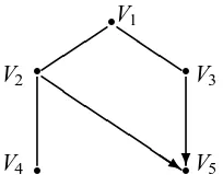
A graph with both directed and undirected edges is a chain graph if there is not any partially directed cycle. Figure 1 shows a chain graph with five nodes. A chain component is a node set whose nodes are connected in an undirected graph obtained by removing all directed edges from the chain graph. An undirected graph is chordal if every cycle of length larger than or equal to 4 possesses a chord.

r

r r

r r

V1

V2 V3

V4 V5

Q_Q Q

? Q_Q

Q_Q Q

QQs

Figure 1: A chain graph G∗depicts the essential graph of G,G1,G2and G3.

A directed acyclic graph (DAG) is a directed graph which does not contain any directed cycle. A causal DAG is a DAG which is used to describe the causal relationships among variables V1,· · ·,Vn. In the causal DAG, a directed edge Vi→Vj is interpreted as that the parent node Viis a cause of the child node Vj, and that Vj is an effect of Vi. Let pa(Vi)denote the set of all parents of Vi and ch(Vi) denote the set of all children of Vi. Letτbe a node subset ofV. The subgraph Gτ= (τ,Eτ)induced by the subsetτhas the node setτand the edge setE_τ=E_∩(τ_×τ_{)which contains all edges falling}

Figure 2 shows four different causal structures of five nodes. The causal graph G in Figure 2 depicts that V1is a cause of V3, which in turn is a cause of V5.

r

r r

r r

V1

V2 V3

V4 V5

+ QQQs

? ? Q_Q Q_Q QQs G r r r r r V1

V2 V3

V4 V5

3 QQQs

? ? Q_Q Q_Q QQs G1 r r r r r V1

V2 V3

V4 V5

3 QQQs 6 ? Q_Q Q_Q QQs G2 r r r r r V1

V2 V3

V4 V5

+ QkQQ

? ?

Q_Q Q_Q

QQs

G3

Figure 2: The equivalence class[G].

A joint distribution P satisfies Markov property with respect to a graph G if any variable of G is independent of all its non-descendants in G given its parents with respect to the joint distribution P. Furthermore, the distribution P can be factored as follows

P(v1,v2,· · ·,vn) = n

∏

i=1

P(vi|pa(vi)),

where vi denotes a value of variable Vi, and pa(vi)denotes a value of the parent set pa(Vi)(Pearl, 1988; Lauritzen, 1996; Spirtes et al., 2000). In this paper, we assume that any conditional indepen-dence relations in P are entailed by the Markov property, which is called the faithfulness assump-tion (Spirtes et al., 2000). We also assume that there are no latent variables (that is, no unmeasured variables) in causal DAGs. Different DAGs may encode the same Markov properties. A Markov equivalence class is a set of DAGs that have the same Markov properties. Let G1∼G2denote that two DAGs G1 and G2 are Markov equivalent, and let [G]denote the equivalence class of a DAG G, that is, [G] ={G0 : G0∼G}. The four DAGs G, G1, G2 and G3 in Figure 2 form a Markov equivalence class[G]. Below we review two results about Markov equivalence of DAGs given by Verma and Pearl (1990) and Andersson et al. (1997).

Lemma 1 (Verma and Pearl, 1990) Two DAGs are Markov equivalent if and only if they have the same skeleton and the same v-structures.

Andersson et al. (1997) used an essential graph G∗to represent the equivalence class[G]. Definition 2 The essential graph G∗= (V_,E∗_{)of G has the same node set and the same skeleton}

as G, whose one edge is directed if and only if it has the same orientation in every DAG in[G]and whose other edges are undirected.

For example, G∗ in Figure 1 is the essential graph of G in Figure 2. The edges V2→V5 and V3→V5in G∗are directed since they have the same orientation for all DAGs of[G]in Figure 2, and other edges are undirected.

Lemma 3 (Andersson et al., 1997) Let G∗be the essential graph of G= (V_,E_{). Then G}∗ _{has the}

(i) G∗is a chain graph,

(ii) G∗_τ is chordal for every chain componentτ, and

(iii) Vi→Vj−Vkdoes not occur as an induced subgraph of G∗.

Suppose that G is an unknown underlying causal graph and that its essential graph G∗= (V_,E₎

has been obtained from observational data, and has k chain components{τ1,· · ·,τk}. Its edge set

E_{can be partitioned into the set}E_{1 of directed edges and the set}E_{2of undirected edges. Let G}∗_τ

denote a subgraph of the essential G∗induced by a chain componentτof G∗. Any subgraph of the essential graph induced by a chain component is undirected. Since all v-structures can be discovered from observational data, any subgraph G0_τ of G0 should not have any v-structure for G0∈[G]. For example, the essential graph G∗ in Figure 1 has one chain componentτ={V1,V2,V3,V4}. It can been seen that G0_τhas no v-structure for G0∈ {G,G1,G2,G3}.

Given an essential graph G∗, we need to orient all undirected edges in each chain component to discover the whole causal graph G. Below we show that the orientation can be done separately in every chain component. We also show that there are neither new v-structures nor cycles in the whole graph as long as there are neither v-structures nor cycles in any chain component. Thus in the orientation process, we only need to ensure neither v-structures nor cycles in any component, and we need not check new v-structures and cycles for the whole graph.

Theorem 4 Letτbe a chain component of an essential graph G∗. For each undirected edge V−U in G∗_τ, neither orientation V →U nor V ←U can create a v-structure with any node W outsideτ,

that is, neither V →U←W nor W →V ←U can occur for any W ∈/τ.

Theorem 4 means that there is not any node W outside the component τ which can build a v-structure with two nodes inτ.

Theorem 5 Letτbe a chain component of G∗. If orientation of undirected edges in the subgraph G∗_τ does not create any directed cycle in the subgraph, then the orientation does not create any directed cycle in the whole DAG.

According to Theorems 4 and 5, we find that the undirected edges can be oriented separately in each chain component regardless of directed and undirected edges in other part of the essential graph as long as neither cycles nor v-structures are constructed in any chain component. Thus the orientation for one chain component does not affect the orientations for other components. The orientation approach and its correctness will be discussed in Section 3.

3. Active Learning of Causal Structures via External Interventions

3.1 Interventions by Randomized Experiments

In this subsection, we conduct interventions as randomized experiments, in which some variables are manipulated from external interventions by assigning individuals to some levels of these variables in a probabilistic way. For example, in a clinical trial, every patient is randomly assigned to a treatment group of Vi=viat a probability P0(vi). The randomized manipulation disconnects the node Vifrom its parents pa(Vi) in the DAG. Thus the pre-intervention conditional probability P(vi|pa(vi)) of Vi=vi given pa(Vi) =pa(vi)is replaced by the post-intervention probability P0(vi)while all other conditional probabilities P(vj|pa(vj))for j6=i are kept unchanged in the randomized experiment. Then the post-intervention joint distribution is

PVi(v1,v2,· · ·,vn) =P

0_(v i)

∏

j6=i

P(vj|pa(vj)),

(Pearl, 1993). From this post-intervention distribution, we have PVi(vi|pa(vi)) =PVi(vi), that is, the

manipulated variable Vi is independent of its parents pa(Vi) in the post-intervention distribution. Under the faithfulness assumption, it is obvious that an undirected edge between Viand its neighbor Vjcan be oriented as Vi←Vjif the post-intervention distribution has Vi Vj, otherwise it is oriented as Vi→Vj, where Vi Vj denotes that Vi is independent of Vj. The orientation only needs an inde-pendence test for the marginal distribution of variables Vi and Vj. Notice that the independence is tested by using only the experimental data without use of the previous observational data.

Let e(Vi)denote the orientation of edges which is determined by manipulating node Vi. If Vi belongs to a chain componentτ(that is, it connects at least one undirected edge), then the Markov equivalence class [G]can be reduced by manipulating Vi to the post-intervention Markov equiva-lence class[G]_e(Vi)

[G]e(Vi)={G

0_∈[G]|G0_{has the same orientation as e(V} i)}.

A Markov equivalence class is split into several subclasses by manipulating Vi, each of which has different orientations e(Vi). Let G∗_e(Vi) denote the post-intervention essential graph which depicts the post-intervention Markov equivalence class [G]e(Vi). We show below that G

∗

e(Vi) also has the

properties of essential graphs.

Theorem 6 Letτbe a chain component of the pre-intervention essential graph G∗and Vibe a node in the componentτ. The post-intervention graph G∗_e(V

i)is also a chain graph, that is, G

∗

e(Vi)has the

following properties:

(i) G∗_e(V

i)is a chain graph,

(ii) G∗_e(V

i)is chordal, and

(iii) Vj→Vk−Vl does not occur as an induced subgraph of G∗_e(Vi).

By Theorem 6, the pre-intervention chain graph is changed by manipulating a variable to an-other chain graph which has less undirected edges. Thus variables in chain components can be manipulated repeatedly until the Markov equivalence subclass is reduced to a subclass with a single DAG, and properties of chain graphs are not lost in this intervention process.

al., 1995; Verma and Pearl, 1990; Castelo and Perlman, 2002). Next we choose a variable Vi to be manipulated from a chain component, and we can orient the undirected edges connecting Viand some other undirected edges whose reverse orientations create v-structures or cycles. Repeating this process, we choose a next variable to be manipulated until all undirected edges are oriented. Below we give an example to illustrate the intervention process.

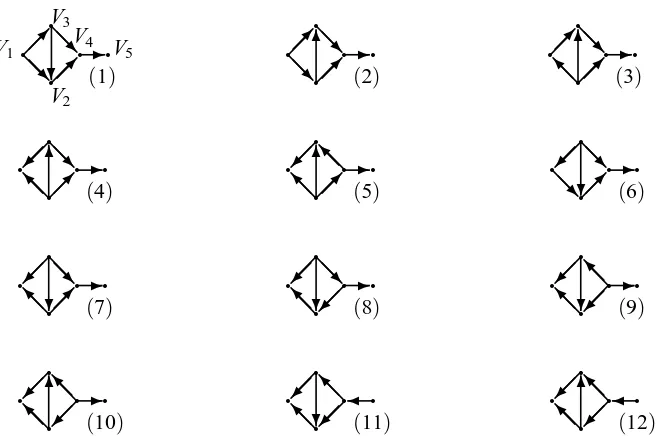
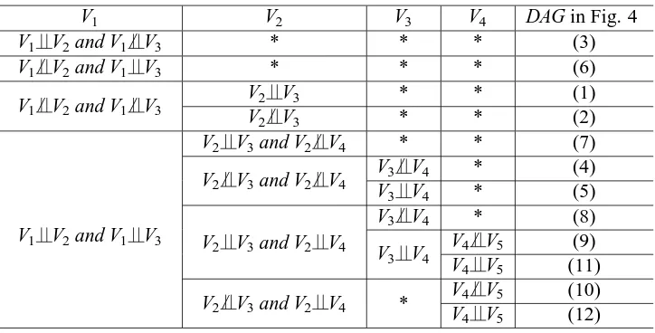
Example 1. Consider an essential graph in Figure 3, which depicts a Markov equivalence class with 12 DAGs in Figure 4. After obtaining the essential graph from observational data, we manipulate some variables in randomized experiments to identify a causal structure in the 12 DAGs. For example, Table 1 gives four possible orientations and Markov equivalence subclasses obtained by manipulating V1. A class with 12 DAGs is split into four subclasses by manipulating V1. The post-intervention subclasses(ii)and(iv)have only a single DAG separately. Notice that undirected edges not connecting V1 can also be oriented by manipulating V1. The subclasses(i)and(iii) are depicted by post-intervention essential graphs (a) and (b) in Table 1 respectively, both of which are chain graphs. In Table 2, the first column gives four possible independence sets obtained by manipulating V1. For the set with V1 V2and V1/ V3, the causal structure is the DAG (3) in Figure 4, and thus we need not further manipulate other variables. For the third set with V1/ V2and V1/ V3, we manipulate the next variable V2. If V2 V3, then the causal structure is the DAG (1), otherwise it is the DAG (2). For the fourth set with V1 V2 and V1 V3, we may need further to manipulate variables V2, V3and V4to identify a causal DAG.

r

r r

r r

V1

V2 V3

V4 V5

@ @_@

@ @_@

Figure 3: An essential graph of DAGs

3.2 Interventions by Quasi-experiments

In the previous subsection we discussed interventions by randomized experiments. Although ran-domized experiments are powerful tools to discover causal structures, it may be inhibitive or im-practical. In this subsection we consider quasi-experiments. In a quasi-experiment, individuals may choose treatments non-randomly, but their behaviors of treatment choices are influenced by experi-menters. For example, some patients may not comply with the treatment assignment from a doctor, but some of them may comply, which is also called an indirect experiment in Pearl (1995).

If we perform an external intervention on Visuch that Vihas a conditional distribution P0(vi|pa(vi)) different from the pre-intervention distribution P(vi|pa(vi))in (1) and other distributions are kept unchanged, then we have the post-intervention joint distribution

PVi(v1,v2,· · ·,vn) =P

0_(v

i|pa(vi))

∏

j6=i

q q q q q V1 V2 V3

V4 _V5

(1)

@_{@R ?}

@_@R

- q q

q

q q

(2)

@_@R6

@_@R

- q q

q

q q

(3)

@ @ I

6@_@R

-q

q q

q q

(4)

@ @ I 6@@R

- q

q q

q q

(5)

@ @ I 6@@I

- q

q q

q q

(6)

@@R ? -@_@R

q

q q

q q

(7)

@@R ? -@ @

I q q

q

q q

(8)

@@R ? -@ @

I q q

q

q q

(9)

@ @ I ?@

@ I -q q q q q

(10)

@ @ I

6@_{I -@} q

q q

q q

(11)

@ @ I ?@

@

I q

q q

q q

(12)

@ @ I

6@_{I @}

Figure 4: All DAGs in the equivalence class given in Figure 3.

No of subclass e(V1)

DAGs in a subclass

post-intervention essential graphs

(i) V2←V1→V3 (1,2) q q q

q q

(a)

V1 _@

@ R

@_@R

-(ii) V2→V1→V3 (3)

(iii) V2→V1←V3

(4,5,

7−12)

q

q q

q q

V1

(b)

@ @ I @@

(iv) V2←V1←V3 (6)

Table 1: The post-intervention subclasses and essential graphs obtained by manipulating V1.

V1 V2 V3 V4 DAG in Fig. 4

V1 V2and V1/ V3 * * * (3)

V1/ V2and V1 V3 * * * (6)

V1/ V2and V1/ V3 V2 V3 * * (1)

V2/ V3 * * (2)

V1 V2and V1 V3

V2 V3and V2/ V4 * * (7)

V2/ V3and V2/ V4

V3/ V4 * (4)

V3 V4 * (5)

V2 V3and V2 V4

V3/ V4 * (8)

V3 V4

V4/ V5 (9)

V4 V5 (11)

V2/ V3and V2 V4 * V4/ V5 (10)

V4 V5 (12)

Table 2: The intervention process to identify a causal structure from the essential graph in Figure 3, where∗means that the intervention is unnecessary.

B6=/0. Below we show a result which can be used to identify the direction of the undirected edge Vi−Vkvia a quasi-experiment of intervention on Vi.

Theorem 7 For a quasi-experiment of intervention on Vi, we have the following properties 1. PVi(vk|B) =P(vk|B)for all vkand B if Vi is a parent of Vk, and

2. PVi(vk) =P(vk)for all vkif Viis a child of Vk.

According to Theorem 7, we can orient the undirected edge Vi−Vk as

1. Vi←Vk if PVi(vk|B)6=P(vk|B)for some vkand B, or

2. Vi→Vk if PVi(vk)6=P(vk)for some vk.

The nonequivalence of pre- and post-intervention distributions is tested by using both experimental data and observational data, which is different from that of randomized experiments.

Example 1 (continued). Consider again the essential graph in Figure 3. We use a quasi-experiment of manipulating V1in order to orient the undirected edges connecting V1(V3−V1−V2). We may test separately four null hypotheses PV1(v2) =P(v2), PV1(v3) =P(v3), PV1(v2|v1,v3,v4) =

P(v2|v1,v3,v4) and PV1(v3|v1,v2,v4) = P(v3|v1,v2,v4) with both observational and experimental

data. We orient V1−V2 as V1→V2 if PV1(v2)6=P(v2), otherwise as V1←V2 (or further check

whether there is a stronger evidence of PV1(v2|v1,v3,v4)6=P(v2|v1,v3,v4)). Similarly we can orient

V1−V3. Finally we obtain four possible orientations as shown in Table 1.

If both PVi(vk) =P(vk) and PVi(vk|B) =P(vk|B) for all vk and B hold for a quasi-experiment,

undirected edge V1−V2cannot be oriented with the intervention on V1with pV1(V1=v)6=p(V1=v)

for v=1 and 2 but pV1(V1=3) =p(V1=3)because we have that pV1(v2) =p(v2)for all v2and that

pV1(v2|B) = p(v2|B)where B={V1}. In a quasi-experiment, an experimenter may not be able to

manipulate V1, and thus this phenomenon can occur. If V1can be manipulated, then the experimenter can choose the distribution of V2to avoid this phenomenon.

4. Optimal Designs of Intervention Experiments

In this section, we discuss the optimal designs of intervention experiments which are used to min-imize the number of manipulated variables or to minmin-imize the uncertainty of candidate structures after an intervention experiment based on some criteria. Since the orientation for one chain compo-nent is unrelated to the orientations for other compocompo-nents, we can design an intervention experiment for each chain component separately. As shown in Section 2, given a chain componentτ, we orient the subgraph overτinto a DAG G_τwithout any v-structure or cycle via experiments of interventions in variables inτ. For simplicity, we omit the subscriptτin this section. In the following subsec-tions, we discuss intervention designs for only one chain component. We first introduce the concept of sufficient interventions and discuss their properties of sufficient interventions, then we present the optimal design of batch interventions, and finally we give the optimal design of sequential in-terventions. For optimizing quasi-experiments of interventions, we assume that intervention on a variable Vi will change the marginal distribution of its child Vj, that is, there is a level vj such that PVi(vj)6=P(vj)for Vi→Vj. Under this assumption, all undirected edges connecting a node Vican

be oriented via a quasi-experiment of intervention on variable Vi. Without the assumption, there may be some undirected edge which cannot be oriented even if we perform interventions in both of its two nodes.

4.1 Sufficient Interventions

It is obvious that we can identify a DAG in a Markov equivalence class if we can manipulate all variables which connect undirected edges. However, it may be unnecessary to manipulate all of these variables. Let

S

= (V1,V2,· · ·,Vk)denote a sequence of manipulated variables. We say that a sequence of manipulated variables is sufficient for a Markov equivalence class[G]if we can identify one DAG from all possible DAGs in[G]after these variables in the sequence are manipulated. That is, we can orient all undirected edges of the essential graph G∗no matter which G in[G]is the true DAG. There may be several sufficient sequences for a Markov equivalence class[G].

Let g denote the number of nodes in the chain component, and h the number of undirected edges within the component. Then there are at most 2hpossible orientation of these undirected edges, and thus there are at most 2h DAGs over the component in the Markov equivalence class. Given a permutation of nodes in the component, a DAG can be obtained by orienting all undirected edges backwards in the direction of the permutation, and thus there are at most min{2h,g!}DAGs in the class.

Theorem 8 If a sequence

S

= (V1,V2,· · ·,Vk)of manipulated variables is sufficient, then any per-mutation of

S

is also sufficient.

is also sufficient. Manipulating Vi, we obtain a class E(Vi) ={e(Vi)} of orientations (see Table 1 as an example). Given an orientation e(Vi), we can obtain the class[G]e(Vi) by (3). We say that

e(V1, . . . ,Vk) ={e(V1), . . . ,e(Vk)}is a legal combination of orientations if there is not any v-structure or cycle formed and there is not any undirected edge oriented in two different directions by these orientations. For a set

S

= (V1, . . . ,Vk)of manipulated variables, the Markov equivalence class is reduced into a class

[G]e(V1,...,Vk)= [G]e(V1)∩. . .∩[G]e(Vk)

for a legal combination e(V1, . . . ,Vk)of orientations. If[G]e(V1,...,Vk)has only one DAG for all

possi-ble legal combinations e(V1, . . . ,Vk)∈E(V1)×. . .×E(Vk), then the set

S

is a sufficient set for iden-tifying any DAG in[G]. LetS_{denote the class of all sufficient sets, that is,}S_={

S

_:

S

_{is sufficient}.}

We say that a sequence

S

is minimum if any subset of

S

is not sufficient.

Theorem 9 The intersection of all sufficient sets is an empty set, that is,T

S∈S

S

=∅. In addition, the intersection of all minimum sufficient sets is also an empty set.

From Theorem 9, we can see that there is not any variable that must be manipulated to identify a causal structure. Especially, any undirected edge can be oriented by manipulating either of its two nodes.

4.2 Optimization for Batch Interventions

We say that an intervention experiment is a batch-intervention experiment if all variables in a suf-ficient set

S

are manipulated in a batch to orient all undirected edges of an essential graph. Let |

S

|denote the number of variables in

S

. We say that a batch intervention design is optimal if its sufficient set

So

has the smallest number of manipulated variables, that is,|

So

|=min{|

S

|:

S

∈S_}.

Given a Markov equivalence class[G], we try to find a sufficient set S which has the smallest num-ber of manipulated variables for identifying all possible DAGs in the class[G]. Below we give an algorithm to find the optimal design for batch interventions, in which we first try all sets with a sin-gle manipulated variable, then try all sets with two variables, and so on, until each post-intervention Markov equivalence class has a single DAG.

Given a Markov equivalence class [G], we manipulate a node V and obtain an orientation of some edges, denoted by e(V). The class [G]is split into several subclasses, denoted by [G]_e(V) for all possible orientations e(V). Let[G]e(V1,V2)denote a subclass with an orientation obtained by

manipulating V1 and V2. The following algorithm 1 performs exhaustive search for the optimal design of batch interventions. Before calling Algorithm 1, we need to enumerate all DAGs in the class [G], and then we can easily find [G]_e(Vi) according to (3). There are at most min{g!,2h} DAGs in the class[G], and thus the upper bound of the complexity for enumerating all{[G]e(Vi)}is

min{g!,2h}. We may be able to have an efficient method to find all{[G]e(Vi)}using the structure of

Algorithm 1 Algorithm for finding the optimal designs of batch interventions

Input: A chain graph G induced by a chain componentτ={V1, . . . ,Vg}, and[G]e(Vi)for all e(Vi)

and i.

Output: All optimal designs of batch interventions.

Initialize the size k of the minimum intervention set as k=0. repeat

Set k=k+1.

for all possible variable subsets

S

={Vi1, . . . ,Vik}do

if|[G]e(S)|=1 for all possible legal combination e(

S

)of orientations then return the minimum sufficient set

S

end if end for

until find some sufficient sets

Algorithm 1 exhaustively searches all combinations of manipulated variables to find the mini-mum sufficient sets, and its complexity is O(g!), although Algorithm 1 may stop whenever it finds some minimum sets. The calculations in Algorithm 1 are only simple set operations

[G]e(S)= [G]e(V_i1)∩. . .∩[G]e(V_ik),

where all[G]e(Vi)have been found before calling Algorithm 1. Notice that a single chain component

usually has a size g much less than the total number n of variables. Algorithm 1 is feasible for a mild size g. A more efficient algorithm or a greedy method is needed for a large g and h. In this case, there are too many DAGs to enumerate. We can first take a random sample of DAGs from the class[G]with the simulation method proposed in the next subsection, and then we use the sample approximately to find an optimal design.

A possible greedy approach is to select a node to be first manipulated from the chain component which has the largest number of neighbors such that the largest number of undirected edges are oriented by manipulating it, and then delete these oriented edges. Repeat this process until there is not any undirected edge left. But there are cases where the sufficient set obtained from the greedy method is not minimum.

Example 1 (continued). Consider the essential graph in Figure 3, which depicts a Markov equivalence class with 12 DAGs in Figure 4. From Algorithm 1, we can find that{1,2,4},{1,3,4}, {2,3,4}and{2,3,5}are all the minimum sufficient sets. The greedy method can obtain the same minimum sufficient sets for this example.

4.3 Optimization for Sequential Interventions

The optimal design of batch interventions presented in the previous subsection tries to find a min-imum sufficient set

S

before any variable is manipulated, and thus it cannot use orientation results obtained by manipulating the previous variables during the intervention process. In this subsection, we propose an experiment of sequential interventions, in which variables are manipulated sequen-tially. Let

S

(t)denote the set of variables that have been manipulated before step t and

S

(0)=/0. At step t of the sequential experiment, according to the current Markov equivalence class[G]_e(S(t−1)₎

based on some criterion. We consider two criteria for choosing a variable. One is the minimax crite-rion based on which we choose a variable V such that the maximum size of subclasses[G]_e(S(t)₎for

all possible orientations e(

S

(t)_{)is minimized. The other is the maximum entropy criterion based on} which we choose a variable V such that the following entropy is maximized for any V in the chain componentτ

HV =−

M

∑

i=1 li Llog

li L,

where li denotes the number of possible DAGs of the chain component with the ith orientation e(V)i obtained by manipulating V , L =∑ili and M is the number of all possible orientations e(V)1, . . . ,e(V)M obtained by manipulating V . Based on the maximum entropy criterion, the post-intervention subclasses have sizes as small as possible and they have sizes as equal as possible, which means uncertainty for identifying a causal DAG from the Markov equivalence class is mini-mized by manipulating V . Below we give two examples to illustrate how to choose variables to be manipulated in the optimal design of sequential interventions based on the two criteria.

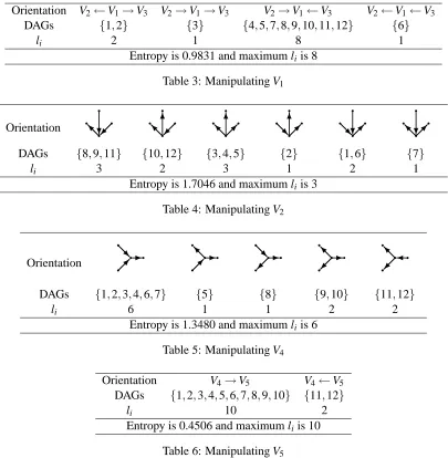
Example 1 (continued). Consider again the essential graph in Figure 3, which depicts a Markov equivalence class with 12 DAGs in Figure 4. Tables 3 to 6 show the results for manipulating one of variables V1, V2(symmetry to V3), V4and V5respectively in order to distinguish the possible DAGs in Figure 4. The first row in these tables gives possible orientations obtained by manipulating the corresponding variable. The second row gives DAGs obtained by the orientation, where numbers are used to index DAGs in Figure 4. The third row gives the number liof DAGs of this chain component for the ith orientation. The entropies for manipulating V1, . . . ,V5are 0.9831, 1.7046, 1.7046, 1.3480, 0.4506, respectively. Based on the maximum entropy criterion, we choose variable V2or V3 to be manipulated first. The maximum numbers li of DAGs for manipulating one of V1, . . . ,V5 are 8, 3, 3, 6, 10, respectively. Based on the minimax criterion, we also choose variable V2 or V3 to be manipulated first.

Although the same variable V2 or V3 is chosen to be manipulated first in the above example, in general, the choice may be different based on the two criteria. The minimax criterion tends to be more conservative, and the entropy criterion tends to be more uniform. For example, consider two interventions for an equivalence class with 10 DAGs: one splits the class into 8 subclasses with the numbers(l1, . . . ,l8) = (1,1,1,1,1,1,1,3)of DAGs, the other splits it into 5 subclasses with the numbers of DAGs equal to (2,2,2,2,2). Then the minimax criterion chooses the second intervention, while the maximum entropy criterion chooses the first intervention.

To find the number (li for i=1,· · ·,M), we need to enumerate all DAGs in the class[G]and then count the number li of DAGs with the same orientations as e(V)i. As discussed in Section 4.2, the upper bound of the complexity for calculating all li is O(min{g!,2h}). Generally the size g of a chain component is much less than the number n of the full variable set and the number h of undirected edges in a chain component is not very large. In the following example, we show a special case with a tree structure, where the calculation is easy.

Orientation V2←V1→V3 V2→V1→V3 V2→V1←V3 V2←V1←V3 DAGs {1,2} {3} {4,5,7,8,9,10,11,12} {6}

li 2 1 8 1

Entropy is 0.9831 and maximum liis 8

Table 3: Manipulating V1

Orientation q q q q @ @

I? q q

q

q

@ @

I6 q q q

q

@ @

I6 q q q

q

@@R6 q q q

q

@@R? q q q

q

@ @ I?

DAGs {8,9,11} {10,12} {3,4,5} {2} {1,6} {7}

li 3 2 3 1 2 1

Entropy is 1.7046 and maximum liis 3

Table 4: Manipulating V2

Orientation

q q

q q

@@R

- q q q q @ @ I - q q q q @ @ R -q q q q @ @ I -q q q q @ @ I

DAGs {1,2,3,4,6,7} {5} {8} {9,10} {11,12}

li 6 1 1 2 2

Entropy is 1.3480 and maximum liis 6

Table 5: Manipulating V4

Orientation V4→V5 V4←V5 DAGs {1,2,3,4,5,6,7,8,9,10} {11,12}

li 10 2

Entropy is 0.4506 and maximum liis 10

Table 6: Manipulating V5

determinate all orientations of edges connecting V , and thus all subtrees that are emitted from V can be oriented, but only one subtree with V as a terminal cannot be oriented. Suppose that node V connects M undirected edges, and let li denote the number of nodes in the ith subtree connecting V for i=1, . . . ,M. Since each node in the ith subtree may be the root of this subtree, there are li possible orientations for the ith subtree. Thus we have the entropy for manipulating V

HV =−

M

∑

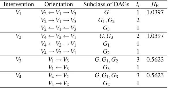
i=1 li Llog li L.

orientation and the last column gives the entropy for each intervention. From Table 7, we can see that manipulating V1or V2has the maximum entropy and the minimax size.

Intervention Orientation Subclass of DAGs li HV V1 V2←V1→V3 G 1 1.0397

V2→V1→V3 G1,G2 2

V2←V1←V3 G3 1

V2 V4←V2←V1 G,G3 2 1.0397

V4←V2→V1 G1 1

V4→V2→V1 G2 1

V3 V1→V3 G,G1,G2 3 0.5623

V1←V3 G3 1

V4 V4←V2 G,G1,G3 3 0.5623

V4→V2 G2 1

Table 7: Manipulating variables in a chain component with a tree structure.

An efficient algorithm or an approximate algorithm is necessary when both g and h are very large. A simulation algorithm can be used to estimate li/L. In this simulation method, we randomly take a sample of DAGs without any v-structure from the class [G]. To draw such a DAG, we randomly generate a permutation of all nodes in the class, orient all edges backwards in the direction of the permutation, and keep only the DAG without any v-structure. There may be some DAGs in the sample which are the same, and we keep only one of them. Then we count the number l_i0 of DAGs in the sample which have the same orientation as e(V)i. We can use l0i/L0 to estimate li/L, where L0=∑il_i0. When the sample size tends to infinite, all DAGs in the class can be drawn, and then the estimate l_i0/L0 tends to li/L. Another way to draw a DAG is that we randomly orient each undirected edge of the essential graph, but we need to check whether there is any cycle besides v-structure.

5. Simulation

In this section, we use two experiments to evaluate the active learning approach and the optimal designs via simulations. In the first experiment, we evaluate a whole process of structural learning and orientation in which we first find an essential graph using the PC algorithm and then orient the undirected edges using the approaches proposed in this paper. In the second experiment, we compare various designs for orientations starting with the same underlying essential graph. For both experiments, the DAG (1) in Figure 4 is used as the underlying DAG and all variables are binary. Its essential graph is given in Figure 3 and there are other 11 DAGs which are Markov equivalent to the underlying DAG (1), as shown in Figure 4. This essential graph can also be seen as a chain component of a large essential graph. All conditional probabilities P(vj|pa(vj))are generated from the uniform distribution U(0,1). We repeat 1000 simulations with the sample size n=1000.

intervention experiments, we run simulations for various combinations of significance levelsαI= 0.01,0.05,0.10,0.15,0.20,0.30 and sample sizes nI=50,100,200,500 in intervention experiments. To compare the performance of the experiment designs, we further give the numbers of manipulated variables that are necessary to orient all undirected edges of the same essential graphs in various in-tervention designs. We run the simulations using R 2.6.0 on an Intel(R) Pentium(R) M Processor with 2.0 GHz and 512MB RAM and MS XP. It takes averagely 0.4 second of the processor time for a simulation, and each simulation needs to finish the following works: (1) generate a joint distribu-tion and then generate a random sample of size n=1000, (2) find an essential graph using the PC algorithm, (3) find an optimal design, and (4) repeatedly generate experimental data of size nIuntil identifying a DAG.

To make the post-intervention distribution P0(vi|pa(vi))different from the pre-intervention P(vi|pa(vi)), we use the post-intervention distribution of the manipulated variable Vias follows

P0(vi|pa(vi)) =P0(vi) =

1, P(vi)≤0.5; 0, otherwise.

To orient an undirected edge Vi−Vj, we implemented both the independence test of the manipulated Viand its each neighbor variable Vjfor randomized experiments and the equivalence test of pre- and post-intervention distributions (i.e., PVi(vj) =P(vj) for all vj) in our simulations. Both tests have

the similar results and the independence test is little more efficient than the equivalence test. To save space, we only show the simulation results of orientations obtained by the equivalence test and the optimal design based on the maximum entropy criterion in Table 8, and other designs have the similar results of orientations.

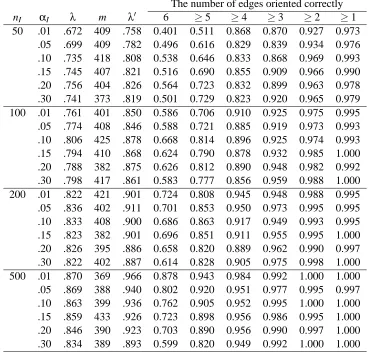
nI. For example,αI=0.20 is the best for nI=50,αI=0.10 for nI=100,αI=0.05 for nI=200, αI=0.01 for nI=500.

The number of edges oriented correctly

nI αI λ m λ0 6 ≥5 ≥4 ≥3 ≥2 ≥1

50 .01 .672 409 .758 0.401 0.511 0.868 0.870 0.927 0.973 .05 .699 409 .782 0.496 0.616 0.829 0.839 0.934 0.976 .10 .735 418 .808 0.538 0.646 0.833 0.868 0.969 0.993 .15 .745 407 .821 0.516 0.690 0.855 0.909 0.966 0.990 .20 .756 404 .826 0.564 0.723 0.832 0.899 0.963 0.978 .30 .741 373 .819 0.501 0.729 0.823 0.920 0.965 0.979 100 .01 .761 401 .850 0.586 0.706 0.910 0.925 0.975 0.995 .05 .774 408 .846 0.588 0.721 0.885 0.919 0.973 0.993 .10 .806 425 .878 0.668 0.814 0.896 0.925 0.974 0.993 .15 .794 410 .868 0.624 0.790 0.878 0.932 0.985 1.000 .20 .788 382 .875 0.626 0.812 0.890 0.948 0.982 0.992 .30 .798 417 .861 0.583 0.777 0.856 0.959 0.988 1.000 200 .01 .822 421 .901 0.724 0.808 0.945 0.948 0.988 0.995 .05 .836 402 .911 0.701 0.853 0.950 0.973 0.995 0.995 .10 .833 408 .900 0.686 0.863 0.917 0.949 0.993 0.995 .15 .823 382 .901 0.696 0.851 0.911 0.955 0.995 1.000 .20 .826 395 .886 0.658 0.820 0.889 0.962 0.990 0.997 .30 .822 402 .887 0.614 0.828 0.905 0.975 0.998 1.000 500 .01 .870 369 .966 0.878 0.943 0.984 0.992 1.000 1.000 .05 .869 388 .940 0.802 0.920 0.951 0.977 0.995 0.997 .10 .863 399 .936 0.762 0.905 0.952 0.995 1.000 1.000 .15 .859 433 .926 0.723 0.898 0.956 0.986 0.995 1.000 .20 .846 390 .923 0.703 0.890 0.956 0.990 0.997 1.000 .30 .834 389 .893 0.599 0.820 0.949 0.992 1.000 1.000

Table 8: The simulation results

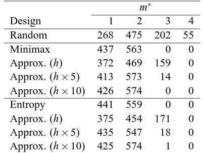
example, the sample sizes of DAGs from the initial essential graph[G]with h=6 undirected edges are 6, 30 and 60, respectively. As the sample size increases, the distribution of the manipulated variable numbers tends to the distribution for the exact minimax design. The optimal sequential design based on the maximum entropy criterion has a very similar performance as that based on the minimax criterion, as shown in the bottom of Table 9. According to Table 9, all of the sequential intervention designs (Random, Minimax, Entropy and their approximations) are more efficient than the batch design, and the optimal designs based on the minimax and the maximum entropy criteria are more efficient than the random design.

m∗

Design 1 2 3 4

Random 268 475 202 55 Minimax 437 563 0 0 Approx. (h) 372 469 159 0 Approx. (h×5) 413 573 14 0 Approx. (h×10) 426 574 0 0 Entropy 441 559 0 0 Approx. (h) 375 454 171 0 Approx. (h×5) 435 547 18 0 Approx. (h×10) 425 574 1 0 m∗denotes the number of manipulated variables Table 9: The frequencies of the numbers of interventions

6. Conclusions

criteria for optimal sequential designs, the minimax and the maximum entropy criteria. The exact, approximate and greedy methods are presented for finding the optimal designs.

The scalability of the optimal designs proposed in this paper depends only on the sizes of chain components but does not depend on the size of a DAG since the optimal designs are performed separately within every chain component. As discussed in Section 4, the optimal designs need to find the number of possible DAGs in a chain component, which has a upper bound min{2h,g!}. When both the number h of undirected edges and the number g of nodes in a chain component are very large, instead of using the optimal designs, we may use the approximate designs via sampling DAGs. We checked several standard graphs found at the Bayesian Network Repository (http://compbio.cs.huji.ac.il/Repository/). We extracted their chain components and found that most of their chain components have tree structures and their sizes are not large. For example, ALARM with 37 nodes has 4 chain components with only two nodes in each component, HailFinder with 56 nodes has only one component with 18 nodes, Carpo with 60 nodes has 9 components with at most 7 nodes in each component, Diabets with 413 nodes has 25 components with at most 3 nodes, and Mumin 2 to Mumin 4 with over 1000 nodes have at most 21 components with at most 35 nodes. Moreover, all of those largest chain components have tree structures, and thus we can easily carry out optimal designs as discussed in Example 2.

In this paper, we assume that there are no latent variables. Though the algorithm can orient the edges of an essential graph and output a DAG based on a set of either batch or sequential interventions, the application of the method for learning causality in the real word is pretty limited because latent or hidden variables are typically present in real-world data sets.

Acknowledgments

We would like to thank the guest editors and the three referees for their helpful comments and suggestions that greatly improved the previous version of this paper. This research was supported by Doctoral Program of Higher Education of China (20070001039), NSFC (70571003, 10771007, 10431010), NBRP 2003CB715900, 863 Project of China 2007AA01Z43, 973 Project of China 2007CB814905 and MSRA.

Appendix A. Proofs of Theorems

Before proving Theorems 4 and 5, we first give a lemma which will be used in their proofs.

Lemma 10 If a node V∈V_{is a parent of a node U in a chain component}τ_{of G}∗_{(i.e.,(V→U)∈G}∗

, U∈τ, V ∈V_{and V ∈/}τ_{), then V is a parent of all nodes in}τ_{(i.e.,(V →W)∈G for any W ∈}τ_).

Proof By (iii) of Lemma 3, V →U W does not occur in any induced subgraph of G∗. Thus for any neighbor of U in the chain componentτ, W and V must be adjacent in G∗. Because V ∈/τ, the edge between V and W is directed. There are two alternatives as shown in Figures 5 and 6 for the subgraph induced by{V,U,W}.

r

r r

V

U W

+ QQQs

Figure 5: SG1

r

r r

V

U W

+ QkQQ

Figure 6: SG2

r

r r

V

U W

+ QkQQ

Figure 7: SG3

of all other variables inτ.

Proof of Theorem 4. According to Lemma 10, if a node W outside a componentτpoints at a node V inτ, then W must point at each node U inτ. Thus W , V and U cannot form a v-structure.

Proof of Theorem 5. Suppose that Theorem 5 does not hold, that is, there is a directed path

V1→ · · · →Vkin Gτwhich is not a directed cycle, but W1→ · · · →Wi→V1→ · · · →Vk→Wi+1→

· · · →W1is a directed cycle, where Wi∈/τ. We denote this cycle as DC. From Lemma 10, Wimust

also be a parent of Vk, and thus W1→ · · · →Wi→Vk→Wi+1→ · · · →W1is also a directed cycle, denoted as DC0. Now, every edge of DC0 is out of Gτ. Similarly, we can remove all edges in other chain components from DC0and keep the path being a directed cycle. Finally, we can get a directed cycle in the directed subgraph of G∗. It contradicts the fact that G∗is an essential graph of a DAG. So we proved Theorem 5.

To prove Theorem 6, we first present an algorithm for finding the post-intervention essential graph G∗_e(V) via the orientation e(V), then we show the correctness of the algorithm using several lemmas, and finally we give the proof of Theorem 6 with G∗_e(V)obtained by the algorithm. In order to prove that G∗_e(V)is also a chain graph, we introduce an algorithm (similar to Step D of SGS and the PC algorithm in Spirtes et al., 2000) for constructing a graph, in which some undirected edges of the initial essential graph are oriented with the information of e(V). Letτbe a chain graph of G∗, V ∈τand e(V)be an orientation of undirected edges connecting V .

Algorithm 2 Find the post-intervention essential graph via orientation e(V) Input: The essential graph G∗and e(V)

Output: The graph H

Orient the undirected edges connecting V in the essential graph G∗according to e(V)and denote the graph as H.

Repeat the following two rules to orient some other undirected edges until no rules can be applied: (i) if V1→V2−V3∈H and V1 and V3 are not adjacent in H, then orient V2−V3as V2→V3and update H;

(ii) if V1→V2→V3∈H and V1−V3∈H, then orient V1−V3as V1→V3and update H. return the graph H

Proof If there is a DAG G0∈[G]such that I=G0_τ, we have from Lemma 1 that I is a DAG with the same skeleton as G∗_τ and without v-structures.

Let I be a DAG with the same skeleton as G∗_τ and without v-structures, and G0be any DAG in the equivalence class[G]. We construct a new DAG I0from G0by substituting the subgraph G0_τof G0 with I. I0has the same skeleton as G0. From Theorems 4 and 5, I0 has the same v-structures as G0. Thus I0is equivalent to G0and I0∈[G].

Lemma 12 Let H be a graph constructed by Algorithm 2. Then H is a chain graph.

Proof If H is not a chain graph, there must be a directed cycle in subgraph H_τ for some chain component of G∗. Moreover, G∗_τ is chordal and H⊂G∗, and thus H_τis chordal too. So we can get a three-edge directed cycle in Hτas given in Figure 8 or 9.

r r r d b c

+ QQQ

Figure 8: SG6

r r r d b c

+ QkQQ

Figure 9: SG61

If Figure 9 is a subgraph of H obtained at some step of Algorithm 2, then the undirected edge b c is oriented as b←c according to Algorithm 2. Thus only Figure 8 can be a subgraph of H.

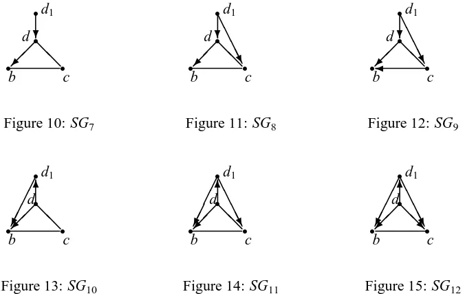
According to Lemma 10, we have that the directed edge d→b is not in G∗. Since all edges connecting a have been oriented in Step 1 of Algorithm 2, d→ b is not an edge connecting a. So d→b must be identified at step 2 of Algorithm 2. There are two situations, one is to avoid a v-structure as shown in Figure 10, the other is to avoid a directed cycle as Figure 13.

r r r r b c d d1 @ @ ?

Figure 10: SG7

r r r r b c d d1 @ @ ? A A AAU

Figure 11: SG8

r r r r b c d d1 @@ ? A A AAU

Figure 12: SG9

r r r r b c d d1 @ @ 6

Figure 13: SG10

r r r r b c d d1 @ @ 6 A A AAU

Figure 14: SG11

r r r r b c d d1 @ @ R 6 A A AAU

Figure 15: SG12

In the first case as Figure 10, if d→b is the first edge oriented at Step 2 of Algorithm 2, we have d1=a. Because b and a are not adjacent, and d c is an undirected edge in H, we have that d1→c must be in H as Figure 11, where d1=a. Now we consider the subgraph b c←d1. According to the rules (i) and (ii) in Algorithm 2, we have that b←c is in G∗_e(a)as Figure 12, which contradicts the assumption that b c∈H.

In the second case as Figure 13, if d→b is the first edge oriented at Step 2 of Algorithm 2, we have d1=a.

Considering the structure d1 →b c and that d c is an undirected edge in H, we have that d1→c must be in H as Figure 14. Now we consider the subgraph of{d,d1,c}. By Algorithm 2,

d→c is in H as Figure 15, which contradicts the assumption that d c∈H. Thus we have that

the first edge oriented at Step 2 of Algorithm 2 is not in any directed cycle. Suppose that the first k oriented edges at Step 2 of Algorithm 2 are not in any directed cycle. Then we want to prove that the(k+1)th oriented edge is also not in a directed cycle.

Let d→b be the(k+1)th oriented edge at Step 2 of Algorithm 2, and Figure 8 be a subgraph of H. There are also two cases as Figures 10 and 13 for orienting d→b.

In the case of Figure 10, since d1→d is in the first k oriented edges and d c∈H, we have that d1→c must be in H. We also get that b←c must be in H as Figure 12, which contradicts the assumption that b c∈H.

In the case of Figure 10, since d1→b and d→d1are in the first k oriented edges and b c∈H, we have that d1→c must be in H. We also get that d←c must be in H as Figure 15, which contra-dicts the assumption that d c∈H. So the(k+1)th oriented edge is also not in any directed cycle. Now we can get that every directed edge in H_τ is not in any directed cycle. It implies that there are no directed cycles in Hτ, and thus H is a chain graph.

Lemma 13 Let G∗_e(V)be the post intervention essential graph with the orientation e(V)and H be the graph constructed by Algorithm 2. We have G∗_e(V)=H.

Proof We first prove G∗_e(a)⊆H. We just need to prove that all directed edges in H must be in G∗_e(a). We use induction to finish the proof.

After Step 1 of Algorithm 2, all directed edges in H are in G∗_e(a). We now prove that the first directed edge oriented at Step 2 of Algorithm 2, such as b←c, is in G∗_e(a). Because b←c must be oriented by the rule (i) of Algorithm 2, there must be a node d∈/τ such that b c←d is the subgraph of H. So b←c←d must be a subgraph in each G0∈G_e∗_(a). Otherwise, b→c←d forms a v-structure such that G0∈/[G]. Thus we have b←c∈G∗_e(a).

Suppose that the first k oriented edges at Step 2 of Algorithm 2 are in G∗_e(a). We now prove that the(k+1)th oriented edge at Step 2 of Algorithm 2 is also in G∗_e(a). Denoting the(k+1)th oriented edge as l←h, according to the rules in Algorithm 2, there are two cases to orient l←h as shown in Figures 16 and 17.

r

r r

f

l h

Q QQs

Figure 16: SG4

r

r r

f

h l

+ QkQQ

In Figure 16, because f →h is in every DAG G0∈G∗_e(a), in order to avoid a new v-structure, we have that l←h must be in every DAG G0∈G∗_e(a). Thus we have l←h∈G∗_e(a). In Figure 17, because l→ f and f →h are in every DAG G0∈G∗_e(a), in order to avoid a directed cycle, we have that h←l must be in every DAG G0 ∈G∗_e(a). Thus we have h←l∈G∗_e(a). Now we get that the (k+1)th oriented edge at Step 2 of Algorithm 2 is also in G∗_e(a). Thus all directed edges in H are also in G∗_e(a)and then we have G∗_e(a)⊆H.

Because H is a chain graph by Lemma 12, we also have H⊆G∗. By Lemma 11, for any undi-rect edge a b of H_τ whereτis a chain component of H, there exist G1 and G2∈G∗_e(a)such that a→b occurs in G1 and a←b occurs in G2. It means that a b also occurs in G∗_e(a). So we have H⊆G∗_e(a), and then G∗_e(a)=H.

Proof of Theorem 6. By definition of G∗_e(V), we have that G∗_e(V) has the same skeleton as the essential graph G∗and contains all directed edges of G∗. That is, all directed edges in G∗are also directed in G∗_e(V). So property 2 of Theorem 6 holds. Property 3 of Theorem 6 also holds because all DAGs represented by G∗_e(V)are Markov equivalent. From Lemmas 12 and 13, we can get that G∗_e(V)is a chain graph.

Proof of Theorem 7. We first prove property 1. Let C=ch(Vk)\τ. Then B=ne(Vk)\C contains all parents of Vk and the children of Vk inτ. Let A=An({B,Vk})be the ancestor set of all nodes in{B,Vk}. Since Vi is a parent of Vk for property 1, we have Vi∈A. The post-intervention joint distribution of A is

PVi(A) =P

0_(v

i|pa(vi))

∏

vj∈A\Vi

P(vj|pa(vj)). (1)

Let U=A\{B,Vk}. Then we have from the post-intervention joint distribution (1)

PVi(vk|B) =

∑UP0(vi|pa(vi))∏vj∈A\ViP(vj|pa(vj)))

∑U,VkP

0_(vi|pa(v

i))∏Vj∈A\ViP(vj|pa(vj))

= ∑UP

0_(v

i|pa(vi))∏vj∈A\{ch(Vk)∩τ,Vk}P(vj|pa(vj))∏vj∈{ch(Vk)∩τ,Vk}P(vj|pa(vj))

∑U,VkP

0_(v

i|pa(vi))∏vj∈A\{ch(Vk)∩τ,Vk}P(vj|pa(vj))∏vj∈{ch(Vk)∩τ,Vk}P(vj|pa(vj)) ,

where∑U denotes a summation over all variables in the set U .

Below we want to factorize the denominator into a production of summation over U and sum-mation over Vk. First we show that the factor P0(vi|pa(vi))∏vj∈A\{ch(Vk)∩τ,Vk}P(vj|pa(vj))does not

contain Vk because Vk appears only in the conditional probabilities of ch(Vk) and the conditional probability of Vk. Next we show that ∏vj∈{ch(Vk)∩τ,Vk}P(vj|pa(vj))does not contain any variable

in U . From definition of B, we have B⊇(ch(Vk)∩τ). Then from definition of U , we have that Vj in {ch(Vk)∩τ,Vk} is not in U . Now we just need to show that any parent of any node Vj in {ch(Vk)∩τ,Vk}is also not in U :

1. By definitions of B and U , the parents of Vkis not in U .

edge between W and Vkin G∗_τsince there is no v-structure in the subgraph G0_τfor any G0∈[G]. Then from definition of B, we have W∈B. For the second case of W∈/τ, W must be a parent of Vkby Lemma 10, and then W is in B. Thus we obtain W ∈/U .

We showed that the factor∏V_j∈{ch(Vk)∩τ,Vk}P(vj|pa(vj))does not contain any variable in U . Thus

the numerator and the summations over U and Vkin the denominator can be factorized as follows

PVi(vk|B)

= ∏vj∈{ch(Vk)∩τ,Vk}P(vj|pa(vj))∑UP

0_(v

i|pa(vi))∏vj∈A\{ch(Vk)∩τ,Vk}P(vj|pa(vj))

∑Vk∏vj∈{ch(Vk)∩τ,Vk}P(vj|pa(vj))∑UP

0_(vi|pa(v

i))∏vj∈A\{ch(Vk)∩τ,Vk}P(vj|pa(vj))

= ∏vj∈{ch(Vk)∩τ,Vk}P(vj|pa(vj))

∑Vk∏vj∈{ch(Vk)∩τ,Vk}P(vj|pa(vj))

=P(vk|B).

Thus we proved property 1.

Property 2 is obvious since manipulating Vi does not change the distribution of its parent Vk. Formally, let an(Vk) be the ancestor set of Vk. If Vk ∈ pa(Vi), then we have PVi(an(vk),vk) =

P(an(vk),vk)and thus PVi(Vk) =P(Vk).

Proof of Theorem 8. Manipulating a node Vi will orient all of undirected edges connecting Vi. Thus the orientations of undirected edges do not depend on the order in which the variables are manipulated. If a sequence

S

is sufficient, then its permutation is also sufficient.

Proof of Theorem 9. Suppose that

S

= (V1, . . . ,VK) is a sufficient set. We delete a node, say Vi, from

S

, and define

S

_[0_i] =

S

\ {Vi}. If the set

S

_[0_i] is no longer sufficient, then we can add other variables to

S

_[0_i]without adding Vi such that

S

_[0_i] becomes to be sufficient. This is feasible since any undirected edge can be oriented by manipulating either of its two nodes. Thus we haveTK

i=1

S

[0i]=∅. Since all

S

_[0_i]belong toS_{, we proved}T

S∈S

S

=∅.

Similarly, for each minimum sequence

S

, we can define

S

_[0_i] such that it does not contain Viand it is a minimum sufficient set. Thus the intersection of all minimum sufficient sets is empty.

References

C. Aliferis, I. Tsamardinos, A. Statnikov and L. Brown. Causal explorer: A probabilistic network learning toolkkit for biomedical discovery. In International Conference on Mathematics and En-gineering Techniques in Medicine and Biological Sciences, pages 371-376, 2003.

S. A. Andersson, D. Madigan and M. D. Perlman. A characterization of markov equivalence classes for acyclic digraphs. Annals of Statistics, 25:505-541, 1997.

R. Castelo and M. D. Perlman. Learning Essential graph Markov models from data. In Proceedings 1st European Workshop on Probabilistic Graphical Models, pages 17-24, 2002.