http://www.sciencepublishinggroup.com/j/sjph doi: 10.11648/j.sjph.20190705.13
ISSN: 2328-7942 (Print); ISSN: 2328-7950 (Online)
Methodology Article
Comparison of Methods for Processing Missing Values in
Large Sample Survey Data
Lingling Wang
1, Dandan Zhang
1, Jiali Duan
2, 3, *, Ruoran Lyu
2, 3, *1
Department of Epidemiology and Biostatistics, School of Public Health, Capital Medical University, Beijing, China
2
Beijing Health Promotion Committee Office, Centers for Diseases Control and Prevention, Beijing, China
3
Center for Preventive Medicine Research, Beijing, China
Email address:
*
Corresponding author
To cite this article:
Lingling Wang, Dandan Zhang, Jiali Duan, Ruoran Lyu. Comparison of Methods for Processing Missing Values in Large Sample Survey Data.
Science Journal of Public Health. Vol. 7, No. 5, 2019, pp. 151-158. doi: 10.11648/j.sjph.20190705.13
Received: August 25, 2019; Accepted: September 19, 2019; Published: September 26, 2019
Abstract:
Missing data occurs in every field and most researchers choose simple approach to deal with. But this approach may introduce bias and result in inaccurate results. In this study, we will explore the method suitable for large sample and multivariate missing data patterns. In this paper, we utilized a cross-sectional survey data, providing information about youth health risk behavior in Beijing. Using R to simulate random missing data sets with different proportion of missing data based on the survey data set. For each of the missing data set, complete case analysis (CCA), single imputation (SI) and multiple imputation (MI) were adopted to process this and overall 30 complete data sets were obtained. Finally, logistic regression was used to analysis these complete data sets. The indicator (Akaike's Information Criterion, AIC) is used to evaluate both advantages and disadvantages of the three methods and the other indicators such as the significance of the regression coefficients (β), the fraction of missing information (FMI) are utilized to evaluate the applicability of the MI. Compared with the original data set K, the value of AIC of data sets processed by CCA and SI gradually decreases and the relative error gradually increases with the increase of the proportion of missing data. The value of AIC of data sets processed by MI changes slightly. With the increase of the proportion of missing data, especially more than 30%, the meaningless variables of the regression coefficient and the value of FMI gradually increased. Under different proportion of missing data, the MI performs well compared with CCA and SI. When dealing with missing values under MCAR, we recommend using MI instead of CCA and SI. Second, the changing of FMI can also be used as an indicator of MI to process missing data. Third, it is suitable for MI to process large sample survey data, and no more than 30% of proportion of missing data is the proper scope of application of MI.Keywords:
Survey Data, Missing Value, Multiple Imputation (MI), Complete Case Analysis (CCA), Single Imputation (SI)1. Introduction
Missing data are widespread in survey studies. Incomplete data set may be caused by no responds, withdrawing, measurement errors and miscommunication [1]. Complete Case Analysis (CCA) is a traditional statistical method, in which every incomplete observation is deleted, and only complete cases are kept in the data set. CCA works for all types of data and is default for many statistical software. In most cases, the significant disadvantage of CCA may losing a large part of the original observation and then resulted in the
Recently, some papers summarized the complications and limitations of methods to process incomplete data in epidemiological studies and proposed some possible solutions, in particular, multiple imputation (MI) in [9-10].
MI is a simulation-based approach which is developed to process incomplete data, and can process the complete-data as well [11-14]. MI comprises three main steps. First, by filling the model, it will create m (usually 5) copies data sets, replacing the missing values in each data set with independent random draws from the predictive distribution of missing values under a specific model. The second stage is analysis, in which each of the m complete data set are analyzed through a complete-data statistical method of interest (the logistic model is used in this study) to obtain the parameter of these data sets. Finally, a final statistical inference can be obtained by combining these parameter using Rubin’s rules.
In this paper, Multivariate Imputation by Chained Equations (MICE) was conducted, also called “fully conditional specification” (FCS), which can process varies of variables (e.g., continuous or binary) and can be used in a wide range of settings [14-15]. The FCS procedure shows an exceeding flexibility, because each variable can be modeled by its conditional densities, such as logistic regression model for binary variables and linear regression model for continuous variables [14]. For the current research, MICE procedures can be implemented in a variety of software (e.g., S-Plus, R, Stata, etc.) [16-18].
In particular, missing data mechanisms are generally classified into three main categories which are missing completely at random (MCAR), missing at random (MAR) and missing not at random (MNAR) [13]. The missing data mechanisms have implications for the choice of methods to handle missing data. For MI, it can provide unbiased estimates of the regression parameter of interest when the missing data is MAR or MCAR. Recent study found when the missing data is assumed to be MAR or MCAR, CCA was performed well (e.g., unbiased risk difference, 95% coverage) [5], although some papers indicated that the method can result in substantially bias [3, 9, 19]. The application of SI is the same as CCA and MI, for example, inverse probability weighting (IPW) is typically implemented assuming MAR [20-21]. More information about implication of these methods under MNAR was discussed in the paper [22].
The purpose of our research is to study via a simulation study utilizing real data under MCAR (1) can MI provide unbiased estimates to process large sample data compared to CCA and SI (2) can the change of FMI be used as an indicator of MI to process missing data (3) what is the proper scope of application for MI in terms of the proportion of missing data.
2. Simulation Study
2.1. Data Source
Data of Youth health risk behavior survey launched by Beijing Centers for Diseases Control and Prevention, Beijing, China in 2016 was used in our study. The survey was
conducted by a self-administered anonymous questionnaire which included 106 questions related to dieting, myopia, internet using, sleeping, injury, smoking and drinking behaviors etc. In this paper, we used the subset of injury related behaviors.
The survey data consisted of 36,018 samples. Variables included ‘student’s injury status (yes or no) in the past one year (“Y1”)’; ʻRegional economic level (“X1”)ʼ; ʻArea (“X2”)ʼ; ʻGender (“X3”)ʼ; ʻFather’s education level (“X4”)ʼ; ʻFamily type (“X5”)ʼ; ʻAge (“X6”)ʼ. Y1, X2, X3 are binary variables, X5 is unordered categorical and the others are ordinal categorical. Excluded for missing data in the above variables, a total of 35,917 samples were included in analysis, which was named K.
2.2. Methods
The variables Y1, X1, X4, and X6 were set as non-response variables and the others were complete variables. Due to the CCA, SI and MI are mainly based on the assumption that missing data are MCAR or MAR, so we simulated the missing data under MCAR using R and constructed the simulation missing data set for 5%, 10%, 15%, 20%, 25%, 30%, 35%, 40%, 45% and 50% on the data set K. For each of the missing data set, CCA, SI and MI were adopted to process and finally overall 30 complete data sets were obtained. The statistical package mice in R was used to perform all statistical analyses.
2.3. Algorithms of MI [13]
The FCS is a flexible method and it does not a very strict assumption about the multivariate normal distribution. FCS imputations are generated sequentially by specifying an imputation model for each variable. Assuming that Y is a partially observed complete random sample, containing p variables, from a multivariate distribution
P
(
Y
|
θ
)
. Further, let the Y-j be all variables in the data except Yj (j=1,..., p). We assume that the multivariate distribution of Y is completely specified by θ, a vector of unknown parameter. Therefore after we know the distribution of θ and values for imputation can be extracted from it. The FCS algorithm can obtain the posterior distribution of θ by sampling iteratively from conditional distribution of the formP (Y1|Y-1,θ1)
︙
P (Yp|Y-p,θp).
1 1 1 1
1 2
1 1
1 1
1 2 1
P 1 1
1
*( t ) obs ( t ) ( t ) p
*( t ) obs ( t ) ( t ) *( t ) p
*( t ) obs ( t ) ( t )
P P p
*( t ) obs ( t ) ( t ) *( t )
P P P p P
~ P( |Y ,Y ,...,Y )
Y ~ P( Y |Y ,Y ,...,Y , )
~ P( |Y ,Y ,...,Y )
Y ~ P( Y |Y ,Y ,...,Y , )
θ θ
θ
θ θ
θ
− −
− −
−
⋮
Where j j
( t ) obs *( t ) j
Y =( Y ,Y ) is the jth imputed variable at tth
iteration. The current draws are taken as the first set of imputed values after the cycle reaches convergence. And the cycle is then repeated until the desired number of imputations has been achieved. Convergence’s speed is faster and the number of iterations is generally 10-20 times.
2.4. Analysis Models
After obtaining m (in this paper, m=5) imputed data sets from the imputation step, the analysis stage is the simplest stage. The analysis models would be the same as other statistical model with complete data sets. Many studies indicated that the imputation model should contain all variables in the analysis model or any auxiliary variables relating with outcome variables likely to be used in the subsequent analyses [19, 23]. For each of 30 simulation data sets and the data set K, taking Y1 as the dependent variable and the others as the covariates for regression analysis. The following logistic regression analysis model was used:
Logit (P(Y1)=β0+β1X1+β2X2+β3X3+β4X4+β5X5+β6X6
β is the regression coefficients of each variable.
2.5. Imputation Diagnostics
For all scenarios, after analyzing the complete data sets, we obtained m=5 sets of point estimates and their associated variances. These results are combined together to have one final result. We evaluate both the advantages and disadvantages of the three methods and the applicability of MI through indicators such as Akaike’s Information Criterion (AIC) [24], the significance of regression coefficient of variable (β) and the fraction of missing information (FMI). The FMI can quantify the loss of information due to the missing and it indicates the proportion of the overall uncertainty due to the missing data. The value of FMI ranges between 0 and 1. A large value reflects that the variability between imputations and observed data in the imputation model provide less information about the missing values.
3. Results
3.1. Results of the Complete Data Set K
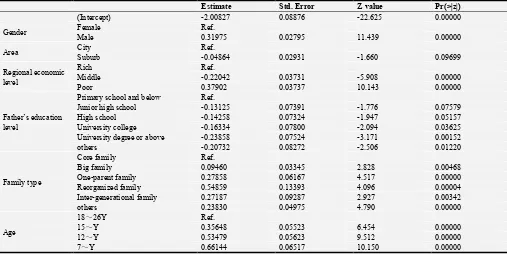
The data set K is the original complete data set, logistic regression was conducted to analyze the relationship between the variable ‘student’s injury status (yes or no) in the past one year (“Y1”) and other variables. The results of the analysis are given in Table 1. The results show that the regression coefficients of each variables are significant (P<0.05) except for the variable “Area” and “Father's educational background”, where the value of P of ‘Suburb’, ‘Junior high school’ and ‘High school’ is 0.09699 (>0.05), 0.07579 (>0.05) and 0.05157 (>0.05) respectively.
Table 1. Results of the regression analysis of complete data set K.
Estimate Std. Error Z value Pr(>|z|)
(Intercept) -2.00827 0.08876 -22.625 0.00000
Gender Female Ref.
Male 0.31975 0.02795 11.439 0.00000
Area City Ref.
Suburb -0.04864 0.02931 -1.660 0.09699
Regional economic level
Rich Ref.
Middle -0.22042 0.03731 -5.908 0.00000
Poor 0.37902 0.03737 10.143 0.00000
Father’s education level
Primary school and below Ref.
Junior high school -0.13125 0.07391 -1.776 0.07579 High school -0.14258 0.07324 -1.947 0.05157 University college -0.16334 0.07800 -2.094 0.03625 University degree or above -0.23858 0.07524 -3.171 0.00152 others -0.20732 0.08272 -2.506 0.01220
Family type
Core family Ref.
Big family 0.09460 0.03345 2.828 0.00468 One-parent family 0.27858 0.06167 4.517 0.00000 Reorganized family 0.54859 0.13393 4.096 0.00004 Inter-generational family 0.27187 0.09287 2.927 0.00342
others 0.23830 0.04975 4.790 0.00000
Age
18~26Y Ref.
15~Y 0.35648 0.05523 6.454 0.00000
12~Y 0.53479 0.05623 9.512 0.00000
3.2. Comparison Results of Thirty Complete Data Sets Processed by Three Methods
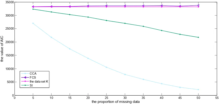
Results of thirty complete data sets are given in Figure 1. The value of AIC of 30 complete data sets processed by CCA gradually decreases from 27000 to 2100 with the increase of the proportion of missing data. Compared with the AIC of the complete data set K (33198), the relative error gradually increases. The AIC of 30 complete data sets processed by SI gradually decreases from 32000 to 21700 with the increase of the proportion of missing data. Compared with the AIC of the complete data set K, the relative error gradually increases as well. The AIC of 30 complete data sets processed by FCS
fluctuates from 33200 to 33700 with the increase of the proportion of missing data, and the relative error vary slightly. Under the similar proportion of missing data, comparing the relative error of AIC of each complete data sets processed by three methods with the result of data set K, FCS performs best and CCA performs worst. It indicated that the distribution of complete data imputed with FCS are approximately equal to the original complete real data set K. In general, with the increase of the proportion of missing data, the effect of each method gradually decreased. This indicates that the FCS is a good measure to deal with missing data compared with SI and CCA.
Figure 1. Comparison of AIC of different methods at different missing rates.
3.3. The Result of FCS
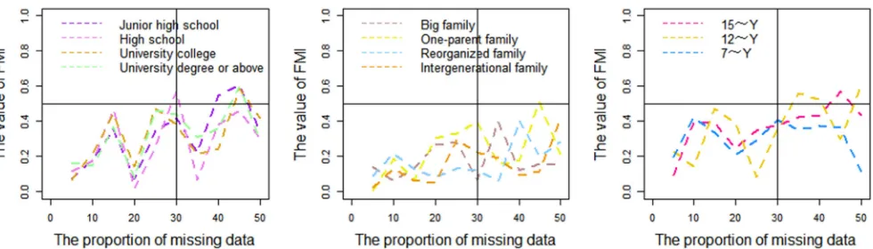
The results of logistic regression model about complete data processed by FCS at different proportion of missing data are summarized in Tables 2 and 3. It shows that for low proportion of missing data, the effect of imputation with FCS is greater, while the bias increase gradually with the increase of proportion of missing data. This result is consistent with the result in figure
1. For example, when the proportion of missing data is 10%, except for the value of β of ‘Area’ and ‘Father's education lever’, the regression coefficient of the other variables are relatively significant and the standard error of each variable is also relatively small. With the increase of proportion of missing data, especially more than 30%, values of β is meaningless in some variables, such as ‘Family typeʼ and ʻAge’.
Table 2. Results of logistic regression model about complete data processed by FCS.
5% 10% 15% 20% 25%
se Pr(>|t|) se Pr(>|t|) se Pr(>|t|) se Pr(>|t|) se Pr(>|t|)
(Intercept) 0.0921 0.0000 0.0962 0.0000 0.1031 0.0000 0.1012 0.0000 0.0984 0.0000
Gender Female Ref Ref Ref Ref Ref
Male 0.0294 0.0000 0.0291 0.0000 0.0292 0.0000 0.0315 0.0000 0.0334 0.0000 Regional
economic level
Rich Ref Ref Ref Ref Ref
Middle 0.0407 0.0000 0.0411 0.0003 0.0431 0.0008 0.0393 0.0009 0.0426 0.0073 Poor 0.0400 0.0000 0.0433 0.0000 0.0511 0.0000 0.0401 0.0000 0.0473 0.0002
Area City Ref Ref Ref Ref Ref
Suburb 0.0300 0.2223 0.0292 0.4344 0.0350 0.6674 0.0329 0.8954 0.0360 0.4557
Father’s education lever
Primary school and below Ref Ref Ref Ref Ref
Junior high school 0.0770 0.1349 0.0814 0.1942 0.0906 0.3468 0.0770 0.5161 0.0898 0.5088 High school 0.0780 0.1758 0.0801 0.1008 0.0970 0.5316 0.0744 0.3314 0.0840 0.2543 University college 0.0807 0.1214 0.0871 0.1757 0.1013 0.2660 0.0835 0.8548 0.1031 0.4413 University degree or above 0.0821 0.0052 0.0808 0.0167 0.0924 0.1357 0.0780 0.1640 0.0983 0.1308 others 0.0935 0.0548 0.0926 0.1908 0.0961 0.2952 0.0852 0.4792 0.0905 0.1652
0 5 10 15 20 25 30 35 40 45 50 55
0 5000 10000 15000 20000 25000 30000 35000
the proportion of missing data
th
e
v
a
lu
e
o
f
A
IC
5% 10% 15% 20% 25%
se Pr(>|t|) se Pr(>|t|) se Pr(>|t|) se Pr(>|t|) se Pr(>|t|)
Family type
Core family Ref Ref Ref Ref Ref
Big family 0.0384 0.0167 0.0343 0.0114 0.0358 0.0247 0.0380 0.0122 0.0384 0.0167 One-parent family 0.0735 0.0023 0.0677 0.0003 0.0645 0.0013 0.0724 0.0011 0.0735 0.0023 Reorganized family 0.1425 0.0005 0.1511 0.0023 0.1478 0.0153 0.1400 0.0011 0.1425 0.0005 Inter-generational family 0.1084 0.0230 0.1003 0.0283 0.0959 0.0100 0.0954 0.0139 0.1084 0.0230 others 0.0643 0.0197 0.0502 0.0000 0.0610 0.0010 0.0517 0.0000 0.0643 0.0197
Age
18~26Y Ref Ref Ref Ref Ref
15~Y 0.4459 0.0893 0.0661 0.0002 0.0652 0.0014 0.0583 0.0003 0.0632 0.0000 12~Y 0.6142 0.2100 0.0582 0.0000 0.0000 0.0000 0.0650 0.0000 0.0557 0.0000 7~Y 0.7602 0.1836 0.0804 0.0000 0.0745 0.0000 0.0678 0.0000 0.0724 0.0000
Table 3. Results of logistic regression model about complete data processed by FCS.
30% 35% 40% 45% 50%
se Pr(>|t|) se Pr(>|t|) se Pr(>|t|) se Pr(>|t|) se Pr(>|t|)
(Intercept) 0.1052 0.0000 0.0930 0.0000 0.1215 0.0000 0.1146 0.0000 0.1339 0.0000
Gender Female Ref Ref Ref Ref Ref
Male 0.0307 0.0000 0.0290 0.0000 0.0293 0.0000 0.0393 0.0004 0.0337 0.0004 Regional
economic level
Rich Ref Ref Ref Ref Ref
Middle 0.0409 0.0070 0.0531 0.1021 0.0458 0.1486 0.0519 0.3283 0.0549 0.2704 Poor 0.0516 0.0028 0.0478 0.0009 0.0477 0.0006 0.0719 0.0767 0.0595 0.1182
Area City Ref Ref Ref Ref Ref
Suburb 0.0333 0.5415 0.0320 0.8018 0.0307 0.8280 0.0330 0.6295 0.0404 0.5303
Father’s education level
Primary school and below Ref Ref Ref Ref Ref
Junior high school 0.0940 0.6167 0.0820 0.1001 0.1096 0.9551 0.1140 0.8494 0.0908 0.5539 High school 0.1052 0.6589 0.0747 0.0732 0.0946 0.9652 0.0986 0.9117 0.0871 0.9543 University college 0.0965 0.3336 0.0855 0.0686 0.0921 0.8804 0.1159 0.8756 0.0997 0.8083 University degree or above 0.0962 0.2454 0.0872 0.0329 0.0949 0.8440 0.1130 0.8014 0.0883 0.4260 others 0.1106 0.5993 0.0869 0.0869 0.1286 0.7680 0.1032 0.9550 0.0880 0.9177
Family type
Core family Ref Ref Ref Ref Ref
Big family 0.0341 0.0229 0.0409 0.0727 0.0351 0.0148 0.0358 0.0453 0.0356 0.2389 One-parent family 0.0772 0.0171 0.0665 0.0040 0.0681 0.0078 0.0859 0.1319 0.0698 0.1057 Reorganized family 0.1441 0.0049 0.1385 0.0033 0.1738 0.0820 0.1479 0.0021 0.1591 0.0525 Inter-generational family 0.1078 0.3050 0.1027 0.0677 0.1018 0.4282 0.1001 0.0746 0.1201 0.3776 others 0.0594 0.0221 0.0582 0.0502 0.0523 0.0134 0.0649 0.0445 0.0587 0.1354
Age
18~26Y Ref Ref Ref Ref Ref
15~Y 0.0625 0.0193 0.0636 0.0223 0.0642 0.0214 0.0708 0.0799 0.0632 0.1053 12~Y 0.0630 0.0002 0.0728 0.0051 0.0708 0.0067 0.0594 0.0015 0.0758 0.1019 7~Y 0.0763 0.0003 0.0728 0.0001 0.0745 0.0102 0.0726 0.0034 0.0626 0.0078
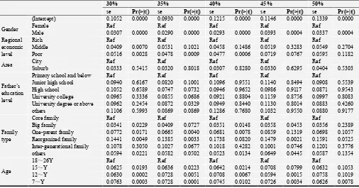
The results in the Figure 2 show that the values of FMI of different variables at different proportion of missing data. It indicates that the value of FMI of a certain variable will increase with the proportion of missing data. For example, the FMI of ‘Poor region’ and ‘15~Y’ changes from approximately 0.1 to 0.7 and 0.1 to 0.6, respectively, as the proportion of missing data become high. It reflects that the variability
Figure 2. The FMI of different variables at different proportion of missing data.
4. Discussion
Under MCAR, the effects of three methods processing survey data with missing value at different missing rates are analyzed. The results show that FCS perform well compared with CCA and SI, which are consistent with other papers [2-3]. Under MCAR, The result of AIC shows substantial differences between in CCA and original data set K, the higher percentage of missing data, the more significant difference of the relative error of AIC. Because of its simple operation, CCA has become the most commonly used method to process missing data in scientific research. However, this method often results in bias because of potential loss of information [2, 11]. So it suggests that deleting the sample with missing value directly should be avoided. Alternatively, SI based on substituting the missing values with mode can maximally retains the integrity of the data. However, the approach may result in potential loss of the distributional relationship among variables and it is not possible to provide measures of uncertainty introduced by the imputation process. When the proportion of missing data is low (such as 5%), the processing performs better. And when more missing information appears, it will lead to the variance of the estimated parameters to be biased. In our study, we found MI is the preferred method for dealing with missing data, and in both simulation research and practical applications it showed good ability to process missing data [1, 10-11, 25]. The observed data was preserved and the imputation data was concerned as well in MI. Hence, FCS was utilized to estimate missing values and obtain unbiased estimates. This study uses FCS because it does not require stricter model assumptions as multivariate normal (MVN) [26], and it is a very flexible method to deal with missing data as long as the imputation model is correctly specified [10, 27].
The value of FMI can also be used as an indicator to guide the application of MI [17]. The FMI contains the fraction of the missing information as defined in Rubin [13], that is, the proportion of the overall uncertainty due to the missing data. The statistic of FMI is as small as possible. When the proportion of missing data is low, the value of FMI is small which indicates that the imputation result of MI is effective. As the proportion of missing data gradually increase, the value of FMI gradually increase and the effect of imputation
gradually becomes worse. An explanation to this is that the more data is missing, the less usable the data set and the information it reflects. So the change of FMI reflects the effective of MI to process missing value.
Researchers in a variety of fields often concern what is the proper scope of application for MI in terms of the proportion of missing data [23]. In this paper we found 30% is the scope of MI. Because when the proportion of missing data less than 30%, the imputed effect of FCS is relatively stable. For example, when the missing data rate is 10%, except for the β of “Area” and “Father's education lever”, that of other variables are relatively significant and the standard error is small. It indicates that both the deviation and the mean square error between FCS and the original data set K are small and the model results obtained by FCS are consistent with the original model results. When it is more than 30%, the β of variables becomes meaningless and variables with a value of FMI increasing 0.5 or above becomes more. Although some studies suggested that MI can achieve a good imputed effect when the proportion of missing data is 40% or even 90% [23], the bias of variables become increasing with the increase of proportion of missing data, which was another discovery in our study.
Compared with prior studies, our study has two advantages. First, more complex data structures were used and more variables were tested including multivariate variables [5-6, 23]. Our simulation study is a multivariate missing data set, including binary, unordered and ordered categorical variables, which is closer to the actual situation of missing data in the survey data compared with the single variable missing pattern [17]. Second, more methods were concerned together such as MI, CCA and SI [1, 10, 23], which makes the results more reliable.
gradually decreases [23, 30]. In this study, large sample data were used, and compared with small sample size, the results have better influence efficiency.
However, this study also has some shortcomings. We only studied the processing method under the mechanism of MCAR, and does not study the scenario under MNAR. In practical research, we need to figure out the missing mechanism of data set and then conduct sensitivity analysis [11, 31]. That's what we're trying to do and we hope more scholars to study it in the future.
5. Conclusions
Missing data is a pervasive problem that should be dealt with appropriately. In this paper, the performance of three methods that processing incomplete data under MCAR was evaluated. Under different proportion of missing data, the MI performs well compared with CCA and SI. Second, the changing of FMI can also be used as an indicator of MI to process missing data. Third, it is suitable for MI to process large sample data, and no more than 30% of proportion of missing data is the proper scope of application of MI. It is expected to provide a methodological reference for the similar survey data to process missing values, and solve the problem of inspection efficiency reducing caused by data loss, and provide experience for researchers.
References
[1] Chinomona A, Mwambi H. Multiple imputation for non-response when estimating HIV prevalence using survey data. BMC Public Health, 2015, 15 (1): 1059.
[2] Harel O, Mitchell E M, Perkins N J, et al. Multiple Imputation for Incomplete Data in Epidemiologic Studies. American Journal of Epidemiology, 2017.
[3] Ma Y, Zhang W, Lyman S, et al. The HCUP SID Imputation Project: Improving Statistical Inferences for Health Disparities Research by Imputing Missing Race Data. Health Services Research, 2017.
[4] Hughes RA, Heron J, Sterne JAC, Tilling K. Accounting for missing data in statistical analyses: multiple imputation is not always the answer. International Journal of Epidemiology, 2019.
[5] Mukaka M, White S A, Terlouw D J, et al. Is using multiple imputation better than complete case analysis for estimating a prevalence (risk) difference in randomized controlled trials when binary outcome observations are missing?. Trials, 2016, 17 (1): 341.
[6] Alma P, Ellen M, Deirdre C F, et al. Missing data and multiple imputation in clinical epidemiological research. Clinical Epidemiology, 2017, Volume 9: 157-166.
[7] Sullivan D, Andridge R. A hot deck imputation procedure for multiply imputing nonignorable missing data: The proxy pattern-mixture hot deck. Computational Statistics & Data Analysis, 2015, 82: 173-185.
[8] Rodwell L, Lee K J, Romaniuk H, et al. Comparison of
methods for imputing limited-range variables: a simulation study. BMC Medical Research Methodology, 2014, 14 (1): 57. [9] Allotey P A, Harel O. Multiple Imputation for Incomplete Data in Environmental Epidemiology Research. Current Environmental Health Reports, 2019.
[10] Liu Y, De A. Multiple Imputation by Fully Conditional Specification for Dealing with Missing Data in a Large Epidemiologic Study. International Journal of Statistics in Medical Research, 2015, 4 (3): 287-295.
[11] Hayati Rezvan P, Lee K J, Simpson J A. The rise of multiple imputation: a review of the reporting and implementation of the method in medical research. BMC Medical Research Methodology, 2015, 15 (1): 30.
[12] Mackinnon A. The use and reporting of multiple imputation in medical research - a review. Journal of Internal Medicine, 2010, 268 (6): 586-593.
[13] Buuren S v, Groothuis-Oudshoorn K. mice: Multivariate Imputation by Chained Equations in R. Journal of Statistical Software, Articles, 2011, 45 (3): 1-67.
[14] Azur M J, Stuart E A, Frangakis C, et al. Multiple imputation by chained equations: what is it and how does it work?. International Journal of Methods in Psychiatric Research, 2011, 20 (1): 40-49.
[15] Enders C K, Keller B T, Levy R. A Fully Conditional Specification Approach to Multilevel Imputation of Categorical and Continuous Variables. Psychological Methods, 2017. [16] Harel O, Zhou X H. Multiple imputation: review of theory,
implementation and software. Statistics in medicine, 2007, 26 (16): 3057-3077.
[17] Zhang Z. Multiple imputation with multivariate imputation by chained equation (MICE) package. Ann Transl Med, 2016, 4 (2): 30.
[18] Honaker J, King G, Blackwell M. Amelia II: A program for missing data. Journal of statistical software, 2012, 45 (7): 1-47. [19] Ayilara OF, Zhang L, Sajobi TT, Sawatzky R, Bohm E, Lix LM.
Impact of missing data on bias and precision when estimating change in patient-reported outcomes from a clinical registry. Health and Quality of Life Outcomes, 2019, 17 (1): 106. [20] Sun B L, Perkins N J, Cole S R, et al.
Inverse-Probability-Weighted Estimation for Monotone and Nonmonotone Missing Data. American Journal of Epidemiology, 2017.
[21] Seaman S R, White I R. Review of inverse probability weighting for dealing with missing data. Statistical Methods in Medical Research, 2013, 22 (3): 278.
[22] Bartlett J W, Carpenter J R, Tilling K, et al. Improving upon the efficiency of complete case analysis when covariates are MNAR. Biostatistics, 2014, 15 (4): 719-730.
[23] Madley-Dowd P, Hughes R, Tilling K, Heron J. The proportion of missing data should not be used to guide decisions on multiple imputation. Journal of Clinical Epidemiology, 2019, 110: 63-73.
[25] Waljee A K, Mukherjee A, Singal A G, et al. Comparison of imputation methods for missing laboratory data in medicine. BMJ Open, 2013, 3 (8): e002847-e002847.
[26] Lee K J, Carlin J B. Multiple Imputation for Missing Data: Fully Conditional Specification Versus Multivariate Normal Imputation. American Journal of Epidemiology, 2010, 171 (5): 624-632.
[27] White I R, Carlin J B. Bias and efficiency of multiple imputation compared with complete-case analysis for missing covariate values. Statistics in medicine, 2010, 29 (28): 2920-2931.
[28] Greenland S, Finkle W D. A critical look at methods for handling missing covariates in epidemiologic regression
analyses. American Journal of Epidemiology, 1995, 142 (12): 1255-1264.
[29] Hardt J, Herke M, Leonhart R. Auxiliary variables in multiple imputation in regression with missing X: a warning against including too many in small sample research. BMC Medical Research Methodology, 2012, 12 (1): 184.
[30] Hardt J, Herke M, Brian T, Laubach W. Multiple imputation of missing data: a simulation study on a binary response. Open J Stat, 2013; 3 (05): 370.