Analysis on ECG Data Compression Using Wavelet Transform Technique

(1)

http://www.sciencepublishinggroup.com/j/ijpbs doi: 10.11648/j.ijpbs.20170206.12

ISSN: 2575-2227 (Print); ISSN: 2575-1573 (Online)

Analysis on ECG Data Compression Using Wavelet

Transform Technique

Hla Myo Tun

1

, Win Khaing Moe

2

, Zaw Min Naing

2

1_{Department of Electronic Engineering, Yangon Technological University, Yangon, Myanmar} 2

Department of Research and Innovation, Ministry of Education, Yangon, Myanmar

Email address:

[email protected] (H. M. Tun), [email protected] (W. K. Moe), [email protected] (Z. M. Naing)

To cite this article:

Hla Myo Tun, Win Khaing Moe, Zaw Min Naing. Analysis on ECG Data Compression Using Wavelet Transform Technique. International Journal of Psychological and Brain Sciences. Vol. 2, No. 6, 2017, pp. 127-140. doi: 10.11648/j.ijpbs.20170206.12

Received: October 8, 2017; Accepted: October 18, 2017; Published: December 22, 2017

Abstract:

Although digital storage media is not expensive and computational power has exponentially increased in past few years, the possibility of electrocardiogram (ECG) compression still attracts the attention, due to the huge amount of data that has to be stored and transmitted. ECG compression methods can be classified into two categories; direct method and transform method. A wide range of compression techniques were based on different transformation techniques. In this work, transform based signal compression is proposed. This method is used to exploit the redundancy in the signal. Wavelet based compression is evaluated to find an optimal compression strategy for ECG data compression. The algorithm for the one-dimensional case is modified and it is applied to compress ECG data. A wavelet ECG data code based on Run-length encoding compression algorithm is proposed in this research. Wavelet based compression algorithms for one-dimensional signals are presented along with the results of compression ECG data. Firstly, ECG signals are decomposed by discrete wavelet transform (DWT). The decomposed signals are compressed using thresholding and run-length encoding. Global and local thresholding are employed in the research. Different types of wavelets such as daubechies, haar, coiflets and symlets are applied for decomposition. Finally the compressed signal is reconstructed. Different types of wavelets are applied and their performances are evaluated in terms of compression ratio (CR), percent root mean square difference (PRD). Compression using HAAR wavelet and local thresholding are found to be optimal in terms of compression ratio.

Keywords:

ECG, Compression Technique, Wavelet Transform Technique, Biomedical Engineering, Signal Processing, Biomedical Science

1. Introduction

Compression/coding of Electrocardiogram (ECG) signal are done by detecting and removing redundant information from the ECG signal [1]. ECG data compression algorithm is either of two categories. One method is direct data compression method [2], which detects redundancies by direct analysis of actual signal samples. Another method is transform method, which first transforms the signal to some other time–frequency representations better suited for detecting and removing redundancies. Among transform methods, the wavelet transform method has been shown promise because of their good localization properties in the time and frequency domain.

The purpose of ECG compression is to reduce the amount

of bits needed to transmit and to store digitized ECG data as much as possible with a reasonable implementation of complexity while maintaining clinically acceptable signal quality. However, serious difficulties are encountered in attempting to reduce the channel costs and electronic resources. Several attempts have been made which partly solve the problem using compression algorithms [3]. The performance improvements of the conventional compression algorithms are required for the continuous acquisition of electrocardiogram (ECG). The main goal of an optimized compression technique is to minimize the number of samples needed to transmit the ECG without losing the remarkable information of the original signal in order to achieve a correct clinical diagnosis.

(2)

of sub-band and wavelet based methods in signal processing, much work has been done in ECG compression using these techniques [2]. There are a great number of wavelet compression techniques available in the literature. However, the search for new methods and algorithms continues to achieve higher compression ratio while preserving the clinical information content in the reconstructed signal. Naturally, the clinical acceptability of the reconstructed signal depends on the intended data application and the common way to measure it through visual inspection. The use of the percent root mean square difference (PRD) has become common practice to the scientific community as a measure of fidelity of any ECG compression algorithm. Weighted diagnostic distortion (WDD) measure is another method recently being investigated although it needs the subjective test by expert physiologists.

Recently developed wavelet transforms have become an attractive and efficient tool in many applications especially in coding and compression of signals. This results from their multi-resolution and high-energy compaction properties. Wavelet transform can be viewed as a block transform with overlapping basis functions of variable lengths. Since WT

results large runs or zeros in the transformed signal, it can be efficiently used for compression. Moreover, the nonzero small coefficients can be thresholded using appropriate techniques with a further increase in the number of zeros. Hence, improvement in the compression ratio is expected. In technical literature there exist a large number of thresholding techniques. Among them the universal thresholding [4], and thresholding methods based on energy packing efficiency [5] are the most efficient methods. In the process of thresholding, there is the need of compromise between compression ratio and the quality of the reconstructed signal [6].

2. System Description

In this work, the wavelet transform methods are used for the signal compression. For ECG compression, three most commonly used steps are DWT decomposition, thresholding and run-length encoding. A compressed signal and its reconstructed signal form are obtained from described methodology. A typical block diagram of the methodology is depicted in Figure 1.

Figure 1. Overall Block Diagram of the ECG Signal Compression.

3. Optimization Methods for ECG

Compression

More recently, many interesting optimization based ECG compression methods, the third category, have been developed. The goal of most of these methods is to minimize the reconstruction error given a bound on the number of samples to be extracted or the quality of the reconstructed signal to be achieved. In [4], the goal is to minimize the reconstruction error given a bound on the number of samples to be extracted. The ECG signal is compressed by extracting the signal samples that, after interpolation, will best represent the original signal given an upper bound on their number. After the samples are extracted they are Huffman encoded. This leads to the best possible representation in terms of the

number of extracted signal samples, but not necessarily in terms of bits used to encode such samples. The bit rate has been taken into consideration in the optimization process.

The vast majority of the above mentioned methods do not permit perfect reconstruction of the original signals. In fact; there is no automatic way to assure that the distortion in the reconstructed signal will not affect clinically important features of the ECG. To preserve the clinical diagnostic features of the reconstructed ECG signals both the wavelet filters’ parameters and the threshold levels in all subbands should be selected carefully. Thus, the aim is to present ECG compression technique that achieves maximum data volume reduction while preserving the significant signal morphology features upon reconstruction.

(3)

through parameterization of the wavelet filters and the selection of optimum threshold levels of the wavelet coefficients in different subbands [7].

4. Techniques of Data Compression

There are three important techniques of data compression.

Basic technique Statistical technique Dictionary technique

4.1. Basic Technique

These are the techniques, which have been used only in the past. The important basic techniques are run length encoding and move to front encoding.

4.2. Run-Length Encoding

Run-length encoding is a data compression algorithm that is supported by most bitmap file formats, such as TIFF, BMP, and PCX. RLE is suited for compressing any type of data regardless of its information content, but the content of the data will affect the compression ratio achieved by RLE. Although most RLE algorithms cannot achieve the high compression ratios of the more advanced compression methods, RLE is both easy to implement and quick to execute, making it a good alternative to either using a complex compression algorithm or leaving your image data uncompressed.

RLE works by reducing the physical size of a repeating string of characters. This repeating string, called a run, is typically encoded into two bytes. The first byte represents the number of characters in the run and is called the run count. In practice, an encoded run may contain 1 to 128 or 256 characters; the run count usually contains as the number of characters minus one (a value in the range of 0 to 127 or 255). The second byte is the value of the character in the run, which is in the range of 0 to 255, and is called the run value.

The basic idea behind this approach to data compression is this: if a data item occurs n consecutive times in the input stream replace the n occurrences with a single pair <n d>. The n consecutive occurrences of a data item are called run length of n and this approach is called run length encoding or RLE [8].

4.3. RLE Image Compression

RLE is a natural candidate for compressing graphical data. A digital image consists of small dots called pixels. Each pixel can be either one bit indicating a black or white dot or several bits indicating one of several colors or shades of gray. We assume that these pixels are stored in an array called bitmap in the memory. Pixels are normally arranged in the bit map in scan lines. So the first bit map pixel is the dot at the top left corner of the image and the last pixel is the one at the bottom right corner. Compressing an image using RLE is based on the observation that if we select a pixel in the image at random there is a good chance that its neighbors will have

the same color. The compressor thus scans the bit map row by row looking for runs of pixels of same color.

Consider the grayscale bitmap-

12, 12, 12, 12, 12, 12, 12, 12, 12, 35, 76, 112, 67, 87, 87, 87, 5, 5, 5, 5, 5, 5, 1- - -

Compressed Form-

9, 12, 35, 76, 112, 67, 3, 87, 6, 5, 1- - -

4.4. Move to Font Coding

The basic idea of this method is to maintain the alphabet A of symbols as a list where frequently occurring symbols are located near the front. A symbol 'a' is encoded as the no of symbols that precede it in this list. Thus if A= ('t', 'h', 'e', 's') and the next symbol in the input stream to be encoded is 'e', it will be encoded as '2' since it is preceded by two symbols. The next step is that after encoding 'e' the alphabet is modified to A= ('e', 't', 'h', 's'). This move to front step reflects the hope that once 'e' has been read from the input stream it will read many more times and will at least for a while be a common symbol.

Let A= (t, h, e, s)

After encoding the symbol e, A is modified. Modified Form-

A= (e, t, h, s)

4.5. Advantages

This method is locally adaptive since it adapts itself to the frequencies of the symbol in the local areas of input stream. This method produces good results if the input stream satisfies this hope that is if the local frequency of symbols changes significantly from area to area in the input stream [7].

4.6. Statistical Technique

They are based on the statistical model of the data. Under this statistical technique there come three important techniques

Shannon Fano coding Huffman coding Arithmetic coding

4.7. Shannon Fano Coding

(4)

The two symbols in the first subset are assigned codes that start with 1, so their final codes are 11 and 10. The second subset is divided in the second step, into two symbols and three symbols. Step 3 divides last three symbols into 1 and 2.

4.8. Huffman Coding

A commonly used method for data compression is Huffman coding. The method starts by building a list of all the alphabet symbols in descending order of their probabilities. It then constructs a tree with a symbol at every leaf from the bottom up. This is done in steps where at each step the two symbols with smallest probabilities are selected, added to the top of partial tree, deleted from the list and replaced with an auxiliary symbol representing both of them. When the list is reduced to just one auxiliary symbol the tree is complete. The tree is then traversed to determine the codes of the symbols. The Huffman method is somewhat similar to Shannon fano method. The main difference between the two methods is that Shannon fano constructs its codes from top to bottom while Huffman constructs a code tree from bottom up. This is best illustrated by an example. They are paired in the following order:

a4 is combined with a5 and both are replaced by the combined symbol a45, Whose probability is 0.2.

There are now four symbols left, a1, with probability 0.4, and a2, a3, and a45, with probabilities 0.2 each. It is arbitrarily selected a3 and a45 combine them and replace them with the auxiliary symbol a345, whose probability is 0.4.

Three symbols are now left, a1, a2, and a345, with probabilities 0.4, 0.2, and 0.4 respectively. a2 and a345 are arbitrarily selected, combine them and replace them with the auxiliary symbol a2345, whose probability is 0.6.

Finally, the two remaining symbols a1, and a2345 are combined, and replace them with a12345 with probability 1. The tree is now complete, lying on its side with the root on the right and the five leaves on the left. To assign the codes, we arbitrarily assign a bit of 1 to the top edge, and a bit of 0 to the bottom edge of every pair of edges. This results in the codes 0, 10, 111, 1101, and 1100. The assignments of bits to the edges are arbitrary.

The average size of this code is 0.4 x 1 + 0.2 x 2 + 0.2 x 3 + 0.1 x 4 + 0.1 x 4 = 2.2 bits / symbol, but even more importantly, the Huffman code is not unique [7].

4.9. Arithmetic Coding

In this method the input stream is read symbol by symbol and appends more to the code each time a symbol is input and processed. To understand this method it is useful to imagine the resulting code as a number in the range [0, 1) that is the range of real numbers from 0 to 1 not including one.

The first step is to calculate or at least to estimate the frequency of occurrence of each symbol. The foresaid techniques that is the Huffman and the Shannon Fano techniques rarely produce the best variable size code. The arithmetic coding overcomes this problem by assigning one

code to the entire input stream instead of assigning codes to the individual bits.

The main steps of arithmetic coding are

Start by defining the current interval as [0, 1]

Repeat the following two steps for each symbol’s’ in the input stream.

Divide the current interval into subintervals whose sizes are proportional to the probability of the symbol.

Select the sub interval for’s’ and define it as the new current interval.

When the entire input stream has been processed in this way the output should be any number that uniquely identifies the current interval.

Consider the symbols a1, a2, a3

Probabilities â€∞ P1= 0.4. P2=0.5, P3=0.1 Subintervals â€∞ [0-0.4] [0.4-0.9] [0.9-1] To encode â€∞ a2 a2 a2 a3

Current interval â€∞ [0, 1] a2 [0.4-0.9]

a2 [0.6-0.85] {0.4 + (0.9-0.4)0.4 = 0.6} {0.4 + (0.9-0.4)0.9 = 0.85}

a2 [0.7-0.825] {0.6 + (0.85-0.6)0.6 = 0.7} {0.6 + (0.85-0.6)0.85 = 0.825}

a3 [0.8125-0,8250] {0.7 + (0.825-0.7)0.7 = 0.8125} {0.7 + (0.825-0.7)0.825 =0.8250}

Dictionary Technique

This method select strings of symbols and encodes each string as a token using a dictionary. The important dictionary methods are

LZ77 (sliding window) and LZRW1

4.10. LZ77 (Sliding Window)

The main idea of this method is to use part of previously seen input stream as the dictionary. The encoder maintains a window to the input stream and shifts the input in that window from right to left as strings of symbols are being encoded. The method is thus based on "sliding window". The window is divided into two parts that is search buffer, which is the current dictionary and lookahead buffer, containing text yet to be encoded [7].

4.11. LZRW1 Technique

The main idea is to find a match in one step using a hash table. The method uses the entire available memory as a buffer and encodes the input string in blocks. A block is read into the buffer and is completely encoded. Then the next block is read and encoded and so on. These two buffers slide along the input block in memory from left to right. It is necessary to maintain only one pointer pointing to the start of look ahead buffer.

(5)

p points outside the search buffer there is no match, the first character in the look ahead buffer is output as literal and pointer is advanced by one. The same thing is done if p points outside the search buffer but to a string that does not match with the one in look ahead buffer. If p points to a match of at least three characters the encoder finds the longest match, outputs a match item and advances the pointer by the length of the match [7].

5. Performance Measures for

Compression Algorithms

There are two types of judgment for compression performance measurement. They are

Subjective judgment and Objective judgment

5.1. Subjective Judgment

The most obvious way to determine the preservation of diagnostic information is to subject the reconstructed data for evaluation by a cardiologist. This approach might be accurate in some cases but suffers from many disadvantages. One drawback is that it is a subjective measure of the quality of reconstructed data and depends on the cardiologist being consulted, thus different results may be presented. Another shortcoming of the approach is that it is highly inefficient. Moreover, the subjective judgment solution is expensive and can generally be applied only for research purposes [8].

5.2. Objective Judgment

Compression algorithms all aim at removing redundancy within data, thereby discarding irrelevant information. In the case of ECG compression, data that does not contain diagnostic information can be removed without any loss to the physician. To be able to compare different compression algorithms, it is imperative that an error criterion is defined such that it will measure the ability of the reconstructed signal to preserve the relevant diagnostic information. The criteria for testing the performance of the compression algorithms consist of three components: compression measure, reconstruction error and computational complexity. The compression measure and the reconstruction error depend usually on each other and determine the rate-distortion function of the algorithm. The computational complexity component is related to practical implementation consideration and is desired to be as low as possible [8].

6. Performance Evaluation of

Compression

Several techniques exist for evaluating the quality of compression algorithms.

The performance of the wavelet filters in the field of ECG signal compression can be

evaluated by considering the fidelity of the reconstructed

signal to the original signal. For this, following fidelity assessment parameters are considered:

Compression ratio (CR) Root Mean Square Error (RMS)

Percent Root-mean-square Difference (PRD) Signal to Noise Ratio (SNR)

6.1. Compression Ratio (CR)

The compression ratio (CR) is defined as the ratio of the number of bits representing the original signal to the number required for representing the compressed signal. So, it can be calculated from:

Compression Ratio = P B

C

×

(1)

Where,

P = Number of ECG samples, B = Bit depth per sample and C = Compressed ECG file size

Another way for calculating the compression ratio is as follow:

Number of significant encoded wavelet coefficients CR

Total number of coefficients

= (2)

6.2. Root Mean Square Error (RMS)

In some literature, the root mean square error (RMS) is used as an error estimate. The RMS is defined as

(

)

N

2

n 1

ˆ x(n) x(n) RMS

N

=

− =

∑

₍₃₎

where x (n) is the original signal, x̂ (n) is the reconstructed signal and N is the length of the window over which the RMS is calculated [9]. This is a purely mathematical error estimate without any diagnostic considerations.

6.3. Percent Root-Mean-Square Difference (PRD)

(6)

(

)

N 2 n 1 N 2 n 1 ˆ x(n) x(n) PRD x (n) = = − =

∑

(4)

This error estimate is the one most commonly used in all scientific literature concerned with ECG compression techniques. The main drawbacks are the inability to cope with baseline fluctuations and the inability to discriminate between the diagnostic portions of an ECG curve. However, its simplicity and relative accuracy make it a popular error estimate among researchers [1].

6.4. Signal to Noise Ratio (SNR)

Basically signal to noise ratio (SNR) is an engineering term for the power ratio between a signal and noise. It is expressed in terms of the logarithmic decibel scale.

2 Esignal SNR _{10 log10}

Enoise     = _ _   (5) Esignal SNR _{20 log10}

Enoise     = _ _   (6)

In some literature, the signal to noise ratio (SNR) is also used as an error estimate. The SNR is defined as

2 2 x (n) SNR x(n) y(n)     =  −    

∑

(7)

x (n) is the original 1-D signal and y (n) is the reconstructed signal [11].

6.5. Methodology for Signal Compression

In this work, the wavelet transform methods are used for the signal compression. For ECG compression, three most commonly used steps are DWT decomposition, thresholding and run-length encoding. A compressed signal and its reconstructed signal form are obtained from described methodology. Here, compression methodology can be illustrated in following three steps:

Step I. In this step, the mother wavelet is chosen, and then DWT decomposition is performed on the speech and ECG signal. Several different criteria can be used for selecting the optimal wavelet filter. For example, the optimal wavelet filter must minimize the reconstructed error variance and also maximize signal to noise ratio (SNR). In general, the mother wavelets are selected based on the energy conservation properties in the approximation part of the wavelet coefficients. Then, decomposition level for DWT is selected which usually depends on the type of signal being analyzed. Here, the beta wavelets are used as the mother wavelet and

different decomposition level of DWT is applied on the ECG signal.

Step II. After computing the wavelet transform of the 1-D signal, compression involves truncating wavelet coefficients below a threshold which make a fixed percentage of coefficients equal to zero. The Global thresholding involves taking the wavelet decomposition of the signal and keeping the largest absolute value coefficients. In this, the threshold value is set manually and this value is chosen from DWT coefficient (0…. xmaxj), where xmaxjis the maximum value of

coefficient.

Step III. In this step, signal compression is further achieved by efficiently encoding the truncated small valued coefficients. The resulting signal data contains same redundant data which is waste of space. In this work, Run-length encoding is applied on the redundant data for overcoming the redundancy problem without any loss of signal data. Run -length coding is a simple form of data compression in which run of data are stored as a single data value and count, rather than as the original run. Finally, the encoded compressed data are decoded and reconstructed to get the original signal.

6.6. Algorithm

The ECG signal compression algorithm is developed as following steps:

BEGIN

Load signal (MIT-BIH Database)

Transform the original signal using by discrete wavelet transform (DWT)

Find the maximum value of the transformed coefficients and apply a fix percentage based hard threshold.

Run-length encoding applied on the coefficients without any loss of signal data.

Apply Run-length decoding

Apply inverse transform to get the reconstruct signal Calculate Percent Root Mean Square Difference (PRD) Calculate Compression Ratio (CR).

Display the result END

7. Loading ECG Signal

To make results independent of the features of a speciﬁed ECG waveform, five types of ECG signals were tested with different features including a 10-min record (3600 samples) taken from the MIT-BIH Arrhythmia Database Record 200 sampled at 360 Hz with 11-bit resolution, an a trial ﬁbrillation record, an angina pectoris record and a normal ECG record.

7.1. MIT-BIH Arrhythmias Database

(7)

There are 116,137 numbers of QRS complexes in the database [6]. The subjects were taken from, 25 men aged 32 to 89 years, and 22 women aged 23 to 89 years and the records 201 and 202 came from the same male subject. Each recording includes two leads; the modified limb lead II and one of the modified leads V1, V2, V4 or V5. Continuous ECG signals are band pass-filtered at 0.1–100 Hz and then digitized at 360 Hz. Twenty-three of the recordings (numbered in the range of 100–124) are intended to serve as a representative sample of routine clinical recordings and 25 recordings (numbered in the range of 200–234) contain complex ventricular, junctional, and supraventricular arrhythmias. The database contains annotation for both timing information and beat class information verified by independent experts [8].

7.2. Compression Algorithms

ECG signal compression using wavelet transform is performed with following steps [13-17]:

Read ECG samples from the MIT Database. Each signal consists of 3600 samples.

Apply wavelet transform on the signal of 3600 samples. Apply thresholding (replace small wavelet coefficients by zero).

Encode wavelet coefficients by run length encoding method

ECG signal is reconstructed using inverse wavelet transform with following steps:

Read the wavelet coefficients from the compressed file. Decode wavelet coefficients by run length decoding. (Restore zeros).

Apply inverse wavelet transform on the signal. Reconstructed the ECG signal

7.3. Wavelet Transform Algorithms

The wavelet transform algorithms using Haar, Daubechies series wavelet used in this research are presented here [18-22].

7.3.1. Haar Wavelet Transform Algorithm

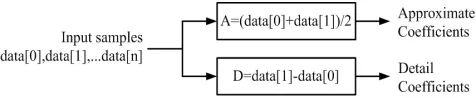
Let us consider a sequence of data samples: data [0], data [1],…….., data [n].

Haar transform on this sequence can be calculated with following steps:

The sequence of data samples is divided into two frames: odd frame and even frame.

Samples of odd frame are subtracted from samples of even frame that gives detail coefficients.

Even samples are replaced by average of even and odd samples that gives average coefficients.

Figure 2. Haar Wavelet Decomposition Structure.

Harr wavelet decomposition structure is shown in Figure 2. The approximate coefficients “A” and detail coefficients “D”

are overwritten on the same data sequence to save memory: data [1] = D or data [1] = data [1] – data [0]

data [0] = A or data [0] = data [0] + data [1]/2

Inverse Haar transform can be calculated by changing the sign of operation.

data [0] = data [0]-data [1]/2 data [1] = data [1] + data [0]

7.3.2. Daubechies Wavelet Transforms

Daubechies wavelets are very popular because they are good compromise between compact support and smoothness.

In the filter bank implementation, ECG samples f (k) are applied at the input of Daubechies wavelet filter bank. The input ECG samples are convolved with low-pass and high-pass analysis filters h and g. The output of each filter is down-sampled by two, yielding the transformed signals cA0 and cD0. Down-sampling is performed to keep total number of transformed coefficients same as that of input samples.

The coarse information cA0 is further applied at the input of analysis filter bank and decomposed into cA1 and cD1. This process is repeated “N” times to achieve “N level” decomposition.

Equation 8 and 9 describes practical implementation of Daubechies wavelet transform. This implementation is fast compare to pyramidal algorithm in which wavelet filter coefficients are arranged in form of matrix and matrix is multiplied with input samples. In pyramidal algorithm, half of the computation is waste because of down sampling [23-27].

N 1

j

m 0

cA (k) h(m)f(m 2k)

−

=

∑

+ (8)

N 1

j

m 0

cD (k) g(m)f(m 2k)

−

=

∑

+ (9)

Where, cAj (k) =Coarse coefficients at level j cDj (k) = Detail coefficients at level j h (m) = Low pass filter coefficients g (m) = High pass filter coefficients N= Number of filter coefficients

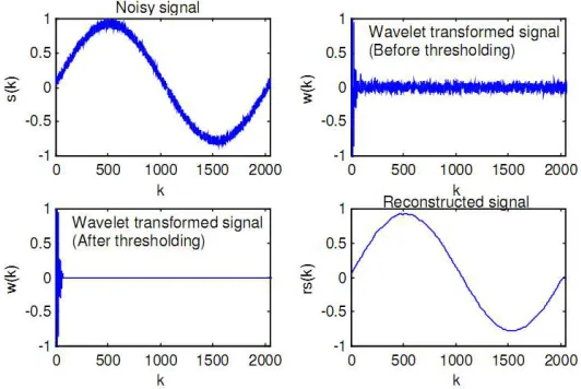
7.3.3. De-Noising by Thresholding

Thresholding process not only gives compression but also removes noise from the signal. The wavelet coefficients close to zero contains little information and it is influenced by noise.

Let us consider the signal s (k) corrupted with noise h:

n

S (k)=S(k) h+ (10)

When wavelet transform is applied on noisy signal Sn (k),

(8)

Figure 3. Noise Removal with Threshold.

There are two methods proposed by the Donoho for the removal of the noise from the signal.

Hard thresholding: In hard thresholding, all the coefficients below the threshold value are set to zero and other coefficients are not affected. Thus it is a “keep-or-kill” procedure.

w(k)=w(k), w(k) Th

0, w(k) Th >

= ≤ (11)

Soft thresholding: In soft thresholding, all the coefficients below the threshold value are set to zero and remaining coefficients are shrunken. The amount of shrinking is equal to threshold value.

w(k)=sgn(w(k)), ( w(k) Th), w(k) Th

0, w(k) Th

− >

= ≤ (12)

7.4. Encoding Methods

The number of zeros and small wavelet coefficients are obtained after applying wavelet transform on the ECG signal. If small wavelet coefficients are replaced with zeros by applying thresholding, number of zeros will increase. If the wavelet coefficients are stored after thresholding, any compression will not be achieved because storage of zeros will also require memory space.

Advantage of applying wavelet transform for the ECG compression becomes evident if encoding is applied to take advantage of series of zeros present in the sequence. If encoding is directly applied on the speech samples, much compression will not be achieved.

Wavelet transform gives sparse organized data with sequence of zeros, hence encoding after the wavelet transform gives good compression. Hence some encoding methods are necessary to take advantage of wavelet transform for the speech compression.

Encoder allocates less number of bits to the zeros. To encode the wavelet-transformed ECG signal, run-length encoding method is used in this work. Run-length encoding

is very attractive from the point of view of the ECG compression. All the results presented in this study are based on run-length encoding after wavelet transform.

8. Flowchart of the ECG Signal

Compression

Flowchart of the ECG signal compression is shown in Figure 4.

(9)

The ECG signal compression algorithm is developed in MATLAB environment. Firstly ECG signal from MIT-BIH database is loaded into the MATLAB workspace. Then, the signal is decomposed by choosing level (multi or single) and defining wavelet name (“db” or “Haar”). The coefficients which are obtained from decomposition are de-noised and compressed by thresholidng. And then, run-length encoding method is applied. Compressed ECG signal is obtained from this step. The encoded signal is decoded. Finally the signal is reconstructed by inverse wavelet transform. The quality of compression algorithm is tested by calculating compression ratio (CR) and Percent Root-mean-square Difference (PRD).

9. Experimental Results

The experimental data from MIT/BIH arrhythmia database is used to analyze and test the performance of coding scheme. Various ECG signal records are used for experiments and algorithm is tested for 3600 samples from each record 100, 101, 102, 105, 110, 113, 117, 119, 205, 209 and 210. The database is sampled at 360Hz and the resolution of each sample is 11 bits/sample.

In this section, MATLAB program is applied on a set of ECG signals in order to investigate the performance of the proposed compression technique. The results are obtained through simulation by MATLAB.

Figure 5. Original ECG Signal from Record 105.

The experimental data is used to analyze and test the performance of coding scheme. Figure 5 shows the original ECG signal record 105 that is taken from MIT-BIH database.

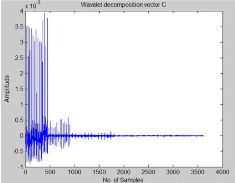
Figure 6 illustrates the decomposition coefficients in wavelet decomposition by “db3” wavelet family. The decomposition structure can be seen as decomposition tree. Figure 7 shows the tree decomposition of ECG signal. In this Figure 7 right side shows the decomposition structure at each node.

Figure 6. Decomposition at Multilevel (level=3 with “db3”).

Figure 7. Tree Decomposition (level=3 with “db3”).

Figure 8 describes approximation and detail coefficients of the signal after decomposition. Figure 9 describes the original and threshold signal which make a fixed percentage of coefficients equal to zero (global thersholding).

(10)

Figure 9. Original and Thresholding Signal with Global Thresholding.

The run-length encoding signal is shown in Figure 10. The encoding or compress signal is decoded as shown in Figure 11. Finally the decoded signal must be reconstructed to get the original signal.

Figure 10. Encoding Signal.

Figure 11. Decoding Signal.

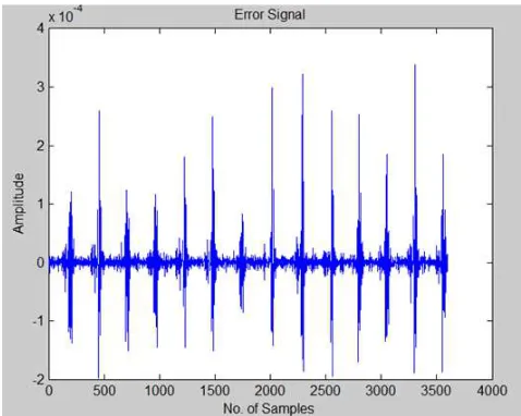
The reconstruction was almost lossless, and the only noticeable change in the reconstructed waveform was the elimination of noise in the ECG. Figure 12 shows the original and reconstructed waveforms of a ECG signal namely ‘Record 105’ from MIT-BIH database. Figure 13 illustrates the error signal between reconstructed and orignal ones of the ECG signal (Record 105) when the compression algorithm is adopted.

Figure 12. Original and Reconstructed Signal (Global Thresholding and “db3” Wavelet).

Figure 13. Error Signal (Global Thresholding and “db3” Wavelet).

(11)

Figure 14. Original and Thresholding Signal with Local Thresholding.

Figure 15. Original and Reconstructed Signal (Local Thresholding and “db3” Wavelet).

The compression technique with local thresholding method is also tested. The decomposition structure are the same as above section. The results of orginal signal 105 and thresholding signal by loacal thresholding method and “db3” are as shown in Figure 14. The original and reconstructed waveforms of a ECG signal is shown in Figure 15 and the error signal is in Figure 16.

Figure 16. Error Signal (Local Thresholding and “db3” Wavelet).

Figure 17. Original and Thresholding Signal (Record 205, Local Thresholding, “Haar” Wavelet).

Other ECG signals from MIT-BIH Database are tested with the wavelet family “Haar”, db4, db5 ect. The following Figureures show some of the results of various tests. Figure 17 shows original and thresholding signal (Record 205, local thresholding, “Haar” wavelet).

Figure 18. Original and Reconstructed Signal (Record 205, Local Thresholding, “Haar” Wavelet).

(12)

Figure 18 shows original and reconstructed signal (record 205, local thresholding, “Haar” wavelet). The error signal (record 205, local thresholding, “Haar” wavelet) is shown in Figure 19.

Figure 20. Original and Reconstructed Signal (Record 100, Global Thresholding, “db3” Wavelet).

Figure 20 shows original and reconstructed signal (record 100, global thresholding, “db3” wavelet).

The two thresholding methods were implemented on a MATLAB environment. The two methods were tested on the ECG data from the following MIT-BIH arrhythmia database files. Various criteria were used to evaluate the fidelity of reconstruction. Though Percent Root Difference (PRD) has been widely used in the literature as the principal error criterion, it highly underestimates the error in the presence of a d.c. shift, and averages out localized high errors in the QRS region. In this work, Signal to Noise Ratio (SNR) and Root Mean Square Error (RMSE) were used, in addition to PRD. These values are given along with the CR.

In order to make the results quantitatively comparable to the ECG compression methods, here, the most widely-used numerical indexes of PRD, compression ratio (CR) and signal to noise ratio (SNR) are adopted. The CR is used to measure the compression efficiency, which is defined by the ratio of the bits of the original data to those of the compressed data.

The Equations are used for evaluation of PRD and CR. Table 1 illustrated the performance of methodology for the ECG compression in form with the different wavelet transform and run-length encoding technique.

Table 1. Comparative Performance of the Two Thresholding Method for Different Wavelets.

ECG Signal

Wavelet Names

Local Thresholding Global Thresholding

CR PRD CR PRD

100

‘db3’ 7.6154 0.4151 2.2768 0.4130 ‘haar’ 10.7902 0.4275 5.2181 0.4224 ‘sym2’ 7.7374 0.4724 3.1414 0.4703 ‘coif1’ 7.7586 0.3976 2.9703 0.3951 ‘db10’ 7.4130 0.4499 2.9788 0.4480

ECG Signal

101

102

103

104

105

106

107

Table 2. Comparative Performance of the Two Thresholding Method for Different Wavelets.

CG Signal

108

‘haar’ 9.8287 0.1922 4.9581 0.1746 ‘sym2’ 7.5804 0.1314 2.8147 0.1154 ‘coif1’ 7.4972 0.1332 2.5070 0.1185 ‘db10’ 7.3524 0.1086 2.8002 0.0914

109

201

202

203

(13)

CG Signal

205

207

The criteria for testing the performance of the compression algorithms consist of three components: compression measure, reconstruction error and computational complexity. Fourteen record signals from MIT-BIH Database are tested with five mother wavelet names. Each signal is tested by two thresholding methods and five wavelets. Five wavelets (db3, db10, haar, sym2, coif1) are tested in this system. It can be seem that “haar” wavelet is the best compression ratio for both thresholding methods. Other four wavelets are different a little. The performance measurement comparisons are shown in the Table 1. Local thresholding method is applied in each decomposition level. Global thresholding method is applied the last level of decomposition. Therefore, local thresholding method is better than the global thresholding in every signal. Haar wavelet is the best compression ratio in all signals. The record signal name 205 gets the best compression ratio with local thresholding and “Haar” wavelet. In thresholding step, all coefficients less then “threshold vaule” are reduced to zero. The record signal 205 file is noisy signal. So, all noises are reduced to zero values by thresholding. The signal 100 does not contain noise. So the coefficient values that reduced to zero value by thresholding is a little. Therefore, the record signal 100 is the least compression ratio with global thresholding and “db3” wavelet.

10. Conclusion

In this research, a one-dimensional signal compression is described. The advantage of method is that the compression performance is higher with low signal quality degradation at the single level decomposition. Another advantage of the method is that all the information of signal is hidden because the signal is encoded. Therefore, this method is used at the transmission. It is securer because transmitted data are encoded with wavelet coefficients. Hence the method is applicable to the 1-D signal compression with more security. Results were obtained by running on different sets of data taken from MIT-BIH database. The results show that the proposed ECG data compression algorithm is capable of achieving good compression ratio values. The algorithm could compress all kinds of ECG data very efficiently, perhaps more efficiently than any previous ECG compression methods. The user can truncate the bit stream at any point and obtain the best quality of reconstruction for the truncated

file size. All compression solutions presented in this research adopt DWT as a reversible compression tool.

References

[1] Benzid R., Marir F., Boussaad A., Benyoucef M., and Arar D., Fixed percentage of wavelet coefficients to be zeroed for ECG compression, Electronics Letters, vol. 39, 830–831, 2003. [2] Chen, X., Wang W. and Wei. G, Impact of HTTP

Compression on the Web Response Time in Asymmetrical Wireless network, Proc. Of International Conference on Network Security, Wireless Communication and trusted Computing, Vol. 1, pp. 679-682, 2009.

[3] Liu, Z., Saifullah, Y., Greis M. and Sreemanthula, S., HTT Compression Techniques, IEEE conf. Proc. Of Wireless Communication and net working, Vol. 4, pp. 2495-2500, 2005. [4] A. G. Ramakrishna and S. Saha, ECG coding by

wavelet-based linear prediction, IEEE Trans. Biomed. Eng., Vol. 44, No. 12, pp. 1253–1261, 1997.

[5] Ajay Bharadwaj, Accurate ECG Signal Processing, Published in EE Times Design, February 2011. http://www.eetimes.com/design.

[6] S. M. Joseph., Spoken Digit Compression Using Wavelet Packet, IEEE Signal and Image Processing (ICSIP). pp. 255-259, Chennai, India, Dec. 15-17, 2010.

[7] Prof. Mohammed Abo-Zahhad, ECG Signal Compression Using Discrete Wavelet Transform, ISBN: 978-953-307-185-5, (2011).

[8] Storer, James A., Data Compression: Methods and Theory, Computer Science Press, Rockville, MD, 1988.

[9] Zou H. and Tewfik A. H., Parameterization of compactly supported orthonormal wavelets, IEEE Trans. on Signal Processing, vol. 41, no. 3, 1428-1431, March 1993.

[10] Zigel Y., Cohen A., and Katz A., The Weighted Diagnostic Distortion (WDD) Measure for ECG Signal Compression, IEEE Trans. Biomed. Eng., 47, 1422-1430, 2000.

[11] Abdelaziz Ouamri, ECG Compression method using Lorentzia function model, Science Direct, Digital Signal Processing 17, 8th August 2006.

[12] http://www.iki.fi/a1bert/.

[13] Anonyms, Data Compression, 21 October, (2012).

[14] http://en.wikibooks.org/wiki/DataCompression/Dictionarycom pression.

[15] Anonyms, Discrete Wavelet Transform, Sep 01, 2012. [16] http://www.thepolygoners.com/tutorials/dwavelet/DWTTut.ht

ml.

[17] Anubhuti Khare, Manish Saxena, Vijay B. Nerkar, “ECG Data Compression Using DWT”, Volume-1, Issue-1, October 2011.

(14)

[19] http://www.intechopen.com/books/discrete-wavelet- transforms-theory-and-applications/ecg-signal-compression-using-discrete-wavelet-transform.

[20] Pranob K Charles, Rajendra Prasad K, A Contemporary Approach for ECG Signal Compression using Wavelet Transforms”, Vol. 2, No. 1, March 2011.

[21] Ranjeet Kumar, Rajesh Gautam and Anil Kumar, HTTP Compression for 1-D signal based on Multiresolution Analysis and Run length Encoding, 2011 International Conference on Information and Electronics Engineering IPCSIT vol. 6, © IACSIT Press, Singapore. (2011).

[22] Vinod kumar Professor, Application of Wavelet Techniques in ECG Signal Processing: An Overview, ISSN: 0975-5462 Vol. 3 No. 10 October 2011. Mohammed Abo-Zahhad (2011). [23] Chun-Lin, Liu, A Tutorial of the Wavelet Transform, February

23, 2010.

[24] Abdelaziz Ouamri, Data Compression Techniques, Dec 2008. [25] Javaid R., Besar R., Abas F. S., Performance Evaluation of

Percent Root Mean Square Difference for ECG Signals Compression. Signal Processing, An International Journal (SPIJ), 1–9, April, 2008.

[26] A. Al-Shroud, M. Abo-Zahhad and S. M. Ahmed, A novel compression algorithm for electrocardiogram signals based on the linear prediction of the wavelet coefficients, Digital Signal Processing, Vol. 13, pp. 604–622, 2003.

[27] Ahmed S. M., Al-Shrouf A. and Abo-Zahhad M., ECG data compression optimal non-orthogonal wavelet transform, Med. Eng. Phys. 22, 39–46, 2000.

[28] Pasi Ojala Pasi 'Ojala, Compression Basics, 19.11.1997. [29] Jalaleddine SMS, Hutchens CG, Strattan RD, Coberly W A,