Phase Structure of Fluid Fluctuations with a Floating Elastic Ice Plate under Nonlinear Interaction of Progressive Surface Waves

Phase Structure of Fluid Fluctuations with a Floating Elastic Ice

Plate under Nonlinear Interaction of Progressive Surface Waves

A. E. Bukatov, A. A. Bukatov*

Marine Hydrophysical Institute, Russian Academy of Sciences, Sevastopol, Russian Federation *e-mail: [email protected]

Asymptotic expansions up to the third-order terms are constructed based on the multiple scales method for the fluid velocity potential of the finite-depth homogeneous fluid and elevation of the plate-fluid surface (ice-water surface). The obtained expansions constitute a foundation for analyzing dispersive properties of the fluctuations formed under interaction of progressive harmonics of the finite-amplitude surface waves. Changes of the fluctuation frequency taking place due to the contribution of the values of the first and second approximations conditioned by the taken into account non-linearity are considered. The effect of non-linearity of the ice plate vertical displacement acceleration on the amplitude, frequency and phase velocity of the wave disturbances is studied. It is shown that at the wave numbers exceeding the maximum resonance value, the oscillation frequency increases in case non-linearity of the plate vertical displacement acceleration is taken into account. It also grows with the plate thickness, and change of a sign (plus into minus) of the second interacting harmonic amplitude reduces the frequency value if the wave number is fixed. The phase velocity increase with allowance for the acceleration nonlinearity is more significant than without considering it. Under a negative amplitude of the second interacting harmonic, if the acceleration nonlinearity is taken into account, the phase velocity is less than when it is not.

Keywords: ice plate fluctuations, waves of finite amplitude, nonlinear interaction of waves, flexural deformation of plate, phase characteristics.

Acknowledgements. The present study is carried out within the framework of the State Order No. 0827-2018-0003.

For citation: Bukatov, A.E. and Bukatov, A.A., 2018. Phase Structure of Fluid Fluctuations with a Floating Elastic Ice Plate under Nonlinear Interaction of Progressive Surface Waves. Physical Oceanography, [e-journal] 25(1), pp. 3-17. doi:10.22449/1573-160X-2018-1-3-17

DOI: 10.22449/1573-160X-2018-1-3-17

© 2018, A. E. Bukatov, A. A. Bukatov

© Physical Oceanography

The fluctuations formed in the system of an ice plate – liquid under the interaction of harmonics of traveling periodic surface waves of finite amplitude are studied in the present paper.

1. Problem statement. Suppose a thin elastic plate of constant thickness h is floating on the surface of the homogeneous ideal incompressible fluid of constant depth H. In the horizontal directions, the plate and liquid are unlimited. Let us consider the nonlinear fluctuations of a plate in the interaction of the first and second harmonics of progressive waves of finite amplitude, assuming that the fluid movement is potential, and the plate fluctuations are uninterrupted. In dimensionless variables x=kx₁, z=kz₁, t= kgt₁, ζ=kζ∗, and ϕ=

(

k2 kg

)

ϕ∗, where k is the wave number; g is the gravity acceleration; t is the time; φ(x, z, t) is the fluid movement velocity potential; ζ(x, t) is the plate or the plate–fluid surface elevation, the problem involves the Laplace equation solution

ζ ,

,

0 −∞< <∞ − ≤ ≤

= ϕ +

ϕ_{xx zz} x H z (1.1)

for the velocity potential with boundary conditions on the plate–liquid surface (z = ζ)

p t x z k x k

D =

    

  

∂ ϕ ∂ −      

∂ ϕ ∂ ∂

∂ + ∂

∂ 2

4 4 4 1

2 1 κ

ζ _{, (1.2)}

    

  

     

∂ ϕ ∂ +      

∂ ϕ ∂ − ζ − ∂

ϕ ∂ =

2 2

2 1

z x

t p

and at the bottom (z = –H) of the basin

. 0

= ∂

ϕ ∂

z (1.3)

In the initial time (t = 0)

0 ζ ), (

ζ =

∂ ∂ =

t x

f . (1.4)

Here

ρ ρ κ ; ) ν 1 ( 12 ,

ρ

1 2

3

1 h

Eh D

g D

D =

− =

= ;

Е, h, ρ1 and ν are the normal elasticity module, thickness, density and Poisson's ratio of the plate; ρ is the fluid density. The velocity potential and deflection of the plate at z = ζ are bounded by the following kinematic condition

0

= ∂

ϕ ∂ + ∂

ϕ ∂ ∂

ζ ∂ − ∂

ζ ∂

z x x

t . (1.5) In the dynamic condition (1.2), the expression with the factor κ represents the inertia of the vertical displacements of the plate. The first term in the brackets of this expression characterizes the nonlinearity of the vertical acceleration of the plate.

2. Equations for nonlinear approximations. The problem solution (1.1)– (1.5) is obtained by the method of multiple scales [16]. Two new variables

t T t

T1=ε , 2 =ε2 are introduced. They are slowly varying in comparison with t = Т0, where ε is small but finite, and the validity of the expansions is assumed

), ε ( ζ ε εζ ζ ζ , ε , ε , εζ

ζ 3

3 2 2 1 0 0 0

0 ϕ= ϕ f = f = + + +O

= (2.1)

). ε ( ε

ε ),

ε ( ε

ε 3

3 2 2 1 0 3 3 2 2 1

0 =ϕ + ϕ + ϕ +O f = f + f + f +O

ϕ

Substituting φ from the expressions (2.1) into (1.1) and (1.3), within the accuracy up to the the third-order values, the following expression is obtained

2 2

2 2 3

3 2 2 1 3

3 2 2

1 ε ε 0, ε ε ε 0,

ε

z x z

z

z ∂

∂ + ∂

∂ = ∆ = ∂

ϕ ∂ + ∂

ϕ ∂ + ∂

ϕ ∂ = ϕ ∆ + ϕ ∆ + ϕ

∆ .

Below the dynamic (1.2), kinematic (1.5), and initial (1.4) conditions are considered. The surface velocity potential of a plate – liquid z=εζ0 is represented in the following form

... ) , 0 , ( ζ ε 2 1 ) , 0 , ( εζ ) , 0 , ( ) , εζ ,

( ₀ =ϕ + ₀ϕ + 2 2₀ϕ +

ϕ x t x t _z x t _zz x t . (2.2)

) , εζ , ( , ε , εζ

ζ= 0 f = f0 ϕ x 0 t and ϕz(x,εζ0,t) are substituted in the corresponding conditions (1.2) and (1.5), bearing in mind that, according to the complex function differentiation rule, the partial derivative with respect to time is defined by the following expression

2 2

1 0

ε ε

T T

T

t ∂

∂ + ∂

∂ + ∂

∂ = ∂

∂

,

taking into account the dependence of ζ0 on x and t in the expression (2.2). Then, collecting the coefficients at equal powers of ε and equating them to zero, the following equations are found

0 ,

, 0 2 2

2 2

≤ ≤ − ∞ < < ∞ − = ∂

ϕ ∂ + ∂

ϕ ∂

z H x

z x

n

n _{, (2.3)}

0 , *

0 0 2

4 4 4

1 _∂ +ζ = =

ϕ ∂ − ∂ ∂

ϕ ∂ κ − ∂

ζ ∂

z F T

T z k x k

D n n

n n

n _{, (2.4)}

0 , 0

= =

∂ ϕ ∂ + ∂

ζ ∂

z L z

T n

n

n _{, (2.5)}

H z z

n = =−

∂ ϕ ∂

,

0 , (2.6)

0 , ),

(

0

= =

∂ ζ ∂ =

ζ G t

T x

f n

n n

n (2.7)

for the determination of nonlinear approximations. Here

3 , 2 , 1 , 0

, 1 1

0 1 1 0

*_{= + = = = = =}

n G

L F F F F

kN z x z T T z T

F +κ

              ∂ ϕ ∂ +       ∂ ϕ ∂ − ∂ ϕ ∂ ∂ ζ ∂ + ∂ ϕ ∂ + ∂ ∂ ϕ ∂ ζ = 2 1 2 1 1 0 1 1 1 0 1 2 1 2 2 1 , , , 1 1 2 1 2 1 1 1 2 1 1 2 2 0 1 3 1 2 1 2 0 1 T z x x L z T z T z T N ∂ ζ ∂ − ∂ ϕ ∂ ζ − ∂ ϕ ∂ ∂ ζ ∂ = ∂ ∂ ϕ ∂ + ∂ ∂ ϕ ∂ ζ + ∂ ϕ ∂ ∂ ζ ∂ = 3 2 2 1 2 1 2 1 1 2 0 1 2 2 1 1

3 N kN

z z x x T T z T N

F + +κ

∂ ϕ ∂ ∂ ϕ ∂ − ∂ ϕ ∂ ∂ ϕ ∂ − ∂ ϕ ∂ + ∂ ϕ ∂ + ∂ ∂ ϕ ∂ ζ + ζ = , 2 0 1 3 1 1 0 1 2 1 2 1 1 2 0 2 2 1 1 2 1 2 1 z T z T z x x z z T z T N ∂ ∂ ϕ ∂ ζ +       ∂ ϕ ∂ − ∂ ζ ∂ ∂ ϕ ∂ + ∂ ϕ ∂ ∂ ∂ ϕ ∂ − ∂ ∂ ϕ ∂ + ∂ ∂ ϕ ∂ = ,       ∂ ϕ ∂ ∂ ζ ∂ − ∂ ζ ∂ + ∂ ζ ∂ ∂ ϕ ∂ + ∂ ϕ ∂ ∂ ζ ∂ = x x T T z z T

N 1 1

1 1 0 2 1 2 0 1 2 , , 2 1 5 2 1 2 1 1 0 2 2 1 2 2 0 1 3 2 3 0 1 4 2 1 4 1 3 N T z T T z z T z T N N + ∂ ∂ ϕ ∂ +       ∂ ζ ∂ + ∂ ζ ∂ ∂ ϕ ∂ + ∂ ∂ ϕ ∂ ζ + ∂ ∂ ϕ ∂ ζ + ζ = , , 1 2 2 2 2 2 0 1 5 1 2 1 3 3 1 3 0 1 2 0 2 3 4 T z z T N T z z T z T N ∂ ∂ ϕ ∂ + ∂ ϕ ∂ ∂ ζ ∂ = ∂ ∂ ϕ ∂ + ∂ ϕ ∂ ∂ ζ ∂ + ∂ ∂ ϕ ∂ = , 2 1 1 2 1 1 2 2 1 1 2 2 1 2 2 6 1 3       ∂ ζ ∂ ∂ ϕ ∂ + ∂ ζ ∂ − ∂ ζ ∂ − ∂ ϕ ∂ ∂ ζ ∂ + ∂ ϕ ∂ ∂ ζ ∂ + ∂ ϕ ∂ ζ − ζ = x z T T x x x x z N L , , 2

1 1 1

2 0 2 3 1 3 1 2 2 2 1 2 1 6 x z x k F z z x z x N ∂ ϕ ∂ ∂ ∂ ϕ ∂ κ − = ∂ ϕ ∂ ζ − ∂ ϕ ∂ − ∂ ∂ ϕ ∂ ∂ ζ ∂ = , 2 1 2 1 2 2 1 1 1 2 1 2 7 1 0 3               ∂ ϕ ∂ ∂ ζ ∂ + ∂ ∂ ϕ ∂ ∂ ϕ ∂ +       ∂ ϕ ∂ ∂ ζ ∂ + ∂ ϕ ∂ ∂ ∂ ϕ ∂ + ζ κ − = z x z x x z x x z x N k F . , , 1 2 2 1 3 1 1 2 2 1 3 1 2 1 2 7 T T G T G z x x z x N ∂ ζ ∂ − ∂ ζ ∂ − = ∂ ζ ∂ − = ∂ ∂ ϕ ∂ ∂ ϕ ∂ +       ∂ ∂ ϕ ∂ =

Note that F20_{and F3}0 _{terms appearing on the right-hand sides of the dynamic} conditions (2.4) for the second (n = 2) and third (n = 3) approximations are due to the nonlinearity of the vertical displacements of the plate.

3. Expressions for the plate deflection and the fluid movement velocity potential. The equations (2.3)–(2.7) are obtained for the general case of unsteady fluctuations of finite amplitude. Solution of these equations in the case of interaction of traveling periodic wave harmonics ζ11=cosθ andζ12=a1cos2θ,

) , ( _{1 2}

0 T T

T x+τ +β

=

θ is to be obtained. The first approximation (n = 1) of the surface elevation of the plate-liquid is defined in the form as

12 11 1=ζ +ζ

ζ , (3.1)

where a1 is the constant of the order of unity, and β = 0 under t = 0. Satisfying the condition at the bottom and taking into account the relationship of the wave characteristics through the boundary conditions (2.4), (2.5), the following can be written

(

)

(

)

  

 + _θ

+ θ +

τ =

ϕ sin2

2 sh 2 ch sin

sh ch

1 1

H H z a H

H z

, (3.2)

(

1 D1k4

)

(

1 kthH

)

1thH

2 _{= + +κ} −

τ .

Amplitude a1 and phase shift β (Т1, Т2) are determined from subsequent approximations.

Substituting ζ1 and φ1 in the right sides of the dynamic (2.4) and kinematic (2.5) equations for the second approximation and solving the problem (2.3)–(2.7) for n = 2, taking into account the requirement of absence of the first and second harmonics in the particular solution, ζ2 and φ2 are obtained. In turn, ζ1 and ϕ1 and

ζ2 and ϕ2 determine the right sides of the dynamic and kinematic conditions when n = 3. Eliminating the terms generating secularity from them, ζ3 and ϕ3 are obtained.

As a result, the basin surface elevation ζ and fluid movement velocity potential φ in dimensionless variables up to the third-order quantities are determined from following expressions

, cos cos

2 cos cos

6

5 3 3 3

1

4

3 3

2

∑

∑

∑

∑

=

= = =

θ ε

+ θ ε

+ θ ε

+ θ ε = ζ

n n

n j

j n n

n n

n

n a j

a

a (3.3)

(

+

)

θ+ ε

(

+

)

θ+

τ ε =

ϕ

∑

= 3

1

2ch2 sin2 sin

ch

sh _n n

n

H z b H

z H

(

z H

)

j b n

(

z H

)

n b t

j b

n n n

n n j

nj n

n

∑

∑

∑

∑

= =

= =

ε + θ +

ε + θ +

ε

+ 3

2 0 6

5 3 3 4

3 3

2

sin ch

sin

ch , (3.4)

, ,

, 2

2

1 ak

t

x+σ σ=τ+εσ +ε σ ε=

= θ

where а is the amplitude of the initial harmonic. Here

H a b

2 sh 1 12

τ

= ,

2 1

2 2 2

2

1 2 1

) 2 th 2 1 ( ) 4

2 cth 2 (

4 _

 

 

κ + µ + κ τ + τ

µ ±

=

H k k

H r

r

a , (3.5)

(

)

(

1

)

2

1 cth

2 5 3

cth 2 1 cth 2 th cth

2 _ τ +κ +µ

  

 

   

 

−    



 _{+ κ}

+

= H H H H k H k

r ,

   



 ₊

µ +    

 

   



 ₋

κ − +

τ

= H H k H H H H

r cth cth2

2 1 cth

2 5 2 cth cth

2 cth 2 1

1 2

) 2 th 2 1 )( 4 2 cth 2 ( 4 2 5 3 cth 2 1 cth 2 th cth 2 2 2 2 1 2 1 H k k H a k H H H H κ + µ + κ τ + τ             −       _{+ κ} + τµ = σ ,

(

H H

)

a

l 2cth2 cth

2 3

1

3 =− τ + , l 4a cth2H 2 1

4=− ,

            ₋ κ + − τ

=a H H k H H

l cth 2 1 2 cth 5 cth 2 cth 2 11 2 1 7 ,

(

H k H

)

a

l₈ = ₁2τ2 5−cth22 +4κ cth2 ,

) 3 cth 3 9 ( 3 sh 3 3 2 2 3 7 3 3 23 H k H l l b τ − τ κ − µ τ + µ = , ) 4 cth 4 16 ( 4 sh 3 4 2 2 4 8 4 4 24 H k H l l b τ − τ κ − µ τ + µ = ,

(

)

(

l b H k H

)

a₂₃ =µ−₃1 ₇+3τ ₂₃ ch3 −κ 3sh3 ,

(

)

(

l b H k H

)

a 8 4 24 ch4 4sh4

1 4

24 =µ + τ −κ

− , 1 23 24 24 2 1

3 cth 3

2 3 4 ch 6 8 3 8 5 σ + τ − − τ − τ −

= a b H a H a

j , 1 24 23 23 1

4 6 ch3 2 cth 4

2

9 _{τ− − τ + σ}

−

= a b H a H a

j ,       _{− τ} − τ − − τ −

= a b H a H a b H a H

j ch3 cth2

2 3 5 cth 2 5 4 ch 10 8 69 23 23 1 24 24 2 1 5 ,

(

b H a H

)

a a

j 5 6 1 2 24ch4 24 cth2

3 1

6=− τ− − τ ,

(

)

(

)

(

)

(

(

, 3 sh 9 cth 2 1 cth 2 3 8 1 2 cth cth 2 7 2 cth 2 8 21 cth 2 1 2 2cth 3 cth 4 4 cth 11 4 sh 2 3 ch 3 3 2 cth 7 23 1 cth 4 1 2 1 cth 4 th 2 4 ch 2 2 9 1 23 2 24 2 2 1 2 1 1 24 1 23 24 2 1 2 1 2 24 1 1 3    σ +    −    − − −       _{− −} τ +       ₊ + + σ + − τ κ + σ +    −    _{− +} τ +       _{σ + −} τ = H b H H a H H H a H H a H H H b k H b a H a a H H H H b a m

(

)

(

)

, 4 sh 16 cth 2 cth 4 3 cth 2 cth 4 4 37 2 cth 8 cth 3 3 cth 11 3 sh 2 3 4 ch 4 cth 4 1 2 cth 2 cth 3 th 5 3 ch 2 3 4 1 24 23 2 1 2 1 2 1 23 1 24 23 1 1 2 23 2 1 1 4    σ +       +       _{− −} τ + +          _{− + σ} τ κ + σ + +       _{− +} τ +       _{σ + −} τ = H b H a H H H a H a H H H b k H b a H a H a H H H b a m

(

)

(

)

(

, cth 2 5 2 cth 10 cth 2 cth 2 11 2 cth 6 8 3 2 cth 3 3 cth 2 11 3 sh 3 cth 4 4 cth 19 4 sh 2 2 5 5 cth 8 7 2 cth 2 7 2 cth 3 th 2 7 3 ch 3 cth 4 th 6 4 ch 2 24 1 23 2 1 2 1 23 24 24 1 23 2 1 2 1 2 1 23 24 5       + +    ₊       _{− −} τ +          ₋ +   _{τ − +} κ +       _{− + +} τ + +             ₋ + − τ = H a H a a H H H a H H H a b H H H b k a a a H a H a H H H a b H H H b m

(

)

(

)

(

)

(

(

)

)

(

4 sh4 5cth4 2cth2 6 cth2 1 4cth 2

)

,

2 6 2 cth 2 cth 4 th 4 4 ch 4 2 2 1 24 2 24 1 24 2 1 1 2 1 24 6 H a H a H H H b ka a H a a H H H a b m + − τ + − τ κ + + + τ + − τ = , 4 39 2 cth cth 2 cth 8 8 3 cth 2 1 cth2 2 cth 2 1 2 cth 2 2 cth 3 3 cth 2 1 3 sh 3 2 5 cth 4 1 2 cth 9 2 cth 3 th 2 1 3 ch 3 2 1 2 cth 4 15 8 3 3 ch 2 3 2 2 1 2 2 1 23 3 1 1 23 1 2 2 1 23 1 2 1 3 23 1 1 2 1 23 2 1 1 23 1 1                _{+ +} + + τ + τ +    +       σ + σ −       ₊ τ κ + +             − + + τ +          ₊ +   _{− σ +} τ +             _{− +} τ − µ = H H H a H H a a H H H H H b a k a H a a H a H H H b a H a a a H a b q

(

)

(

)

(

)

(

)

(

)

(

)

(

)

(

)

(

)

(

)

cth ,

6 ... 3 , ) cth ( sh , 2 4 1 2 2 2 3 2 1 2 1 1 2 = τ − κ τ − µ τ + µ =       µ + µ = σ n nH n k n nH n nm j b a q q n n n n n ,

(

)

(

3 ch 3 sh

)

1, 3...6

3 = τ + κ + µ =

− n m nH k nH b n

an n n n ,

4 1 4 1 n Dk

n = +

µ , n = 1...6,

(

) (

)

_            ₊ κ + + + + τ

= a H H k H a H

b cth 4 cth2

2 1 cth 1 4 1 2 cth

1 12

2 2 2 1 2 20 ,             _{+ −} κ + + τ

=a H H k H H H

b30 1 2 cth2

4 1 cth 2 cth 2 4 9 cth 2 1 2 cth 2 .

Wherein b22=b32=a2 =a3 =l1=l2=l5 =l6= j1= j2=m1=m2 =0.

Formulas (3.3) – (3.4) for ζ and φ determine the wave disturbance being formed, and in case the nonlinearity of the vertical displacement acceleration of ice in the dynamic condition (2.4) is not taken into account. However, in this case it should be taken into account that

      ₊ µ +             ₊ κ − + τ

= H H k H H H H

r cth cth2

2 1 cth 2 1 2 cth 2 cth 2 cth 2 1 1 2 2 ,             ₋ κ + − τ

=a H H k H H

l cth 2 3 2 cth 6 cth 2 cth 2 11 2 1 7 ,

(

)

)

)

, 3 sh 9 4 ch 24 cth 4 1 4 15 2 3 2 cth 2 cth 2 1 3 3 ch 3 3 cth 4 1 cth 4 23 2 cth 7 2 1 2 9 cth 4 th 2 4 ch 2 1 23 24 24 2 1 1 1 1 23 24 2 1 2 1 1 24 3 H b H b H a a H H a k H b a H H H a a H H H b m σ + + +          _{+ −} τ +       ₊ σ τ κ + σ + −    _{+ −}       ₋ τ +       _{− + σ} τ =

(

)

(

)

(

)

(

)

, 4 sh 16 cth 2 5 2 cth 4 3 ch 9 2 4 ch 4 cth 4 1 2 cth 2 4 cth 5th3 3 ch 2 3 1 24 23 1 1 2 1 23 1 24 23 1 2 2 1 1 23 4 H b H a a H a H b k H b a H H a a H H H b m σ + + + τ + σ + τ κ + σ + +       +       ₋ τ +       _{− + σ} τ =

(

)

, cth 2 1 2 cth 2 8 17 3 ch 2 9 4 ch 8 5 2 1 5 cth 4 1 2 cth 2 7 2 cth 3 th 2 7 3 ch 3 cth 4 th 6 4 ch 2 24 1 23 2 1 1 23 24 24 1 23 2 1 2 1 23 24 5          _{+ +} τ +    _{+ +} τ κ +             ₊ +       ₋ τ + +             ₋ + − τ = H a H a a a H a b H b k a a a H H a H H H a b H H H b m

(

)

(

)

(

)

(

48 ch4 6 12 cth2

)

,

6 2 cth 2 cth 4 th 4 4 ch 4 24 2 1 24 1 24 2 1 1 2 1 24 6 H a a H b ka a H a a H H H a b m + τ + τ κ + + + τ + − τ =

)

, 8 1 2 cth 2 4 1 cth 2 1 2 cth 2 3 ch 2 9 2 cth 9 2 5 cth 4 1 2 1 2 cth 3 th 2 1 3 ch 3 3 ch 2 3 2 cth 4 15 8 3 1 23 2 1 1 23 1 2 23 1 2 1 2 1 3 1 23 2 1 23 23 1 1 1 1             _{− +} τ +             ₋ σ + τ κ − −       + +       − τ +    σ − +       ₊ τ +             _{τ+ τ +} − τ − µ = H a a a H H H b a k a a H a a H H H H b a H b H a a a q

(

)

(

)

(

)

(

(

)

(

)

)

(

(

)

(

2 4 1 cth2 cth

))

,

cth 4 ch 16 3 ch 9 2 2 cth 4 cth 3 2 cth 5 2 2 cth 3 th 3 ch 3 4 ch 2 cth 8 2 cth 2 cth 4 ch 4 3 3 ch 3 23 24 1 3 1 1 24 1 23 2 23 24 1 1 2 1 3 1 23 1 24 2 1 24 23 1 24 3 1 23 2 2 H a H a a a H H b a H b k a H a a H H a a H H H b H H a b H a a H a H a b a H b q − − + τ + + σ + + τ κ − + − + + + τ + σ − − − τ + + τ + τ + + τ − µ = . cth 2 1 2 cth 2 2 1 30       ₊ τ

=a H H

b

In dimension variables (ζ*, φ*_, х

1, z1, t1, a) the following is obtained

(

)

(

)

, 6 cos 5 cos 4 cos 3 cos 2 cos cos 36 2 2 35 2 3 34 2 3 24 2 33 2 3 23 2 1 θ + θ + + θ + + θ + + θ + θ = ζ a k a a k a a k a ka a a k a ka a aa a (3.6)

(

)

(

)

(

(

)

(

)

)

(

(

)

(

)

(

)

sin5 ch6

(

)

)

,

5 ch 4 sin 4 ch 3 sin 3 ch 4 sin 4 ch 3 ch 2 sin 2 ch sin ch sh 30 36 35 34 33 3 20 24 23 2 12 2 1 t b H z b H z b H z b H z b kg k a t b H z b H z b kg a H z b H z H k g a + + + θ + + + θ + + θ + + + θ + + + + +       τ _{+ θ+ + θ}       = ϕ

(

ak a k

)

t

kg

kx 2

2 2

1+ σ

σ + τ + = θ .

Here and below, the index 1 for Latin symbols x, z, t and the asterisk sign for Greek ζи ϕ are omitted.

4. Analysis of the results. The obtained solution (3.6) is valid outward small neighborhoods of the resonance values of the wave number k, which are positive real roots k = k1, k = k2, k = k3, k = k4 of the equations

6 ... 3 , 0 cth 2 2

2_{τ κ − τ = =}

−

µn n k n nH n (4.1)

respectively. Wherein k1 > k2 > k3 > k4. Note that one of these resonance values k = = k1, obtained from the equation (4.1) when n = 3, coincides with the smaller of the two resonance values obtained in the case when the first approximation ζ1 is given in the form ζ1 = ζ11 [14].

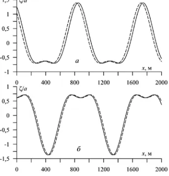
Fig. 1 and 2 show the ice-water surface elevation profiles (ice plate bending) along the direction of the wave propagation (negative direction of the x-axis) for E = 3·103 N/m2 _{and the values h = 1 m,} Н _{= 100 m when t = 17 min, k = 0.21 m}-1_, ε ₌ аk _{= 0.21} (Fig. 1) and t = 10 h, k = 7⋅10-3 _m-1_, ε_{= 1.4}⋅₁₀-2 _{(Fig. 2). The profiles} ζ₍х_{) in Fig. 1, a} and 2, a correspond to a positive value of the amplitude of the second interacting harmonic (а1> 0); in Fig. 1, b and 2b – to the negative one (а1< 0). Dashed lines are the profiles obtained taking into account the nonlinearity of the vertical displacement acceleration of the ice plate (F20≠ _{0, F3}0≠ _{0), and solid ones – without taking into} account (F20 _{= 0, F3}0 _{= 0).}

Fig. 1. The wave profiles of the flexural deformation of the ice plate with the amplitude of the initial harmonic a = 1 m and wave number k = 0.21 m-1_{, in case a}

1> 0 (а) and a1< 0 (b)

Fig. 2. The wave profiles of the flexural deformation of the ice plate with the amplitude of the initial harmonic а = 2 m and wave number 7⋅10-3 _m-1_{, in case a}

1> 0 (а) and a1< 0 (b)

From the analysis of ζ(х) graphs, it follows that under the interaction of wave harmonics, the nonlinearity of vertical displacement acceleration of the ice plate during its flexural deformation hastens the wave profile displacement in the negative direction of the x axis (the direction of wave motion) and slightly changes the amplitude of the flexural wave, depending on the wave number and the characteristics of the plate. When а1 > 0 the maximum displacements of the basin surface are reached at the tops of the wave elevations, and the minimum ones – in the soles of the troughs. Variation of the sign of the amplitude а1 of the second interacting harmonic causes a substantial deformation of the flexural profile. In the case of а1< 0, the maximum profile displacements appear in the form of troughs. In this case, taking into account the nonlinearity of vertical displacement acceleration of the plate during the flexion causes the slowing down of the wave propagation velocity. As the wavelength of the fundamental harmonic increases, the contribution of the higher harmonics in the troughs and elevations on the profiles of ζ(х) becomes more notable, and with its decrease – the wave profile approaches the harmonic form.

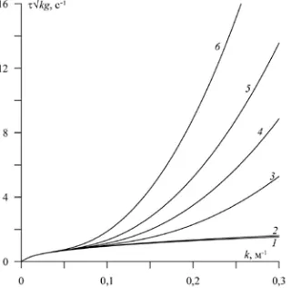
Distribution of the fluctuation frequency in the linear case and due to the frequency displacement nonlinearity in the approximation of the order of smallness of ε and in the approximation of order ε2 _{is shown in Fig. 3, 4 and 5, respectively,}

when H = 100 m. In Fig. 3 the curves 1, 3 and 4 are obtained when h = 0.5 m, and the curves 2, 5 and 6 – when h = 1 m. The lines 3, 5 correspond to the modulus of elasticity E = 109 _N/m2_{, and the lines 4, 6 – to the value E = 3}⋅₁₀9 _N/m2_{. Curves 1,} 2 correspond to the case of an absolutely flexible plate (E = 0) simulating broken ice. The graphs above show an increase in the linear component of the fluctuation frequency with increasing of the ice thickness and its modulus of elasticity, which agrees with [9, 17]. The shorter the wavelength (larger value of the wave number), the more pronounced the influence of h and E is. In the long wavelength range, it is practically absent.

Fig. 3. Distribution of the fluctuation frequency with respect to the wave number in the linear case with an ice thickness 0.5 m (the curves 1, 3, 4) and 1 m (the curves 2, 5, 6) in the case of the elastic modulus E = 109 _N/m2 _{(the curves 3, 5),}

E = 3⋅109 _N/m2 _{(the curves 4, 6), E = 0 (the}

curves 1, 2)

Fig. 4. Distribution of the vibration frequency component due to the nonlinearity in the first approximation, without taking into account the factor ε = ak in case a1> 0 when h = 0,5 m (the

curves 1, 2) and h = 1 m (the curves 3, 4), if E = = 109 _N/m2 _{(the curves 1, 3) and E = 3}⋅₁₀9 _N/m2

(the curves 2, 4)

Distribution of the nonlinearity dependent component of the fluctuation frequency with respect to the wave number in the approximation of order ε, without taking into account the factor ε = ak, is shown in Fig. 4 for а1 > 0, where the curves 1, 2 correspond to h = 0.5 m, and the curves 3, 4 – to the value h = 1 m. Curves 1, 3 were obtained when E = 109 _N/m2_{, and curves 2, 4 – when E =} = 3⋅109 _N/m2_{. The dashed lines are constructed when the nonlinearity of vertical} displacement acceleration of the plate is taken into account, and the solid lines – when it is not. From the figure, it can be seen that the acceleration nonlinearity effect (F20≠ _{0, F3}0≠ _{0) is manifested in an increase in the frequency displacement} component in the approximation of order ε. Moreover, the contribution of accounting for the acceleration nonlinearity increases with increasing the wave number (wavelength decrease). In case when а1 < 0, the given component value is preserved, but the sign changes to the opposite one. It can be seen from the expression σ1, where а1 is present in the denominator. Consequently, a change of а1 sign leads to a change in σ1 sign.

Dispersion curves connecting the displacement component of the second-order frequency with the wave number are shown within the accuracy of a factor of ε2 ₌ = a2_k2 _{in Fig. 5 for fixed} ε _{in the case a1}> _{0. At that, in Fig. 5, a they are given for} the wave number values from the range k <k4, and in Fig. 5, b – for k from the range k>k1. All the indications in Fig. 5 are the same as in Fig. 4. Behavior of the graphs indicates that in the range k <k4 there is a wave number value, passing through which the sign of the component of the order ε2 _{changes from plus to minus.}

In the range k>k1 this component is negative under the considered values of k. Taking into account the nonlinearity of vertical displacement acceleration of the plate reduces the component modulus value under a fixed value of k. The plate elasticity increase leads to an increase in the absolute value of the displacement frequency. A similar effect is observed with increasing thickness of the ice plate. The distribution character of the second-order displacement frequency with respect to the wave number under a fixed ε for a1< 0 is qualitatively the same as under a1> 0 (Fig. 5).

Fig. 6. Distribution of the fluctuations frequency formed in the case of nonlinear interaction of wave harmonics, by wavenumber when a1> 0 (the lines

1, 3) and a1< 0 (the lines 2, 4), in case h = 1 m (the

lines и 1, 2) and h = 0,5 m (the lines 3, 4)

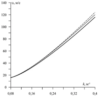
Fig. 7. The influence of taking into account the nonlinearity of vertical displacement acceleration of the plate on the phase velocity of the generated flexural-gravitational wave

Distribution of the fluctuations frequency

(

(

2

)

)

2 2

1+ σ

σ + τ =

σ kg ak a k

formed in the nonlinear interaction of wave harmonics is shown in Fig. 6. Here, the lines 1, 3 are given for a1 > 0, and the lines 2, 4 – for a1 < 0. The lines 1, 2 correspond to a plate thickness of 1 m and the lines 3, 4 – to the thickness of 0.5 m. The dashed curves show distribution frequency of the fluctuations with allowance for the nonlinearity of vertical displacement acceleration of the plate during its flexural deformation, and the solid ones without taking it into account. As expected, taking into consideration the acceleration nonlinearity leads to the fluctuation frequency increase. σ also grows with increasing of the elastic plate thickness. The change in the sign of the amplitude a1 from plus to minus decreases the fluctuation frequency value under a fixed wave number.

Influence of the consideration of the nonlinearity of vertical displacement acceleration of the plate during its flexion to the phase velocity of the formed finite amplitude flexural-gravitational wave is demonstrated by the graphs υ(k) shown in Fig. 7 for k > k1. They are obtained when a1 > 0, H = 100 m, h = 1 m, E = = 3⋅109 _N/m2_{, both taking into account (dashed line) and without taking into} account (thin solid line) the vertical acceleration nonlinearity. A thick solid line represents the phase velocity in the linear approximation. Analysis of the results of numerical calculations in the range of considered wave numbers shows that taking into account nonlinearity causes an increase in the displacement velocity of the flexural wave. At the same time, the increase in velocity with allowance for the nonlinearity of vertical displacements is greater than without taking it into account. Note that the value of the phase velocity increases with increasing of plate thickness or modulus of elasticity [9, 17].

If a1< 0, values of υ(k) if the acceleration nonlinearity is taken into account are less than without taking it into account. In this case, υ(k), both with and without allowance for acceleration nonlinearity, assumes smaller values than in the linear approximation.

In the range of wave numbers k < k4 (long waves), the influence of plate characteristics on the distribution of υ over k is not practically manifested [9, 17]. The dependences of υ υ(k) with and without allowance for the terms F20 _{and F3}0 _in the expression (2.4) coincide between each other both for a1> 0 and a1< 0. In the case a1> 0, the graph of υ(k) passes above the corresponding approximation, and in the case of a1 < 0 it is lower, although insignificantly.

displacements acceleration of the plate is manifested in the increase of this frequency displacement component.

Taking into account the nonlinearity of vertical displacement acceleration of the plate reduces the value of the modulus of the second-order smallness displacement component. Increase of the plate elasticity (or thickness) leads to an increase in the absolute value of this component.

Fluctuation frequency, taking into account the displacement components nonlinearity under the wave numbers larger than the maximum critical value, increases with allowance for the nonlinearity in the vertical displacement acceleration of the plate. The frequency also grows with the plate thickness increase. The second harmonic amplitude sign change from plus to minus decreases the frequency value under a fixed wave number. In this range of the wave numbers, the nonlinearity causes an increase in the velocity of flexural wave displacement under a positive second harmonic amplitude. The growth of velocity with allowance for the nonlinearity of vertical displacement acceleration is greater than without taking it into account. If the second harmonic amplitude is negative, and the acceleration nonlinearity is taken into account, the phase velocity is less than without it is not.

In the long-wave range under the wave numbers less than the minimum critical value, the influence of plate characteristics on the phase velocity distribution by the wave number is not practically manifested. The phase velocity distributions along the wavelength with and without allowance for the acceleration nonlinearity coincide with each other both for positive and for negative values of the second harmonic amplitude. Moreover, for a positive value of the amplitude, the phase velocity is greater, and for a negative value, it is less than in the linear approximation.

REFERENCES

1. Heysin, D.E., 1962. Nestatsionarnaya Zadacha o Kolebaniyakh Beskonechnoy Plastinki, Plavayushchey na Poverkhnosti Ideal'noy Zhidkosti [Non-Stationary Problem of Infinite Plate Fluctuations Floating on the Ideal Fluid Surface]. Izvestiya AN SSSR, OTN. Mekhanika i Mashinostroyenie, (1), pp.163-167 (in Russian).

2. Tkachenko, V.A. and Yakovlev, V.V., 1984. Neustanovivshiesya Izgibno-Gravitatsionnye Volny v Sisteme Zhidkost'-Plastinka [Unsteady Flexural Gravitational Waves in the Liquid-Plate System]. Prikladnaya Mekhanika, 20(3), pp. 70-75 (in Russian).

3. Squire, V.A., 1984. A Theoretical, Laboratory and Field Study of Ice-Coupled Waves. J. Geophys. Res., [e-journal] 89(C5), pp. 8069-8079. doi:10.1029/JC089iC05p08069

4. Schulkes, R.M.S.M. and Sneyd, A.D., 1988. Time-Dependent Response of Floating Ice to a Steadily Moving Load. J. Fluid Mech., [e-journal] (186), pp. 25-46. doi:10.1017/S0022112088000023

5. Duffy, D.G., 1991. The Response of Floating Ice to a Moving, Vibrating Load. Cold Reg. Sci. Technol., [e-journal] 20, (1), pp. 51-64. doi:10.1016/0165-232X(91)90056-M

6. Squire, V.A., Hosking, R.J., Kerr, A.D. and Langhorne, P. J., 1996. Moving Loads on Ice Plates. In: SMIA. Dordrecht: Kluwer Academic Publishers. Vol. 45, 236 p. doi:10.1007/978-94-009-1649-4

7. Pogorelova, A.V. and Kozin, V.M., 2010. Flexural-Gravity Waves due to Unsteady Motion of Point Source under a Floating Plate in Fluid of Finite Depth. J. Hydrodynam., 22(5), Suppl. 1, pp. 71-76. doi:10.1016/S1001-6058(09)60172-4

8. Sturova, I.V., 2007. Vliyanie Ledyanogo Pokrova na Kolebaniya Zhidkosti v Zamknutom Basseyne [Ice Cover Effect on Fluid Fluctuations in the Closed Basin]. Izvestiya. Atmospheric and Oceanic Physics, 43(1), pp. 128-135 (in Russian).

9. Bukatov, A.E. and Cherkesov, L.V., 1970. Transient Vibrations of an Elastic Plate Floating on a Liquid Surface. Soviet Applied Mechanics, 6(8), pp. 878-883. doi:10.1007/BF00889434 10. Bukatov, A.E. and Bukatov, A.A., 1999. Propagation of Surface Waves of Finite Amplitude

in a Basin with Floating Broken Ice. Int. J. Offshore Polar, 9(3), pp. 161-166.

11. Gol'dshteyn, R.V. and Marchenko, A.V., 1989. O Dlinnykh Volnakh v Sisteme Ledyanoy Pokrov – Zhidkost' pri Nalichii Ledovogo Szhatiya. Elektrofizicheskie i Fiziko-Mekhani-cheskie Svoystva L'da [Long Waves in the System Ice Cover – Liquid with Ice Compression. Electrophysical and Physico-Mechanical Properties of Ice]. Leningrad: Gidrometeoizdat, pp. 188-205 (in Russian).

12. Gladun, O.M. and Fedosenko, V.S., 1989. Nelineynye Ustanovivshiesya Kolebaniya Uprugoy Plastiny, Plavayushchey na Poverkhnosti Zhidkosti Konechnoy Glubiny [Nonlinear Steady Fluctuations of the Elastic Plate Floating on the Surface of the Liquid of the Ultimate Depth]. Izvestiya AN SSSR. Mekhanika Zhidkosti i Gaza, (3), pp. 146-154 (in Russian).

13. Il'ichev, A.T., 2015. Soliton-Like Structures on a Water-Ice Interface Uspekhi. Russian Mathematical Surveys, 70(6), pp. 1051-1103. doi:10.1070/RM2015v070n06ABEH004974 14. Bukatov, A.E. and Bukatov, A.A., 2009. Finite-Amplitude Waves in a Homogeneous Fluid

with a Floating Elastic Plate. J. Appl. Mech. Tech. Phy., [e-journal] 50(5), pp. 785-791. doi: 10.1007/s10808-009-0107-x

15. Bukatov, A.E. and Bukatov, A.A., 2003. Interaction of Surface Waves in a Basin with Floating Broken Ice. Physical Oceanography, [e-journal] 13(6), pp. 313-332. doi:10.1023/B:POCE.0000013230.35798.a4

16. Nayfe, A.Kh., 1976. Metody Vozmushcheniy [Methods of Perturbations]. Moscow: Mir, 455 p. (in Russian).

17. Heysin, D.E., 1967. Dinamika Ledyanogo Pokrova [Ice Cover Dynamics]. Leningrad: Gidrometeoizdat, 215 p. (in Russian).

About the authors:

Aleksei E. Bukatov, Head of Oceanography Department, FSBSI MHI (Sevastopol, Russia), Dr.Sci. (Phys.-Math.), Professor, ORCID ID: 0000-0001-8666-7938.

Anton A. Bukatov, Senior Researcher, Department of Marine Information Systems and Technologies, FSBSI MHI (Sevastopol, Russia), Ph.D. (Phys.-Math.), ORCID ID: 0000-0002-1165-8428, [email protected].

Contribution of the co-authors:

Aleksei E. Bukatov – scientific guidance, formulated and statement of the problem,

analysis and revision of the text.

Anton A. Bukatov – statement of the problem, derivation of an analytical solution,

analysis, reviewing the literature.