COMPARISON OF THE EQUATIONS OF STATE FROM JOULE-THOMSON
COEFFICIENT
G. A. Parsafar
1*, E. Noparast and E. Keshavarzi
1
Department of Chemistry, Isfahan University of Technology, Isfahan, Islamic Republic of Iran
Abstract
In the present work, we have examined the ability of some different equations
of state in predicting the Joule-Thomson coefficient,
μ
J-T, of different fluids. For
dense fluids, for which density is greater than the Boyle density,
ρ
B, two
appropriate equations of state, namely the linear isotherm regularity, LIR, and the
dense system equation of state, DSEOS, have been examined. The results show
that the DSEOS is in better agreement with the experimental data than the LIR.
However, only at very high pressures the LIR gives a better result. For low
densities, densities lower than the Boyle density, twelve equations of state namely
the van der Waals, Dieterici, Bertholet, Deiters, Virial, Adachi-Lu-Sugie,
Kubic-Marthin, Yu-Lu, Twu-Coon-Cunningham, Song-Mason, Ihm-Song-Mason, and
the extended linear isotherm regularity, ELIR, have been examined. The results
show that the Virial, Song-Mason, Ihm-Song-Mason and ELIR are in a better
agreement than the others. Finally we have recommended an appropriate equation
of state (ELIR) from which the Joule-Thomson coefficient can be calculated. In
this way we found that two harmless refrigerants, R-152a and R-32, have the
largest value of
μ
B
J-T
, which is in accordance with the experimental observations.
*E-mail: [email protected]
Introduction
The Joule-Thomson expansion is widely used for liquefaction and refrigeration of gases. The determination of the expansion condition is very important in the design of low temperature separation liquefaction plants and in the transport of natural gas processes. The expansion condition indicates whether the system is undergoing a heating or cooling process. It is also important to obtain μJ-T by using a theoretical
Keywords: Equation of state; Joule-Thomson coefficient; Refrigerants
In the present work, we evaluated different equations of state of predicting the Joule-Thomson coefficient. Owing to the fact that the Joule-Thomson coefficient is very sensitive to small deviations in temperature and pressure, it is a severe test [4] for the accuracy of the equation of state. There is no accurate equation of state, EOS, valid over an entire range of temperature and pressure. Here, the calculation of Joule-Thomson coefficient is divided into two different density ranges, densities greater than and those lower than the Boyle density. Appropriate equations of state for each range have been examined and compared. Finally, we have used more suitable equations of state to predict μJ-T for some refrigerants and from such a prediction we have proposed appropriate refrigerants which have a large value of μJ-T and a minimal amount of environmental damage.
Appropriate Equations of State for Dense Systems
The Joule-Thomson coefficient in terms of thermodynamic variables is,
⎥ ⎥ ⎥ ⎥ ⎦ ⎤ ⎢ ⎢ ⎢ ⎢ ⎣ ⎡ − ⎟ ⎠ ⎞ ⎜ ⎝ ⎛ ∂ ∂ ⎟ ⎠ ⎞ ⎜ ⎝ ⎛ ∂ ∂ − = − v v P T P T c T v p T J 1
μ (1)
where, p, v, T, and cp are pressure, molar volume, absolute temperature and specific heat capacity at constant pressure, respectively. The method of calculation is as follows:
Using a given equation of state, the expression for
v T P ⎟ ⎠ ⎞ ⎜ ⎝ ⎛ ∂
∂ and
T v P ⎟ ⎠ ⎞ ⎜ ⎝ ⎛ ∂
∂ can be obtained and substituted in
Equation 1, along with the experimental value of cp. For densities greater than the Boyle density we have used the LIR and DSEOS equations of state, because of their simplicity and knowledge of mathematical expressions for the temperature dependencies of their parameters [5,6]. According to the LIR, (Z-1)v2 is linear
versus ρ2 for each isotherm [5] as,
(Z−1)v2 =A+Bρ2 (2)
where Z=P/ρ RT is the compressibility factor, ρ =1/v is
the molar density, A and B are temperature dependent
parameters as, RT B B RT A A
A= 2 − 1/ , = 1/ (3)
and A1 and B
⎥ ⎦ ⎤ ⎢ ⎣ ⎡ + − + − − = − 4 1 1 2 2 2 1 2 1 5 ) ( 3 ) 5 2 3 ( 1 ρ ρ ρ ρ μ B A RT A RT B RT A A cp T
J (4)
The other suitable EOS for such a density range is the DSEOS. It predicts that ρv2 is quadratic versus ρ for
each isotherm as [6],
2 2 1 0
2 ρ ρ
ρv =A +A +A (5)
where A0, A1, and A2 are temperature dependent
parameters defined as,
2 , 1 , 0 ln )
(T =a +bT+cT2−dT T i=
Ai i i i i (6)
The values of constants ai, bi, ci, and di may be obtained from a least square fit of the experimental
ρ-v-T data in Equation 5, then the results obtained for
Ais may be fitted into Equation 6. This EOS is valid for densities greater than the Boyle density and dose not have any temperature limitation [6]. According to the DSEOS, μJ-T is given as,
⎥ ⎦ ⎤ ⎢ ⎣ ⎡ + + + + − ′ + ′ + ′ × − ) 4 3 2 ( 4 3 2 ( ) ( 1 3 2 2 1 0 2 2 1 0 2 2 1 0 ρ ρ ρ ρ ρ ρ ρ μ A A A A A A A A A T cp T J (7) where dT dA A i
i′= .
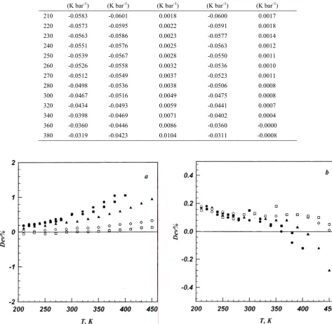
These two equations of state (LIR and DSEOS) are compared with the experimental data through their ability for predicting μJ-T. Because the experimental values of μJ-T are not reported for such a density range, we have used Goodwin’s μJ-T reported data for toluene which is calculated by an accurate EOS [8]. The values of μJ-T for toluene at 1.01325, 70, 250, 700, and 1000 bar are calculated. The results for 1.01325 bar are given in Table 1 and for other isobars are summarized in Figure 1 in which percent deviation is plotted versus temperature for LIR, Figure 1a and DSEOS Figure 1b. The agreement between the DSEOS and Goodwin’s reported values is quite well. We may conclude that the DSEOS can predict μJ-T in this density range better than the LIR. However, the LIR predictions are better than those of the DSEOS at high pressure such as 1000 bar, especially at low temperatures.
Appropriate Equations of State for Density Range Lower than the Boyle Density We have also examined the accuracy of some different equations of state in low density range for predicting μJ-T such as ELIR, five van der Waals type equations of state, Song-Mason, and Ihm-Song-Mason. In this section, we briefly introduce these equations and
B
Table 1. The Joule-Thomson coefficient of toulene at 1.01325 bar for given temperature, predicted by the LIR, DSEOS, along with the experimental values
T, K (μJ-T)exp (μJ-T)LIR (μJ-T)exp-(μJ-T)LIR (μJ-T)DSEOS (μJ-T)exp-(μJ-T)DSEOS
(K bar-1) (K bar-1) (K bar-1) (K bar-1) (K bar-1)
210 -0.0583 -0.0601 0.0018 -0.0600 0.0017
220 -0.0573 -0.0595 0.0022 -0.0591 0.0018
230 -0.0563 -0.0586 0.0023 -0.0577 0.0014
240 -0.0551 -0.0576 0.0025 -0.0563 0.0012
250 -0.0539 -0.0567 0.0028 -0.0550 0.0011
260 -0.0526 -0.0558 0.0032 -0.0536 0.0010
270 -0.0512 -0.0549 0.0037 -0.0523 0.0011
280 -0.0498 -0.0536 0.0038 -0.0506 0.0008
300 -0.0467 -0.0516 0.0049 -0.0475 0.0008
320 -0.0434 -0.0493 0.0059 -0.0441 0.0007
340 -0.0398 -0.0469 0.0071 -0.0402 0.0004
360 -0.0360 -0.0446 0.0086 -0.0360 -0.0000
380 -0.0319 -0.0423 0.0104 -0.0311 -0.0008
Figure 1. Deviation plot for Joule-Thomson coefficient predicted by (a) the LIR and (b) the DSEOS versus temperature at 1.01325 bar (●), 70 bar (■), 250 bar (▲), 700 bar (○), and 1000 bar (□).
then compare their validity for predicting μJ-T. The method of calculation is the same as that which was explained earlier.
ELIR Equation of State
Recently, the LIR has been extended to lower density range (lower than Boyle density). This new equation of
state [9] is called “extended linear isotherm regularity”, or simply “ELIR”. According to which
4 4 3 3 2 2 2
) 1
( ρ ρ ρ ρ
ρ B C a a a
Z − = + + + +
(8)
2 2 2 6 ) ( 3 B B B C A a ρ
ρ − −
= B B C A a B B + + − −
= 32
2 3 8 ) ( 3 ρ ρ and 4 2 3 4 3 ) ( 1 B B B C A a ρ
ρ − +
= (9)
where BB2 and C are the second and third Virial coefficients, respectively, A and B are LIR parameters.
Five van der Waals Type Cubic Equations of State
The general reduced form of van der Waals type cubic equations of state [3] can be expressed as:
⎥ ⎦ ⎤ ⎢ ⎣ ⎡ + + − − = 2 1 2 ) ( 1 Y v Y v T W U v T Z p r r r r c
r (10)
where Zc is the critical compressibility factor. The four parameters U, W, Y1, and Y2 for the cubic equations of state are given as follows,
2 2 2 1 1 , , ) ( , / c c c c Z Y Z Y Z A T W Z B
U ≡ ≡ α ≡ λ ≡ λ
where A, B, and λ2 are given below for different cubic
equations of state.
Adachi-Lu-Sugie, ALS, equation of state
A=0.44869+0.04024ω+0.01111ω2-0.00579ω3 B=0.08974-0.03452ω+0.00330ω2
C=0.03686+0.00405ω-0.01073ω2+0.00157ω3 D=0.15400+0.141222ω-0.00272ω2-0.00484ω3 α=0.4070+1.3787ω-0.2933ω2
λ1=C-D, λ2=-CD (11)
where ω is the acentric factor.
Kubic-Marthin, KM, equation of state
A=0.421875
B=0.081946-0.06487ω-0.01157ω2-0.01037ω3
C=0.043γ(0)+0.0713γ(1)[0.000756+0.90984ω+0.1622ω2+
0.14549ω3]
α(Tr, ω)=α(0)+α(1)[0.000756+0.90984ω+0.16226ω2+
0.14549ω3]
γ(0)=4.275051-8.87889
Tr-1+37.433095Tr-2-18.05842 Tr-3 +3.514050Tr-4
α(0)=-0.1514
Tr+0.7895+0.3314Tr-1+0.029Tr-2+0.0015Tr-7
α(1)=0.237
Tr-0.786Tr-1+1.0019Tr-7
λ1=2C, λ2=C2 (12)
Yu-Lu, YL, equation of state
A=0.468630-0.0378304ω+0.00751969ω2
B=0.0892828-0.0340903ω-0.00518289ω2 C=-1.29917+0.648463ω+0.895926ω2
logα=M (ω)(A0+A1Tr+A2Tr2)(1-Tr) for ω≤0.49
M(ω)=0.406849+1.87907ω-0.792636ω2+0.737519ω3 A0=0.536843, A1=-0.39244, A2=0.26507
for 1≥ω≥0.49
M(ω)=0.581981-0.171414ω+1.84441ω2-1.19074ω3 A0=0.76355, A1=-0.53409, A2=0.37273
λ1=B(1+C/C0), λ2=B2(C/C0), C0=1m3 (13)
Twu-Coon-Cunningham, TCC, equation of state
A=3Zc+B+(1-3Zc)+4B2
B3-(3Zc+1)B2+(3Zc2-6Zc+2)B-Zc3=0
C=1-3(Zc+B)
α(Tr, ω)=α(0)+ω[α(1)+α(0)]
α(0)=
Tr0.076554e1.04734[1- Tr0.304777]
α(1)=
Tr-0.629327e0.482355[1- Tr2.38492] (14) Deiters Equation of state
Another van der Waals type equation of state was derived by Deiters for a set of spheres interacting through a square well potential as [10],
1 2 3 2 0 1 ) [exp( ) 1 ( 2 4 1 I T y y T b R Cc b RT p p p ⎥ ⎥ ⎦ ⎤ − + + − ⎢ ⎣ ⎡ − − + = λ λ ρ α ξ ξ ξ ρ (15)
The parameters of this equation are given in [10].
Song-Mason, SM, EOS
Song and Mason derived an EOS based on a statistical-mechanical perturbation theory for both spherical [11], and molecular fluids [12]. Their equation for non-polar spherical molecules is derived as,
] 1 ) ( [ ) (
1+ 2 + −
= B ρ α T ρ g σ+
Z (16)
where a(T) is a temperature dependent parameter that
scales for the softness of repulsive forces and g(σ +) is
the pair correlation function at contact. The extension of Equation 16 to molecular fluid becomes as [12],
] 1 ) ) ( ( [ ) (
1+ 2 + −
= B ρ α T ρ GbT ρ
Z (17)
where b(T) is the temperature-dependent parameter and
is analogous to the hard sphere diameter and G(bρ) is
the effective pair correlation function for molecular fluids at contact.
Ihm-Song-Mason, ISM, EOS
Table 2. The Joule-Thomson coefficient for argon at 40 atm predicted from different equations of state.
(μJ-T) T, K
(K atm-1) 383.15 353.15 313.15 273.15 233.15 193.15 153.15
EXP 0.2043 0.243 0.308 0.392 0.513 0.698 0.970
EOS
ELIR 0.1942 0.233 0.297 0.379 0.494 0.668 0.789
Virial 0.1941 0.233 0.298 0.381 0.499 0.684 0.953
ISM 0.1950 0.234 0.299 0.386 0.509 0.693 0.993
SM 0.1932 0.232 0.297 0.386 0.510 0.700 1.037
Deiters 0.3225 0.354 0.409 0.489 0.622 0.924 -1.400
vdW 0.2395 0.273 0.327 0.398 0.493 0.626 0.764
Dieterici 0.3477 0.390 0.459 0.544 0.653 0.780 0.711
Bertholet 0.0684 0.106 0.173 0.269 0.420 0.664 1.166
ALS 0.0528 0.057 0.064 0.072 0.082 0.90 0.070
TCC -0.0436 -0.035 -0.020 -0.001 0.024 0.051 0.050
YL -0.0028 -0.003 0.020 0.054 0.104 0.166 0.173
KM 0.0776 0.086 0.102 0.121 0.145 0.172 0.130
ρ λ αρ ρ λ
ρ α
b b
B Z
− + +
− + =
1 22 . 0 1
) (
1 2
where λ is an adjustable parameter.
These equations of state along with the known van der Waals, Dieterici and Bertholet are examined for predicting μJ-T.
Experimental Test
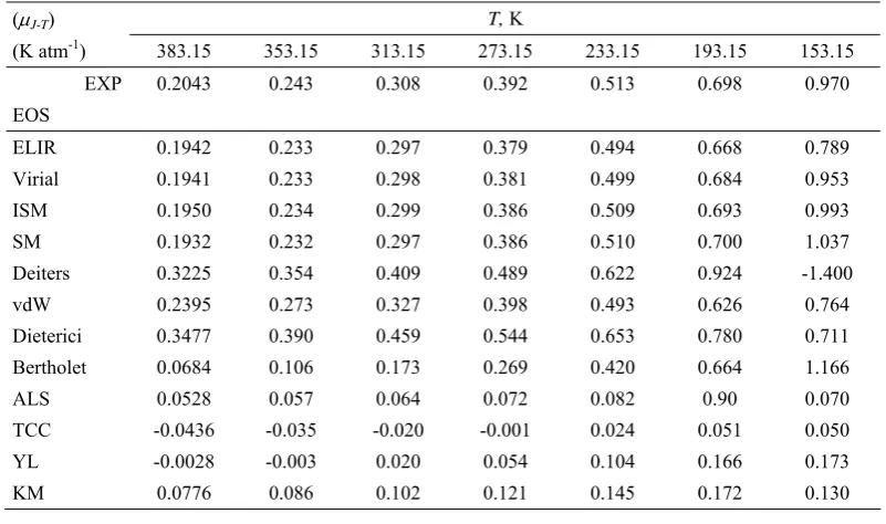
We have calculated μJ-T of argon for the temperature range of 153. 15-383.15 K at 40 atm, the experimental values of cp are taken from [15]. The results are shown in Table 2 and are compared with the experimental data [16]. This table shows that four equations of state, namely the Virial, SM, ISM, ELIR give a better result than the others. The van der Waals type equations of state predict μJ-T with a very large deviation from the experiment. The Dieterici, Deiters, Bertholet and van der Waals equations of state have also deviations, which are more significant for Deiters and Bertholet at high temperatures. However, these equations of state give better results than van der Waals type equations of state. In this way, we select the more accurate equations of state, namely the Virial, SM, ISM, and ELIR and examine their validity for different isobars.
Figures 2 and 3 show the results of μJ-T for Ar at 160 and 200 atm obtained using four selected equations of state. Even though these equations of state are in agreement with the experimental data at high temperatures, the Virial EOS shows a large deviation at low temperatures, at which it diverges. However, we
have used the Virial, ELIR, SM, and ISM, using Boushehri and Mason Correlation [17], to calculate μJ-T for different compounds such as C2H6 [18], C3H8 [19],
CO2 [20], and C7H8 [8], for which the results are shown
in Figures 4-7. Figure 4 shows the comparison between the experimental data of μJ-T for CO2 with those
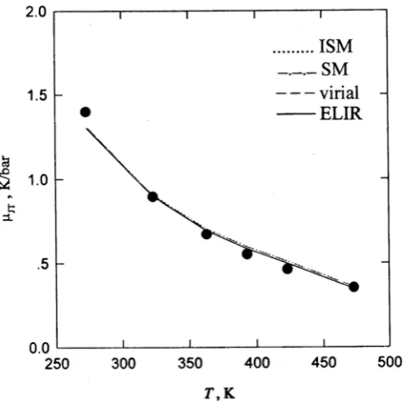
calculated from four selected equations of state in terms of temperature at 15 bar. As it is clear all four equations of state agree with the experimental data. Figure 5 shows prediction of the ISM, Virial, and ELIR for toluene for the temperature range of (530-600 K) at 20 bar. As shown the result of ISM is more accurate at least at high temperatures. Figure 6 shows the value of μJ-T versus pressure for 373.15 K isotherm of ethane (C2H6).
The results show that the Virial EOS is more accurate, except at high pressures. Figure 7 is prediction value of
μJ-T for propylene at 398.15 K. The results show that all three equations of state give good agreement with the experiment at low pressures.
Therefore, we may consider these four equations of state namely, ELIR, SM, ISM, and Virial to calculate
Figure 2. μJ-T versus temperature for Ar obtained by the ISM, SM, Virial and ELIR at 160 atm.
Figure 4. Comparison between the experimantal Joule-Thamson coefficient with those calculated from ISM, SM, Virial and ELIR for CO2 at 15 bar.
The results are shown in Figure 8 that reveals the Virial and ELIR can predict μJ-T with a good agreement with the experimental data. Similar calculations have been done for these refrigerants for different pressure and temperature ranges, and also for other refrigerants. The results are almost similar to those shown in Figure 8. But, when the deviation from the experimental data for Virial equation of state at high densities becomes
Figure 3. Same as Figure 2 for 200 atm.
Figure 5. Comparison of the ISM, Virial and ELIR for predicting the Joule-Thamson coefficient for toluene with the experimental data (●) at 20 bar.
Figure 6. μJ-T versus pressure at 373.15 K for C2H6 obtained
by four selected equations of state and experimental values(●).
Figure 8. The Joule-Thamson coefficient for R-22 at 5 bar(●), R-23 at 10 bar (■), and R-32 at 5 bar (▲) and the calculated values predicted by the ELIR (—) and Virial (……).
μJ-T in the entire temperature range.
Conclusion
In the present work, we have compared the validity of some different equations of state in predicting the Joule-Thomson coefficient. Our results for densities greater than the Boyle density show that the DSEOS
Figure 7. Same as Figure 4 for propylene at 398.15 K.
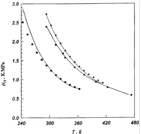
Figure 9. Joule-Thamson coefficient predicted by ELIR for R-32, R-23, R-152a and R-134a at 0.5 MPa (points are the experimental data).
the DSEOS becomes more accurate than that given by the LIR.
In the low density range, four equations of state, namely the Virial, ELIR, SM, ISM give more accurate results, therefore we recommend them for the calculation of μJ-T. Since the Joule-Thomson coefficient calculation is mainly important for refrigerants, which are mostly polar, the ELIR and Virial equations of state are appropriate for such a calculation. We have also examined these two equations for some refrigerants. The results show that the ELIR is in better agreement with the experimental data than the Virial, especially at high densities. Owing to the fact that the ELIR works up to the Boyle density (ρB is about twice of the critical density), at which the Virial equation diverges, such a result is expected. Therefore, we may conclude that by using the ELIR EOS we may obtain the most accurate value of μJ-T for refrigerants. We have also shown the predictions of the ELIR for R-134a, R-23, R-132, and R-152a, (Figure 9) which are in a good agreement with the experimental data. It is obvious from this figure that the value of μJ-T for R-152a and R-132 are the largest, in the entire range of temperature, which is in accordance with the ELIR prediction. Therefore, this EOS can be used to predict the thermodynamic state at which μJ-T has an appropriate value, without getting involved in experimental measurements.
Acknowledgements
We acknowledge the Iranian National Research Council for its financial support.
References
1. Nain, V. P. S. and Aziz, R. A. Can. J. Chem.54, 2617, (1976).
2. Edalat, M., Bozargnehri, R. and Basiri-Parsa, J. Iran. J. Chem. & Chem. Eng. 11, 43, (1992).
3. Maghari, A. and Matin, N. S. J. Chem. Eng. Jpn. 30, 520, (1997).
4. Gine, R. D. and Pravsnitze, J. M. Cryogenic, 6, 324, (1966).
5. Parsafar, G. A. and Mason, E. A. J. Phys. Chem. 97, 9084, (1993).
6. Parsafar, G. A., Farzi, N., and Najafi, B. Int. J. Thermophys. 18, 1197, (1997).
7. Alavi, S., Parsafar, G. A. and Najafi, B. Int. J. Thermophys. 16, 1421, (1995).
8. Goodwin, R. D. J. Phys. Chem. Ref. Data, 18, 1565, (1989).
9. Najafi, B. and Parsafar, G. A. J. Sci. I. R. Iran,8, 236, (1997).
10. Deiters, U. Chem. Eng. Sci. 36, 1139, (1981).
11. Song, Y. and Mason, E. A. J. Chem. Phys. 91, 7840, (1989).
12. Song, Y. and Mason, E. A. Fluid Phase Equilib. 75, 105, (1992).
13. Ihm, G., Song, Y. and Mason, E. A. J. Chem. Phys. 94, 3839, (1991).
14. Ihm, G., Song, Y. and Mason, E. A. Fluid Phase Equilib. 75, 117, (1992).
15. Stewrt, R. B. and Jacobsen, R. T., J. Phys. Chem. Ref. Data, 18, 639, (1989).
16. Strackey, J. P. and Bennett, C. O. AICHE. Journal, 20, 803, (1979).
17. Boushehri, A. and Mason, E. A. Int. J. Thermophys., 14, 685, (1993).
18. Bier, K., Kunze, J. and Maurer, G. J. Chem. Thermodyn. 8, 857, (1979).
19. Bier, K., Ernst, G. Kunze, J. and Maurer, G. J. Chem. Thermodyn. 6, 1039, (1974).
20. Bender, R., Bier, K. and Maurer, G. Ber. Bunsenger, Phys. Chem. 85, 778, (1981).
21. Ihm, G., Song, Y., and Mason, E. A. Mol. Phys., 75, 197, (1992).
22. Bier, K., Maurer, G. and Sand, H. Ber. Bunsenger.Phys. Chem. 84, 430, (1980).
23. Rasskazov, D. S., Kryvkarl, A. Tr. Mosk. Energ. Inst. 179, 108, (1974).
24. Tillner-Roth, R. and Yokozeki, A. J. Phys. Chem. Ref. Data, 26, 1237, (1997).