Load-Frequency Control in a Deregulated Environment Based
on Bisection Search
F. Daneshfar* and E. Hosseini**
Abstract: Recently several robust control designs have been proposed to the
Load-Frequency Control (LFC) problem. However, the importance and difficulties in the selection of weighting functions of these approaches and the pole-zero cancellation phenomenon associated with it produces closed loop poles. Also the order of robust controllers is as high as the plant. This gives rise to complex structure of such controllers and reduces their applicability in industry. In addition conventional LFC systems that use classical or trial-and-error approaches to tune the PI controller parameters are more difficult and time-consuming to design. In this paper, a bisection search method is proposed to design well-tuned PI controller in a restructured power system based on the bilateral policy scheme. The new optimized solution has been applied to a 3-area restructured power system with possible contracted scenarios and the results evaluation shows the proposed method achieves good performance compared with recently powerful robust controllers.
Keywords: Bisection Search, Deregulated Environment, Load-Frequency Control.
1 Introduction1
One of the important power system control problems for which a lot of studies have been made is load–frequency control (LFC) [1-3].
The main goal of LFC is to maintain zero steady state errors for frequency deviation and good tracking load demands in a multi-area power system, it is also treated as an ancillary service essential for maintaining the electrical system reliability at an adequate level [4].
However, the electric power industry is in transition from large, vertically integrated utilities providing power at regulated rates to an industry that will incorporate competitive companies selling unbundled power at lower rates. Therefore in a deregulated environment, LFC acquires a fundamental role to power system control which there has been various decentralized robust and optimal control methods to provide better conditions for the electricity trading during the last two decades [5-9]. However, most of the above robust and optimal methods need some information of the system states, which are very difficult to know completely. On the other hand, the order of the robust controllers is as high as that of the
Iranian Journal of Electrical & Electronic Engineering, 2012. Paper first received 15 Jun. 2012 and in revised form 10 Dec. 2012. * The Author is with the Department of Electrical and Computer Engineering, University of Kurdistan, Sanandaj, PO Box 416, Kurdistan, Iran.
E-mail: [email protected]
** The Author is with the Department of Mathematics, Tehran Payame Noor University, Iran.
plant. This gives rise to complex structure, complex state-feedback or high-order dynamic controllers and reduces their applicability [10].
Then despite the potential of robust control techniques with different structures, they are not practical for industry practices and power system utilities prefer the online tuned PI controller’s because of the ease of tuning and the lack of assurance of the stability and easy implementation.
In this paper a new optimization method based on bisection search [11], is used for tuning of PI controller parameters. The bisection search is a very simple and rapidly converging method in mathematics. It is a root-finding approach which repeatedly bisects an interval and then selects a subinterval in which a root must lie for further processing.
The above technique, which is ideally practical for industry, has been applied to a three-control area example as a case study and has been compared with the robust ILMI based controller proposed by [9]. The results show the optimized controller guarantee the robust performance for a wide range of operating conditions as well as full-dynamic H∞ controllers.
In this paper following a brief discussion on a deregulated LFC model, an explanation on bisection based optimization method and how a load–frequency controller can work within this formulation is provided. Simulation studies are performed to illustrate the capability of the proposed control approach. The resulting controllers are shown to minimize the effect of disturbances and achieve acceptable frequency
304 Iranian Journal of Electrical & Electronic Engineering, Vol. 8, No. 4, Dec. 2012 regulation in the presence of various load change
scenarios.
2 Background
In this section, following an introduction to the traditional and a restructured power system LFC models, the proposed control strategy has been characterized.
2.1 Conventional and Generalized LFC Model Frequency changes in large-scale power systems are a direct result of the imbalance between the electrical load and the power supplied by system connected generators [12]. A change in real power demand at one point of a network is reflected throughout the system by a change in frequency. Therefore, system frequency provides a useful index to indicate system generation and load imbalance [13]. Any short term energy imbalance will result in an instantaneous change in system frequency as the disturbance is initially offset by the kinetic energy of the rotating plant. Significant loss in the generation without an adequate system response can produce extreme frequency excursions outside the working range of the plant. The control of frequency and power generation is commonly referred to LFC which is a major function of Automatic Generation Control (AGC) systems [14].
In this classical AGC system, the balance between connected areas is achieved by detecting the frequency and tie line power deviations to generate the Area Control Error (ACE) signal which is turn utilized in the PI control strategy.
However, towards the end of the twentieth century many countries sought to reduce direct government involvement in, and to increase the economic efficiency of, their electricity industries through a change in industry managements, often described as electricity industry deregulation [4].
Deregulation is the act or process of removing or reducing state regulations. It is therefore opposite of regulation, which refers to the process of the government regulating certain activities. In another word, in contrast to the traditional power system structure that the Vertically Integrated Utility (VIU) no longer exists and the generation, transmission and distribution is owned by a single entity which supplies power to the customers at regulated rates, in an open energy market, Gencos may or may not participate in the LFC task and the common objectives, i.e. restoring the frequency and the net interchanges to their desired values for each control area are remained [7].
Deregulated systems will consist of generation companies (Gencos), distribution companies (Discos), transmission companies (Transcos) and Independent System Operator (ISO) which there can be various combinations of contracts between each Disco and available Gencos [4]. On the other hand, a Disco may contract individually with Gencos for power in different
areas (It has freedom to contract with any available Genco in its own or another control area).
To understand how the bidding process and bilateral contracts in a restructured power system are implemented, the “Generation Participation Matrix (GPM)” concept based on the idea presented by [4], is used here.
GPM shows the participation factor of a Genco in the considered control areas (Discos). The rows and columns of the GPM matrix are equal to the total number of Gencos and Discos in the overall power system, respectively. It has the following structure [7],
… …
… …
(1)
In the above matrix, refers to ‘generation participation factor’ and shows the participation factor of Genco i in the load following of area j based on the appropriate contract.
Also sum of all entries in each column of the GPM matrix according to (2) is unity.
1 2
Using the GPM matrix concept, the Gencos can submit their ramp rates (Megawatts per minute) and bids to the market operator. After a bidding evaluation, those Gencos selected to provide regulation services must perform their functions according to the ramp rates approved by the responsible organization [9].
For LFC analysis and synthesis in a deregulated environment, we use the generalized dynamical model introduced in [4]. In this scheme each control area has its own AGC and is responsible for tracking its own load and honoring tie-line power exchange contracts with its neighbors.
2.2 Three-Control Area Restructured Power System Example
In this paper, to illustrate the effectiveness of proposed control design, a three-control area power system shown in Fig. 1 (same as example used by [4]) is considered as a test system.
In this model, each control area has its own Disco, two Gencos and a PI controller which is responsible for tracking its own load and honoring tie-line power exchange contracts with its neighbors. For the simulation tests, the rate limit value for each Genco is assumed 0.1, and, 1000 MW is considered as a base for the pu calculations.
Fig. 1 Three-c
2 Most of solve and som methods hav these nonlin methods to algorithm. Th and convergi rough approx mathematica function f(x) and a≤x≤b) selects a sub 2). One way that the sign [11]. In this m equation, is t bisection sea The nece related to the
Definition 1: Suppose is w complement
Fig. 2 Bisectio
control area rest
.3 Proposed nonlinear eq me of them ar ve been propo
ear equations approximate he bisection s ing method th ximation to a al technique w
) in [a ,b] (i.e. by repeatedly binterval in w y to know tha n of f(a) is di
method the un the necessary arch [11, 15].
essary definit e bisection sea
s a set then, where is th
set of .
on search.
tructured power
d Control Stra quations are
re unsolved. T sed to approx s. One of the e the root i search is a ver hat is usually solution. It is which looks , a value of x y bisects an in which a root m at a root lies i
ifferent from niqueness root condition for
ions, theorem arch are as fol
e limit points r system.
ategy very difficult Therefore sev ximate the roo e most import
is the bisect ry simple, rob used to obtai s an optimizat for a root o x such that f(x nterval (a,b) must lie (see F
in this interva the sign of f t of the nonlin r establishing
ms and examp low,
of and is t to eral ot of tant tion bust in a tion of a x)=0 and Fig. al is f(b) near the ples the Def , Def sep gua roo Th and , Pro con so sep the Th and has wa che Ex con acc giv Ex the alg con efinition 2: are separat , efinition 3: is a conn parated sets.
Also, the arantee that th ot.
eorem 1: [16] If f be a cont d
, . oof:
Since is a nnected. Now
that 0
Now let , According to parated, then e assumption.
eorem 2: [16] If be a con d is a differen s at most a ro as given by [16
Now throug eck the above
ample 1: Let
ntinuous fu cording to the
4 sin
4 sin 4
Then ven interval ac
ample 2: Consider the
0 eorem 2, f has
2.4 Bis After the ab gorithm expla ntinuous func
ted sets if,
nected set if i
following t he equation
tinuous functi 0 then
a continuous w let
0 then 0 ∞, 0 ,
o the above as is not conn Then proof is
ntinuous functi ntiable functio oot in , .
6].
h the followi theorems app unction an following eq 4 4 4 √2 2 ha ccording to th
e function , , there at most one r
section Algor bove definiti anation is as ction defined
it is not the u
theorems an 0 has
ion in closed i 0 has at l
function, then , , if there
, .
0 , 0
.
ssumptions, s nected and th s complete.
ion in closed i on in , , th The proof of
ing two exam plications,
, . Sin
nd /4
quations, √2
2 4 0
4 0
as at least on e theorem 1.
1 efore accord root in the giv
rithm Descrip ons, the bise s follow, sup on an interva
3
union of two
nd examples just a unique
interval , least a root in
n , is
e is no any
0, ∞ where
ince , are his is opposite
interval ,
hen 0
f this theorem
mples we can
nce is a
4 /4 0
0
(4)
ne root in the
1. Obviously, ding to the en interval.
ption ection search ppose f is a al . Each o s e n s e e e 0 m n a 0 e , e h a h
306 Iranian Journal of Electrical & Electronic Engineering, Vol. 8, No. 4, Dec. 2012 iteration of the bisection algorithm evaluates the
function at the midpoint /2. Based on the sign of the evaluation, either a or b is replaced by c to retain different signs on and . Explicitly, if 0 then the subinterval , is selected and
the method sets however if 0 the
subinterval , is selected and the method sets .
If , and have the same signs, the
bisection method selects the interval which produces the
smaller value for (i.e. then
otherwise ) [11].
The bisection algorithm repeats this iteration until the interval between a and b and, hence, the resolution of the root of is as small as desired.
If is the desired root resolution then the algorithm will terminated at most in | |/ iterations, or when one of the following conditions will be true [11],
1. | | which , are the
midpoints of the interval in 1 step and the midpoint of the initial interval respectively.
2. | | , which , are the
midpoints of the interval in 1 and step.
3. | | , which is a given very small and positive number in all conditions.
Then this algorithm has the following steps and following theorems,
Step1: input ,
Step 2: let /2 : print .
Step 3: if then end.
Step 4: if 0 then let else let .
Step 5: GOTO 2. Step 6: END.
Theorem 3: [15]
The bisection method is convergent in the interval
, if 0 and is continuous.
Proof:
If is the midpoint of the interval , in the th step and is the problem solution, then absolute error in the th iterations are calculated as follow,
| |
2
| | (5)
0 | |
2 As we know:
lim 0 (6)
Consequently we have:
lim 1
2 0 lim 2 0
lim | | 0 lim (7)
Therefore, the produced sequence by the bisection algorithm is finally convergent to the root of . Following examples show the applicability of the above theorems and bisection algorithm in finding function’s roots.
Example 3:
Suppose we are going to solve the following simple equation by the bisection algorithm,
1 (8)
To solve this equation firstly we manipulate it that right side be zero. Then we have,
(9) Equivalently the goal is finding the root of function: 1. Now we guess two different
numbers , so that 0. Let 0 and
1 then 1 and 1 therefore
1 1 0.
Whereas is polynomial then it is continuous in every interval of real numbers particularly in 0,1. Therefore has conditions of theorem 1 then has at least one root in 0,1.
Derivative of function is equal to:
2 1 (10)
Obviously, ’ is positive in 0,1 , therefore
’ 0 and has conditions of theorem 2 too.
Namely 0 has at most a root in 0,1.
According to the theorem 1 and 2, 0 has just one root in 0,1 . Now we can use the bisection
algorithm to find the root of 1 in
interval 0,1.
The Table 1 shows summary of the bisection method to solve this example at five iterations. According the
Table 1, root of 1 in [0 1]
approximately is equal to .5973.
Example 4:
Suppose we are going to approximate the root of following equation by the bisection algorithm until
| | 0.01.
1 0 (11)
Table 1 Bisection method iteration for Example 3
Iterations sign of
1 0 1 0.5
+
2 0.5 1 0.75 −
3 0.5 0.75 0.625 −
4 0.5 0.625 0.5625
+
5 0.5625 0.625 0.5937 +
In fact we want to find root of function
1 .
Now we guess two different numbers such as , so
that 0. Let 0 and 1 then
1 and 1 therefore 1 1 0.
Because is a polynomial, then it is continuous in every interval of real numbers particularly in 0,1. Therefore has conditions of theorem 1 then has at least one root in 0,1.
Derivative of function is equal to,
2 5 1 (12)
Obviously, is positive in 0,1 , therefore has conditions of theorem 2 too. Namely 0 has at most a root in 0,1 .
According to the theorem 1 and theorem 2,
0 has just one root in 0,1 . Now we can use the
bisection algorithm to find the root of 1 in interval 0,1.
The Table 2 shows summary of the bisection method to solve this example at five iterations.
As it is clear from the Table 2, the root of 1 in 0,1 is approximately equal to .3437.
According to the above examples, although the bisection is a slow algorithm to approximate the root of equations, however it is so simple and unlike the most of other searching methods, it is a very convergent algorithm.
Table 2 Bisection method iteration for Example 4
It. sign of | |
1 0 1 0.5 − 0.2167
2 0 0.5 0.25
+ 0.1748
3 0.25 0.5 0.375 − 0.0452
4 0.25 0.375 0.3125 + 0.0559
5 0.3125 0.375 0.3437
+ 0.0035
3 Problem Formulation
In this paper, a bisection method obtains the approximate best values of PI controller parameters. In each control area P and I parameters have been tuned according to the absolute value of Area Control Error
(| |) signal as their evaluation function ( ). The aim
of the optimization method is to tune and parameters according to gain the smallest value of the evaluation function.
Assume and are the controller parameters of control area respectively which 0 1 and
0 1; The bisection evaluation function of area
is sum of all ACE instances over simulation time based on the specified value of P and I parameters ( , ) as follow,
, ∑ , (13)
where , ∆ , ∆ , in which ∆ , is the
frequency deviation and ∆ , is the power tie line
between area and other areas.
The bisection search for and parameters is performed as following algorithm,
Step 1: Define [0 1] as lower and upper bound criterions for solution values of and parameters of area i respectively, then 0, 1 and
0, 1.
Step 2: In each iteration two different midpoints are
calculated for control area , /2
and /2 then the 3-control area
example simulation is run according to the new solutions of and , [ , ] for each area.
Step 3: After the simulation is done, next points are selected according to the bisection evaluation
function (3), if , , 0 the
subinterval , is selected and the method sets
however if , , 0 the
subinterval , is selected and the method sets then go to the Step 2 to run the next iteration. The procedure is terminated when ,
0.001. In this case , is an optimal value for
and parameters of area .
4 Experiments
In order to demonstrate the effectiveness of the proposed strategy, it is examined in the presence of a sequence of step load changes for the various possible scenarios of bilateral contracts and load disturbances. In these simulations, the proposed optimization technique were applied to the controller of the 3-control area power system described in Background Section and the performance of it is compared with the performance of the ILMI robust controller introduced in [4].
4.1 Case Study 1: Poolco-Based Transactions The first test case study is based on the possible contracts under practical operating conditions and large load demands (a step increase in demand) by Discos of
area 1, 2, and 3 as 100 ,
70 , 60 .
A case of Poolco based contracts between Discos and available Gencos is simulated based on the following GPM. In this scenario Gencos participate only in load following control of their areas.
0.5 0 0
0.5 0 0
0 0.5 0
0 0.5 0
0 0 0.5
0 0 0.5
(14)
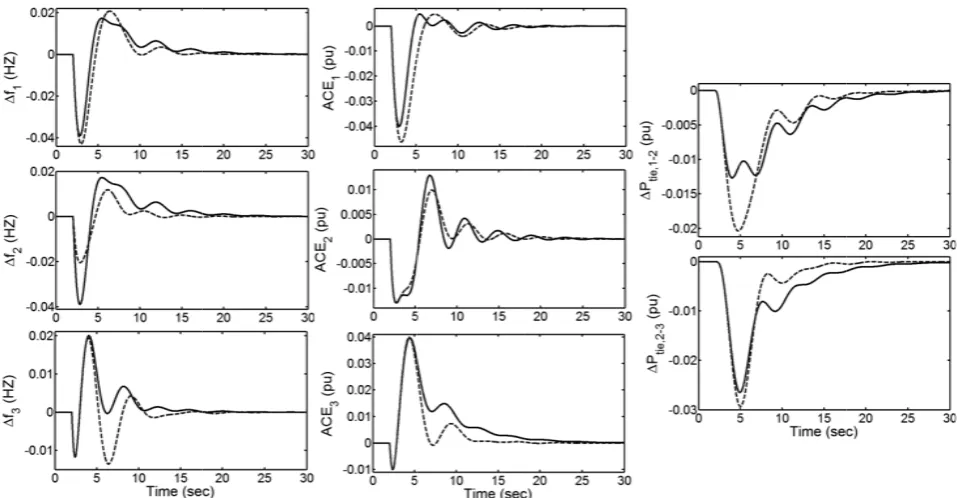
308 Frequenc and actual t loop system is used for th for ILMI bas
As shown area control are quickly overshoots. S the scheduled is zero as we
4.2 Cas
In this ca Then conside i.e.
100 .
And assu contract with according to 0 0 0. All Genc loop respons The simu steady state. seen in simu solution gen method, the
Fig. 3 Power s
cy deviation ( tie-line power are shown in he current sol sed method.
n in Fig. 3, us error and fre
driven back Since there ar
d steady state ell as ILMI rob
e Study 2: Co Bilateral-Bas ase the transac
er larger dem 100
ume Discos h h any Gencos the following 0.25 0.25 0.5 0 0 0.25 .25 0.25 0 0.25
0 0 0
cos participate ses are shown ulation results It is worth no lation results nerated signal
frequency d
system response
I ), area con r flow (
Fig. 3. In this lution and da
sing the propo equency devia k to zero a re no contract e power flow bust controller
ombination o sed Transact ction is based o mands by Disc
, 1
have the free in their areas g GPM, 0 0 0.75 0 0 0.25
e in the LFC t in Fig. 4. s show the sam oting that the
between ILM ls. Also usin deviation of a
e to case study
Iranian Journ ntrol error (
) for the clo figure, solid l shed line is u
osed method, ation of all ar and have sm ts between are over the tie-li r.
of Poolco and ions
on free contra o 2 and Disco
100 ,
edom to hav s and other ar
(
task. The clos
me values in small differen MI and the curr ng the propo all areas quic
1: Solid line (p
nal of Electrica ) osed line used the reas mall eas, ines d acts. o 3, ve a reas 15) sed-the nces rent osed ckly dri too per ran bou unc are 5 pow dem flu con sim rob con pos non ind sol pos Fo rob val per con rel ILM proposed strateg
al & Electron iven back to z o.
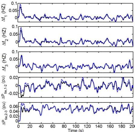
The purpos rformance of ndom load dis
Consider the unded rando contracted loc ea as follow:
50 The correspo wer changes monstrates tha uctuations, ef ntrollers. The above si mple and eas bust performa ntroller techn ssible contrac nlinearities. F dependency a lution for a ssible bilatera r more inv bustness of th
lue of rformance in ntrol scheme a
As shown in atively better MI based desi
gy), Dashed line
nic Engineerin zero and has
4.3 Case se of this proposed con turbances. e GPM of sc om load ch
cal demand,
50 onded frequen
are shown at the designe ffectively as
imulation resu sy optimizatio ance as well nique with c cted scenarios Furthermore th
and simple s wide range al contract sce vestigation a e proposed co over three ndex for com and ILMI desi n Table 3 the r performance
ign.
e (ILMI based a
ng, Vol. 8, No. a good dyna
Study 3 scenario is ntrollers agai
enario 2 agai hanges (Fig. is applied to
ncy deviation in Fig. 6. ed controllers t
s well as
ults show that on method a
as powerful complex struc s in the presen he higher flex structure of t of load distu narios are inv and to dem ontrol strategy e minutes is mparison of t
ign.
e current solu e than the co
approach).
4, Dec. 2012 amic response
to test the nst large and
in. Assume a 5) as an each control
(16) ns and tie-line This figure track the load ILMI based
t the proposed achieve good ILMI robust cture for the nce of system xibility, model the proposed urbances and vestigated. monstrate the
y, the average s used as a the proposed
ution presents mplex robust 2 e e d a n l e e d d d d t e m l d d e e a d s t
Fig. 4 Power s
Table 3 Perfor M
Proposed ILMI-ba
5 Conclusi In this p technique for has been pro proposed m converging t area power s this new sc frequency, t interchange p values. Ther
Fig. 5 Random
system response
rmance Evaluat
Method
d Controller sed
ion
paper, an eas r the LFC des oposed in a de method is a
technique and system with d
heme, in add the AGC sys power with n refore, a des
m load changes.
e to case study
tion.
Case S
|ACE1|avg |ACE 0.0013 0.00 0.0025 0.00
sy implement sign, using the eregulated po a very simp d was applie different possi dition to the stem should neighboring ar sirable AGC
.
2: Solid line (p
Study 1
E2|avg |ACE3|av 024 0.0044 025 0.0023
ted optimizat e bisection sea ower system. T ple, robust
d to a 3-con ible scenarios regulating a control the reas at schedu performance
proposed strateg
Ca
vg |ACE1|avg 0.0034 0.0020
tion arch The and ntrol s. In area net uled e is
ach min pow cha
Fig
(pr
gy), Dashed line
ase Study 2
|ACE2|avg |AC 0.0032 0.00 0.0038 0.00
hieved by e nimize frequ wer flows. T anges by se
g. 6 Power sy
oposed strategy
e (ILMI based a
CE3|avg |ACE1|av 022 0.0063 031 0.0098
effective adj uency deviati The AGC sy ending signal
stem response y), Dashed line
approach).
Case Study 3
vg |ACE2|avg 0.0110 0.0130
usting of g ion and regu ystem realize
ls to the u
to case study (ILMI based).
|ACE3|avg 0.0126 0.0118
generation to ulate tie-line es generation under control
y 3: Solid line o e n l
e
310 Iranian Journal of Electrical & Electronic Engineering, Vol. 8, No. 4, Dec. 2012 generating units. The simulation results in the new
model, show that it presents a desirable performance under a wide range of load changes specially compare with robust controllers. Moreover, this newly developed solution has a simple structure, and is fairly easy to implement in comparison to other controllers, which can be useful for the real world complex power systems.
Acknowledgment
The authors wish to thank Dr. H. Bevrani for his help in providing the 3-control area power system model.
References
[1] Ibraheem, Kumar P. and Kothari P., “Recent philosophies of automatic generation control strategies in power systems”, IEEE Trans. on Power Systems, Vol. 20, No. 1, pp. 346-357, 2005.
[2] Kothari ML., Nanda J., Kothari D. P. and Das D., “Discrete mode AGC of a two area reheat thermal system with new ACE”, IEEE Trans. on Power Systems, Vol. 4, pp. 730-738, 1989.
[3] Shoults R. R. and Jativa J. A., “Multi area adaptive LFC developed for a comprehensive AGC simulator”, IEEE Trans. on Power Systems, Vol. 8, pp. 541-547, 1991.
[4] Bevrani H., Frequency Response Characteristics and Dynamic Performance, Robust power system frequency control, 1st edn, Springer Press, 2009,
pp. 49-59.
[5] Ishi T., Shirai G. and Fujita G., “Decentralized load frequency based on H‐inf control”, Electr. Eng. Jpn., Vol. 136, No. 3, pp. 28-38, 2001. [6] Kazemi M. H., Karrari M. and Menhaj M. B.,
“Decentralized robust adaptive‐output feedback controller for power system load frequency control”, Electr. Eng. J., Vol. 84, pp. 75-83, 2002. [7] Liu F., Song Y. H., Ma J. and Lu Q., “Optimal load frequency control in the restructured power systems”, IEE Proceedings Generation Transmission & Distribution, Vol. 15, No. 1, pp. 87-95, 2003.
[8] Bevrani H. and Hiyama T., “Robust
load‐frequency regulation: a real‐time laboratory experiment”, Optimal Control Applications and Methods, Vol. 28, No. 6, pp. 419‐433, 2007. [9] Bevrani H., Mitani Y. and Tsuji K., “Robust
decentralised load‐frequency control using an iterative linear matrix inequalities algorithm”,
IEE Proc. Gener. Transm. Distrib. Vol. 3, No. 151, pp. 347‐354, 2004.
[10] Shayeghi H., Shayanfar H. A. and Jalili A., “Multi-stage fuzzy PID power system automatic generation controller in deregulated environments”, Energy Conversion and Management, Vol. 47, No. 18-19, pp. 2829-2845, 2006.
[11] Hamming R. W., Numerical methods for scientists and engineers. Mc Graw-Hill, New York. 1962.
[12] Daneshfar F. and Bevrani H., “Load-Frequency Control: A GA-based Multi-agent Reinforcement Learning”, IET Generation, Transmission & Distribution, Vol. 4, No. 1, pp. 13-26, 2010. [13] Jaleeli N., Ewart D. N. and Fink L. H.,
“Understanding automatic generation control”, IEEE Trans. Power Syst. Vol. 7, No. 3, pp. 1106‐1112, 1992.
[14] Hiyama T., “Design of decentralised load‐frequency regulators for interconnected power systems”, IEE Proc. C Gener. Transm. Distrib. Vol. 129, pp. 17–23, 1982.
[15] Froberg, CE., Numerical mathematics, theory and computer applications. The Benjamin Publishing Company, MA. 1985.
[16] Rudin, W., Principles of mathematical analysis. 3rd ed. McGraw-Hill, New York. 1976.
Fatemeh Daneshfar received B.Sc.
degree in Electrical and Computer Engineering from University of Tehran, Tehran, Iran, in 2003 and M.Sc. degree in Artificial Intelligence at the Department of Electrical and Computer Engineering in University of Kurdistan in 2009. Her research interest is on multi-agent systems and intelligent solutions for control systems.
Eghbal Hosseini received B.Sc.
degree in Applied Mathematics from University of Razi, Kermanshah, Iran, in 2005 and M.Sc. degree in Operation Research at the Department of Science in University of Kurdistan in 2007. He is Ph.D. student in Department of Mathematics, Tehran Payame Noor University, Iran now. His research interest is on bi-level programming problem and optimization.