Optimal Link-Disjoint Node-“Somewhat Disjoint”
Paths
Jose Yallouz
∗, Ori Rottenstreich
†, P´eter Babarczi
‡, Avi Mendelson
∗, Ariel Orda
∗∗Department of Electrical Engineering, Technion, Israel Institute of Technology †Department of Computer Science, Princeton University
‡MTA-BME Future Internet Research Group, Budapest University of Technology and Economics (BME) ∗[email protected], †[email protected], ‡[email protected], ∗{mendlson, ariel}@ee.technion.ac.il
Abstract—Network survivability has been recognized as an issue of major importance in terms of security, stability and prosperity. A crucial research problem in this context is the identification of suitable pairs of disjoint paths. Here, “disjointness” can be considered in terms of either nodes or links. Accordingly, several studies have focused on finding pairs of either link or node disjoint paths with a minimum sum of link weights. In this study, we investigate the gap between the optimal node-disjoint and link-disjoint solutions. Specifically, we formalize several optimization problems that aim at finding minimum-weight link-disjoint paths while restricting the number of its common nodes. We establish that some of these variants are computationally intractable, while for other variants we establish polynomial-time algorithmic solutions. Finally, through extensive simulations, we show that, by allowing link-disjoint paths share a few common nodes, a major improvement is obtained in terms of the quality (i.e., total weight) of the solution.
I. INTRODUCTION
A. Background
Survivability, i.e. the capability of the network to maintain service continuity in the presence of failures, has been con-sidered as a major challenge for the networking community. A fundamental problem in this context is the identification of a pair of disjoint paths, thus providing protection against a single failure in the network. Usually, such a pair of paths needs to satisfy some quality (a.k.a. “Quality of Service -QoS”) requirement, which is typically quantified by the sum of some link weights. Accordingly, several studies have proposed algorithmic schemes for finding a fully disjoint pair of paths between a source and a destination that minimize the sum of the link weights [1], [2]. “Disjointness” can be considered either in terms of links or nodes. We note that a link-disjoint pair of paths might contain severalcommon nodes, whereas the node-disjoint solution is a special case of link-node-disjointness with no common nodes.
From a practical perspective, common nodes along an es-tablished link-disjoint pair of paths might have either (or both) beneficial or detrimental implications. For instance, in cases that the recovery time is critical, the traffic might be retransmitted from the closest common node to the faulty link rather than from the source. However, in case of faulty nodes, a common node becomes asingle point of failure. Accordingly,
the detrimental and beneficial effects of common nodes can be considered together by allowing (or, alternatively, requiring) that the pair of link-disjoint paths would share a bounded number of common nodes.
In this study, we aim to investigate the whole spectrum of minimum-weight link-disjoint solutions while allowing a certain (bounded) number of common nodes. Accordingly, in Section II, we formalize several optimization problems that aim to find a link-disjoint pair of paths with minimum weight with a restriction on the number of its common nodes. Specifically, we define three problem variants where the restriction on the common nodes constitutes, respectively, an upper-bound, a tight-bound or a lower-bound. We begin by establishing the NP-Hardness of the lower-bound and the tight-bound problems, in Section III. For the upper-bound problem, in Section IV, we provide an optimal polynomial-time algorithm. Then, we con-tinue to establish a polynomial-time solution for the problem variant in which the number of common nodes is considered as a secondary metric, i.e. finding a minimum weight link-disjoint pair of paths with maximum number of common nodes. In Section V, we propose a polynomial-time solution for the three specified problems for the case of Directed Acyclic Graphs (DAGs). Finally, in Section VI, by employing the established algorithmic schemes, we are able to study the gap between the optimal node-disjoint and the optimal link-disjoint solution through extensive simulations.
B. Related Work
polynomial-time by the well-known Suurballe’s algorithm [1], [2]. However, other objective functions might be considered as well. In [5], the problem of finding link-disjoint paths minimizing the weight of the longest path was proved to be NP-Hard, while Suurballe’s algorithm provides a2-approximation. In [6], the minimization of the shorter path was addressed and proved to be strongly NP-Hard. Next, in [7], the problem of finding a link-disjoint pair of paths that minimizes the total cost of the paths under a constraint imposed by a second weight metric has been considered. This problem was proved to be NP-Hard and a bi-criteria O(1 +1r,1 +r)approximation for anyr≥0was proposed. Recently, in [8], an improved constant approximation ratio of(1,2) was achieved.
The present study is somehow related to the concept of tunable survivabilitywhich offers a milder and more flexible approach to the rigid requirement of link-disjoint paths by also considering paths containing common links [9]–[11]. These works first focused on “bottleneck” QoS [9] metrics, then con-sidered the harder class of “additive” QoS [10], while extended in the context of broadcasting through spanning trees [11].
II. MODELFORMULATION
Anetworkis represented by a directed graphG(V, E), where V is the set of nodes andE is the set of links. We denote the size of these sets as|V|=N and|E|=M, respectively. Each link e ∈E is assigned with a positive weight we ∈ R+ that represents an additive QoS target, e.g. cost or delay. Apathis a finite sequence (ordered set) of nodesπ=< s0, s1, ..., sh> such that si ∈ V (for i ∈ [0, h]) and (si, si+1) ∈ E (for
i∈[0, h−1]). A path issimpleif its nodes are distinct. Unless explicitly stated, the termpathis used for a simple path. Along the paper, a link and a path between nodesuandvcan be also represented byu→v andu v, respectively.
A common approach for failure protection is the usage of a pair of (fully) link-disjoint paths between given source and destination nodes.
Definition 2.1:(Link-disjoint Path Pair) Given are a network G(V, E), a source nodes∈V and a destination nodet∈V. A link-disjoint path-pair(π1, π2)is a pair of paths between these
nodes with no common links.
While two paths must be link-disjoint to guarantee surviving any single link failure, they still might share common nodes.
Definition 2.2: (Common Node) Given a link-disjoint path-pair(π1, π2) between a source nodes∈V and a destination
nodet∈V, acommon nodeof(π1, π2)is a node, other than the
source and destination, that belongs to both paths, i.e. a node in{v∈V \ {s, t}|v∈π1andv∈π2}. We defineC(π1, π2)as
the number of common nodes of(π1, π2).
Accordingly, anode-disjoint path-pair(π1, π2)is a pair of
link-disjoint paths between these nodes with no common nodes, i.e. C(π1, π2) = 0.
Often, the weight of a path is defined as the sum of its link weights [12]. This can describe, for instance, the total cost or delay along the path. Generally, we would prefer paths with smaller weights. Since a link-disjoint path-pair is composed of two paths, there are several possibilities to define its weight
based on its link weights. We adopt the classical metric which considers the aggregate (total) weight of the two paths (e.g., [1], [2], [13]). This metric accounts for the “average quality” of the paths, and is also suitable in cases where the incorporation of each link in either path incurs some “cost” (e.g., maintenance cost).
Definition 2.3:Given a network G(V, E)and a link-disjoint path-pair(π1, π2), itsweight W(π1, π2)is defined as the sum
of weights of the links of its two paths, i.e., W(π1, π2) = P
e∈π1∪π2we = P
e∈π1we + P
e∈π2we. Accordingly, we define a weight-shortest link-disjoint path-pair between two nodesu∈V andv∈V as a link-disjoint path-pair inG(V, E) with minimum weight betweenuandv.
Among the different weight-shortest link-disjoint path-pairs, we might have to cope with different restrictions on the number of common nodes, resulting in the following optimization problems.
Problem 2.1: Minimum Weight Link Disjoint Paths re-stricted Upper Bound Common Nodes (MWLD-Upper-BCN) Problem:Given are a networkG(V, E), a source nodes∈V, a destination nodet∈V and an integerk. Find a link-disjoint path-pair(π1, π2)such that:
min W(π1, π2)
s.t. C(π1, π2)≤k.
Problem 2.2: Minimum Weight Link Disjoint Paths re-stricted Tight Bound Common Nodes (MWLD-Tight-BCN) Problem:Given are a networkG(V, E), a source nodes∈V, a destination nodet∈V and an integerk. Find a link-disjoint path-pair(π1, π2)such that:
min W(π1, π2)
s.t. C(π1, π2) =k.
Problem 2.3: Minimum Weight Link Disjoint Paths re-stricted Lower Bound Common Nodes (MWLD-Lower-BCN) Problem:Given are a networkG(V, E), a source nodes∈V, a destination nodet∈V and an integerk. Find a link-disjoint path-pair(π1, π2)such that:
min W(π1, π2)
s.t. C(π1, π2)≥k.
In the sequel, we will prove that the MWLD-Tight-BCN and the MWLD-Lower-BCN problem versions are NP-Hard, while for the MWLD-Upper-BCN problem we shall establish a polynomial-time solution.
III. MWLD PROBLEMSHARDNESS
In this section, we will prove the complexity of two problem variants, namely MWLD-Tight-BCN and MWLD-Lower-BCN.
A. MWLD-Tight-BCN Intractability
pathsΠ1andΠ2between(s1, t1)and(s2, t2), respectively. The
complexity of different versions of the problem (Gis directed or undirected, and Π1 and Π2 are link- or node-disjoint) has
been investigated in [15]. Shiloach presented a polynomial-time solution for the 2-(node-)disjoint paths problem in undirected graphs [16], while Tholey [17] further improved the time complexity of this algorithm. However, the 2-Disjoint Paths Problem remains NP-complete in directed graphs [14] for both the link- and disjoint case [17]. We will refer to the node-disjoint problem in directed graphs as 2-NDPP.
We proceed to define a decision version of the MWLD-Tight-BCN problem and the 2-NDPP problem, respectively.
• Given are a directed network G(V, E) with positive link weights we ∈ R+, two distinct nodes s, t, a positive integer k and a positive value l. Is there a link-disjoint path-pair(π1, π2)betweensandtsuch thatC(π1, π2) =k
andW(π1, π2)≤l?
• Given are a directed network G(V, E) and four distinct nodess1, t1, s2andt2. Are there2node-disjoint pathsΠ1
andΠ2between (s1, t1)and(s2, t2), respectively?
Next, we show that the MWLD-Tight-BCN problem is NP-complete even for k= 1.
Theorem 3.1: The MWLD-Tight-BCN problem for C(π1, π2) = 1 is NP-complete.
Proof: Clearly, MWLD-Tight-BCN is in NP, since for a given link-disjoint path-pair (π1, π2), we can polynomially
check whether W(π1, π2)≤l andC(π1, π2) = 1by summing
its link weights and counting its common nodes, respectively. We proceed to prove that the MWLD-Tight-BCN problem for C(π1, π2) = 1is NP-Hard by providing a polynomial-time
reduction from the 2-NDPP (NP-Hard) problem, i.e.2-NDPP p MWLD-Tight-BCN. Assume we are given an instance of the 2-NDPP problem, that is, a directed graph G(V, E) and four distinct nodes s1, t1, s2 andt2. In the polynomial-time
reduction, we create a directed graphG1(V1, E1), whereV1=
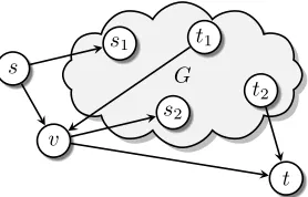
V ∪ {s, t, v}, wheresandt denote the source and destination node of the MWLD-Tight-BCN problem, respectively, while E1=E∪ {(s, s1),(s, v),(t1, v),(v, s2),(v, t),(t2, t)}. We set
∀e∈E1 : we= 1,l =Pe∈E1we andk= 1. This auxiliary graph G1(V1, E1)is illustrated in Fig. 1.
Next, we will demonstrate that the MWLD-Tight-BCN prob-lem in G1 is solvable, i.e., there is a link-disjoint path-pair
(π1, π2) from s to t with exactly one node in common and
W(π1, π2)≤l iff 2-NDPP is solvable in G.
(⇒) First, note that the single common node in G1 for the
MWLD-Tight-BCN problem must be v. This is because if π1
and π2 have the single common node w inside G, i.e., π1 =
s → s1 w t2 → t and π2 = s → v → s2 w
t1 →v →t, thenπ2 is a non-simple path. Furthermore, note
that the segments Π1 =s1 t1 and Π2 =s2 t2 must be
part of the MWLD-Tight-BCN solution, as otherwise π1 and
π2 do not have a node in common (i.e., π1=s→v→tand
π2=s→s1 t2→t).
Therefore, in G1there are two possible MWLD-Tight-BCN
solutions. In the first case, the node-disjoint paths of 2-NDPP
G s
v s1
s2
t2
t1
[image:3.612.372.511.57.146.2]t
Fig. 1. Polynomial-time reduction of2-NDPP to MWLD-Tight-BCN.
Π1 =s1 t1 and Π2 =s2 t2 are part of the same
link-disjoint path of MWLD-Tight-BCN, wlog π1 = s → s1
t1 →v →s2 t2 →t and π2 =s→v →t with common
nodev. As bothπ1andπ2are link-disjoint simple paths in the
MWLD-Tight-BCN solution, there are no repeating nodes in π1, i.e., its path segments Π1 andΠ2 are node-disjoint, thus,
2-NDPP is solved in G. In the second case, the link-disjoint paths are π1 = s → s1 t1 → v → t and π2 = s →
v → s2 t2 → t with a single common node at v. As
v is already a common node, the two paths cannot have other common nodes inG, i.e., theΠ1=s1 t1segment ofπ1and
theΠ2=s2 t2 segment ofπ2are node-disjoint, and again,
2-NDPP is solved. Both solutions clearly haveW(π1, π2)≤l.
(⇐) Given a 2-NDPP solution with node-disjoint simple pathsΠ1 andΠ2, we can easily construct link-disjoint simple
pathsπ1 andπ2 for MWLD-Tight-BCN with common nodev
and W(π1, π2) ≤l, e.g., π1 =s → s1 t1 → v → t and
π2 = s → v → s2 t2 → t. Thus, we conclude the proof
that the two problems are solvable at the same time.
Note that, for an arbitraryC(π1, π2) =kgraph Gk(Vk, Ek) is constructed in the same way asG1(V1, E1)with the
exten-sion that now we replace t with a chain of k nodes which π1 and π2 must have in common, i.e., Vk = {V1 \ t ∪
v1, v2, . . . , vk−1, vk =t}with duplicated linkse1i = (vi, vi+1),
e2
i = (vi, vi+1), i = 1, . . . , k − 1 between them. Hence,
Ek ={E1\(v, t),(t2, t) ∪ (v, v1),(t2, v1),∀i : e1i, e2i}. The link weights andl are defined similarly as in G1.
Corollary 3.1: (By the reasoning of Theorem 3.1) The NP-completeness of MWLD-Tight-BCN forC(π1, π2) =kfollows
inGk(Vk, Ek).
B. MWLD-Lower-BCN Intractability
• Given are a directed network G(V, E) with positive link weights we ∈ R+, two distinct nodes s, t, a positive integer k and a positive value l. Is there a link-disjoint path-pair(π1, π2)betweensandtsuch thatC(π1, π2)≥k
andW(π1, π2)≤l?
• Given are a directed networkG(V, E), two distinct nodes
s, t, and a positive integer p. Is there a simple path π betweensandtsuch thatL(π)≥p?
Next, we show that the MWLD-Lower-BCN problem is NP-complete.
Theorem 3.2: The MWLD-Lower-BCN problem is NP-complete.
Proof: Clearly, MWLD-Lower-BCN is in NP, since for a given link-disjoint path-pair (π1, π2), we can polynomially
check whether W(π1, π2)≤l andC(π1, π2)≥kby summing
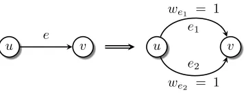
its link weights and counting its common nodes, respectively. We proceed to prove that the MWLD-Lower-BCN problem is NP-Hard by providing a polynomial-time reduction from the Longest-Path (NP-Hard) problem, i.e. Longest-Path p MWLD-Lower-BCN. Assume we are given an instance of the Longest-Path problem, that is, a directed graph G(V, E), two distinct nodes s, t, and positive integer p. In the polynomial-time reduction, we create a directed graphGD(VD, ED), where VD = V, while each link e ∈ E is duplicated in ED, i.e. ED ={e1 = (u, v), e2 = (u, v)|e= (u, v)∈ E}. This
trans-formation is illustrated in Fig. 2. We set ∀e∈ED :we = 1, l=P
e∈EDweandk=p−1.
Next, we will demonstrate that the MWLD-Lower-BCN problem is solvable – i.e., there is a link-disjoint path-pair (π1, π2) froms tot whereC(π1, π2)≥k andW(π1, π2)≤l
iff Longest-Path problem is solvable in G.
(⇒) Consider a link disjoint path-pair (π1, π2) solution for
the MWLD-Lower-BCN. Clearly, every (π1, π2) solution has
W(π1, π2)≤l =Pe∈EDwe. Moreover, (π1, π2)has at least
k common nodes, i.e. C(π1, π2)≥k, therefore, both paths π1
and π2 have at least k+ 1 links. Note that the nodes sand t
are excluded from the common nodes set by definition. Without loss of generality, consider π1 inGD, its equivalent links in G provide a pathπinGsuch thatL(π)≥k+ 1 =psolving the Longest-Path problem.
(⇐) Given a Longest-Path problem solution πinGwith at least plinks, we can easily construct link-disjoint simple paths π1 and π2 for MWLD-Lower-BCN with p−1 common node
andW(π1, π2)≤l=Pe∈EDweby considering the duplicated
links at GD for each of the disjoint paths. In other words, for each e ∈ π which represents e1, e2 ∈ ED, we construct (π1, π2)such thate1∈π1 ande2∈π2. This (π1, π2)solution
solves the (π1, π2) problem sinceC(π1, π2)≥k=p−1 and
W(π1, π2)≤l=Pe∈EDwe.
Note that the MWLD-Lower-BCN problem remains NP-Hard even for a simple (without parallel links) graph. It can be done by a simple manipulation in the reduction, in which an intermediate node is added for each duplicated link (remaining the instance graph of the reduction GD simple). This manipulation can be applied for MWLD-Tight-BCN as
u e v u v
e1
e2
we1 = 1
[image:4.612.352.530.58.126.2]we2 = 1
Fig. 2. Polynomial-time reduction of linksEof Longest-Path to the duplicated linksEDof MWLD-Lower-BCN.
well. Moreover, both MWLD-Lower-BCN and MWLD-Tight-BCN problems remain NP-Hard even for the unweighted graph version since their NP-Hardness proofs hold for the particular case where we= 1for all links.
IV. ALGORITHMICSCHEMES
In the previous section, we proved that two of the previously formulated optimization problems, namely MWLD-Tight-BCN and MWLD-Lower-BCN, are NP-Hard, leaving hope for an efficient solution for the third problem variant, namely MWLD-Upper-BCN problem. Indeed, in this section, we shall provide a polynomial algorithmic scheme for the MWLD-Upper-BCN problem. We also suggest a solution to a new problem variant.
A. Establishing Link-Disjoint Paths solving the MWLD-Upper-BCN Problem
We proceed to establish an exact solution of polynomial complexity for the MWLD-Upper-BCN problem.
The solution approach is based on a graph transformation that reduces our problem to a standardL-Link Shortest Path (L-LSP) problem. We recall thatL-LSP is the problem of finding a weight shortest path with at most Llinks.
Definition 4.1: L-Link Shortest Path (L-LSP) Problem: Given is a network G(V, E) where each link e ∈ E is associated with a positive length we. Let L be a positive integer and s, t∈V be the source and the destination nodes, respectively. Find a weight-shortest pathπ, i.e.min P
e∈πwe, fromstot with at mostLlinks.
˜
u v˜
u v
˜
we˜=W(π1) +W(π2)
˜ e W(π1)=Pe∈π1we
W(π2)=Pe∈π2we
Fig. 3. Disjoint links transformation.
of Paths (NDSPoP) between pairs of nodes in the (original) network. The weight of each link is computed by employing any NDSP Algorithm [1], [2], [13], and is given by the weight of the NDSPoP between these two nodes, as illustrated in Fig. 3. Given the common node upper bound constraintk, the second stage calculates a weight-shortest path with at mostk+1 links betweensandtin the new auxiliary networkG( ˜˜ V ,E)˜ by applying theL-Link Bellman-Ford Algorithm whereL is set to bek+1. The Bellman-Ford Algorithm is based on a dynamic programming approach, where the distance of each node can be improved by handling all links in the graph iteratively. At iteration i of the algorithm, it outputs a shortest-weight path with at most i links. Therefore, by stopping the algorithm execution at i=k+ 1, we will have an optimal path ˜πwith at most k common nodes. The links of the optimal path π˜ represents NDSPoPs at the original network. As shall be shown, these NDSPoPs do not contain a common node (except to its source and destination). Furthermore, there is no solution to our problem if there is no feasible solution to the defined L-LSP problem. Accordingly, in the third stage, we construct the sought pair of paths of a link-disjoint path-pair solution(π1, π2)
out of the links of the BF solution. Then, the algorithm outputs the optimal solution(π1, π2).
The following theorem states the correctness of the MWLD-Upper-BCN Algorithm.
Theorem 4.1:Given are a networkG(V, E), a pair of nodess andt, and an upper bound constraint on the number of common nodes k. If there exists a link-disjoint path-pair of at most k common nodes, then the MWLD-Upper-BCN Algorithm returns a feasible weight-shortest link-disjoint path-pair that is a solution to the MWLD-Upper-BCN Problem 2.1; otherwise, the algorithm fails.
Proof:In order to establish the proof, we begin by observ-ing that the structure of any link-disjoint path-pair (π1, π2)is
composed of node-disjoint subpath-pairs between its common nodes. For a given link-disjoint path-pair(π1, π2), we define the
common node set as the ordered set of common nodes along the paths π1 and π2 including s and t, i.e. {c ∈ V|c ∈ π1
and c ∈ π2}. We note that the common nodes must appear
in the same order in the two paths (assuming they are simple). Otherwise, if for instance for two common nodesc1, c2we have
π1=s c1 c2 t, π2 =s c2 c1 t, they can be
replaced by two paths s c1 t, s c2 t, obtained by
switching their subpaths while reducing the total weight and the number of common nodes.
Input:
G(V, E)- network,s- source,t - destination,we - link weight, k- common node upper bound constraint
Variables: ˜
G( ˜V ,E)˜ - auxiliary network,s˜- source,˜t- destination,w˜˜e -link weight in the auxiliary network,π˜ - BF solution
Stage1 - Auxiliary networkG( ˜˜ V ,E)˜ construction -V˜ V
foreach u∈V do foreach v∈V do
- Employ theNDSP Algorithm[2] between uandv.
if (there is a solution to the NDSP Algorithm) then
- Construct a linke˜betweenu˜ and˜v. - Assignw˜˜eto be the sum of we’s of the Node-Disjoint Shortest Pair of Paths (NDSPoP).
end end end
Stage2 - Bellman-Ford (BF) Calculation
- Given the auxiliary networkG( ˜˜ V ,E), find a shortest path˜ π˜ betweens˜and˜t with at mostk+ 1 links by employing Bellman-Ford (BF) Algorithm variant with instance <G( ˜˜ V ,E),˜ s,˜ ˜t,w˜˜e, k+ 1>
if there is no feasible solution for the BF Algorithm then
- returnFail
end else
- Let ˜πrepresent the solution of the BF Algorithm
end
Stage3- Shortest Pairs of Link-Disjoint Paths(π1, π2)
Construction
foreach ˜e∈π˜ do
- π1 contains the links of one path of the NDSPoP
represented by ˜e.
- π2 contains the links of the other path of the NDSPoP
represented by ˜e.
end
return(π1, π2)
Fig. 4. MWLD-Upper-BCN Algorithm
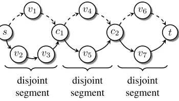
Accordingly, we define a disjoint segment ci(π1, π2)ci+1 between two sequential common nodes ci and ci+1 in the
common node set as the node-disjoint subpath-pairs ofπ1 and
π2 between ci andci+1. The above definitions are illustrated
in Fig. 5.
The weight of a disjoint segment W(ci(π1, π2)ci+1) is de-fined as the sum of all link weights in the disjoint segment, i.e. W(ci(π1, π2)ci+1) =
P
e∈ci(π1,π2)ci+1
we. Accordingly, a shortest disjoint segment is a disjoint segment ci(π1, π2)ci+1 of minimum weight among all possible disjoint pairs of paths fromci toci+1.
s v1
v2 v3
c1
v5
v4
c2
v6
v7
t
disjoint segment
disjoint segment
[image:6.612.87.262.56.155.2]disjoint segment
Fig. 5. A link-disjoint path-pair(π1, π2)illustrated in the dashed and solid
line. It contains the disjoint segmentss(π1, π2)c1,c1(π1, π2)c2,c2(π1, π2)t,
respectively, wherec1andc2 are common nodes.
MWLD-Upper-BCN Problem is such that all its disjoint seg-ments are shortest disjoint segseg-ments.
Proof:Let(π1, π2)be an optimal solution of the
MWLD-Upper-BCN Problem. We refer to the order of the disjoint seg-ments according to the order of their common nodes. Assume by contradiction the existence of a disjoint segmentc1(cπ1,cπ2)c2 with a lower weight between some common nodes c1, c2 and
consider the solution obtained by replacing the corresponding existing disjoint segment by the new one. Clearly, the weight of the solution is reduced. We need to show we can also limit the number of common nodes after the replacement. If the new segment has a node similar to some node that appears earlier in one of the two paths (necessarily not in the same segment), we can merge the latest node with such property with the similar one and eliminate the loop between them to get a path with a lower weight. Likewise, we merge the earliest node in the remaining part of the new segment that appears also in later segments. We obtain a legal solution with a reduced weight and a not larger number of common nodes in contradiction to the optimality of(π1, π2). Thus necessarily the original segment is
a shortest disjoint segment.
Lemma 4.1 justifies the construction in step1of the MWLD-Upper-BCN Algorithm (Fig. 4) in which the links in the auxiliary network G( ˜˜ V ,E)˜ are associated with the shortest disjoint segments between all pairs of nodes in the network.
We proceed to show that we can obtain a pair of simple paths from any (optimal) solution to the BF algorithm in stage2 of the MWLD-Upper-BCN Algorithm. Consider a link˜ebetween ˜
u and v˜ in the auxiliary network G( ˜˜ V ,E)˜ which represents the disjoint segment u(π1, π2)v in G. We say that two links ˜
e1 and e˜2 in the auxiliary network G( ˜˜ V ,E)˜ representing the
disjoint segments c1(π1, π2)c2 and c3(π1, π2)c4 are mutually node disjointif their corresponding segments do not have any common nodes (ignoring c1,c2,c3 andc4).
Lemma 4.2:Any optimal solution˜πof theL-LSP problem in stage2of the MWLD-Upper-BCN Algorithm (Fig. 4) is such that all its links are mutually node disjoint.
Proof: Let π˜ with k+ 1 links be the solution of the L-LSP problem in stage2of the MWLD-Upper-BCN Algorithm representing (π1, π2) in the original network. Consider some
arbitrary two links in the solution, namely s˜1 → t˜1 and
˜
s2 → t˜2 representing s1(π
1
1, π21)t1 and s2(π
2
1, π22)t2,
respec-tively. Assume by contradiction that they are not mutually node disjoint, i.e. s˜1 → t˜1 and s˜2 → t˜2 contain a common
node c. Without loss of generality, assume that the common node c belongs to π1
1 and π12. Consider the pairs of paths in
the original network, where the first composed of path π1 1 till
c and path π2
1 from c, i.e. γ1 = π11 c π12 and the
second composed from the subpath of π2 from s1 to t2, i.e.
γ2=s1 t2. Clearly, these paths are node disjoint therefore
there is a links˜1→t˜2in the auxiliary networkG( ˜˜ V ,E)˜ whose
weightw( ˜˜ s1→t˜2)<w( ˜˜ s1→t˜1) + ˜w( ˜s2→t˜2). For the given
˜
π, replace the path betweens˜1 andt˜2 with the links˜1 →t˜2,
creating a new path π. Clearly,ˆ P ˜
e∈ˆπw˜˜e < P˜e∈˜πw˜˜e and its number of links is less than k+ 1. This contradicts the optimality ofπ.˜
The following two lemmas, namely Lemmas 4.3 and 4.4, prove Theorem 4.1.
Lemma 4.3:If there is no solution to theL-LSP problem in stage 2 of the MWLD-Upper-BCN Algorithm, then there is no solution to the MWLD-Upper-BCN Problem.
Proof:Assume by contradiction that(π1, π2)is a solution
to the MWLD-Upper-BCN Problem. Given an upper bound k, (π1, π2)satisfies C(π1, π2)≤k and minimizesW(π1, π2).
As previously mentioned, the structure of (π1, π2) contains
disjoint segments (Fig. 5). According to Lemma 4.1, the disjoint segments of (π1, π2) are shortest disjoint segments. Hence,
consider the pathγthat contains at mostk+ 1links equivalent to the disjoint segments in the auxiliary networkG( ˜˜ V ,E). The˜ pathγ solves theL-LSP problem in stage 2, which contradicts the assumption that there is no solution to it.
Lemma 4.4:If there is a solution toL-LSP problem in stage 2 of the MWLD-Upper-BCN Algorithm 4, then stage 3 of the MWLD-Upper-BCN Algorithm 4 returns a solution to the MWLD-Upper-BCN Problem.
Proof: Consider the L-LSP solution γ in the auxiliary networkG( ˜˜ V ,E), which contains at most˜ Llinks. At stage 3, we decompose a link-disjoint path pair(π1, π2)from theL-LSP
solution γ by transforming each link into a disjoint segment. Lemma 4.2 ensures that the “disjoint links” are mutually node-disjoint, therefore enabling to construct a pair of link-disjoint simple paths with at most k common nodes. Given an upper bound k, (π1, π2) satisfies C(π1, π2) ≤ k and minimizes
W(π1, π2), hence it solves the MWLD-Upper-BCN Problem.
We proceed to analyze the running time of the MWLD-Upper-BCN Algorithm. As mentioned, the input size is rep-resented by N and M, which are the numbers of nodes and links in the network, respectively. We denote byBF(|V|,|E|) andD(|V|,|E|)the running time expressions of the employed (standard) BF algorithm and NDSP algorithm respectively.
Theorem 4.2: The time complexity of the MWLD-Upper-BCN Algorithm isO(N2·D(N, M)+BF(N, N2)), i.e.O(M·
N2+N3·log(N)).
between every two nodes. As each original network node is split, the running time of first step of stage 1 isO(N). Next, at the second step of stage 1, we perform the Disjoint Shortest Path algorithm for each pair of nodes in totalN2 times whose
running time is O(N2 ·D(N, M)). At stage 2 we run the
BF algorithm in the new constructed network, which contains exactly the same number of nodesNand at mostN+N2links,
where the complexity of this step isBF(N, N2). At stage 3, we
go over all the links in the new network, whose running time is O(N2). Therefore, the total complexity of the
MWLD-Upper-BCN Algorithm can be described asO(N+N2·D(N, M) +
BF(N, N2) +N2) =O(N2·D(N, M) +BF(N, N2)). Now,
we examine the complexity ofD(|V|,|E|)andBF(|V|,|E|). The node-disjoint shortest pair algorithm can be performed in O(|E|+|V|·log(|V|))[2]. The presented BF Algorithm in 4 can be performed inO(|E|·L), whereLis the constraint size. Since Lis bounded by|V|the algorithm can be executed in a polyno-mial time ofO(|V| · |E|). Thus, we conclude that the MWLD-Upper-BCN algorithm is bounded byO(M·N2+N3·log(N)).
B. Establishing Shortest Pairs of Link-Disjoint Paths Maximiz-ing the Common Nodes
In Section III, we established that the MWLD-Lower-BCN problem is NP-Hard. We proceed to relax the lower bound constraint on the number of common nodes by considering the number of common nodes as a secondary objective. The new variant of the problem is defined as follows.
Problem 4.1: Minimum Weight Link Disjoint Paths with Maximum Common Nodes (MWLD-Max-CN) Problem: Given are a network G(V, E), a source node s ∈ V and a destination node t ∈ V. Find a weight-shortest link-disjoint path-pair (π1, π2) from s to t with a maximum number of
common nodes.
The MWLD-Max-CN Problem can be solved by employing the MWLD-Upper-BCN Algorithm (Fig. 4), where the common node upper bound constraint k is set to be |V −1|. Since there is no link-disjoint path-pair (π1, π2) with more than
|V−1|common nodes, i.e.C(π1, π2)≥ |V| −1, the algorithm
outputs weight-shortest link-disjoint path-pair with a maximum number of common nodes. Note that the “maximum number of common nodes” property is achieved by employing the L-Link Bellman-Ford Algorithm for L = |V|. The Bellman-Ford Algorithm is based on a dynamic programming approach, where the distance of each node can be improved by handling all links in the graph iteratively, through a relaxationprocess. The main difference between the Maximum-Link Bellman-Ford Algorithm presented here and the original version is in the relaxation step. Specifically, since in the auxiliary graph we aim at finding a weight-shortest path with maximum number of links, the relaxation is performed also in the case of an equality.
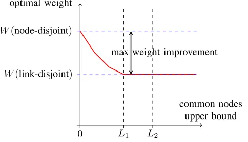
We conclude by describing the space of tractable link-disjoint solutions (depicted in Fig. 6) covered by the solved problems, namely MWLD-Upper-BCN and MWLD-Max-CN. Specifi-cally, the above algorithmic schemes enable the investigation
0 L1 L2
optimal weight
W(node-disjoint)
W(link-disjoint)
max weight improvement
common nodes upper bound
Fig. 6. Spectrum of link-disjoint solutions covered by MWLD-Upper-BCN Algorithm where L1 andL2 are the minimum and maximum, respectively,
number of common nodes in the optimal link disjoint solution.
of feasible link-disjoint solutions between the optimal node-disjoint and the optimal link-node-disjoint with maximum number of common nodes. The weight of the solution is expected to be improved by relaxing the constraint in the number of common nodes till the optimal link-disjoint with maximum number of common nodes (i.e., the solution of MWLD-Max-CN).
V. DIRECTED-ACYCLIC-GRAPH(DAG) TOPOLOGIES
In this section, we consider the three specified problems in Section II, namely MWLD-Upper-BCN, MWLD-Tight-BCN and MWLD-Lower-BCN in the context of DAGs. We present a polynomial-time algorithmic scheme for all problems (includ-ing the MWLD-Tight-BCN and MWLD-Lower-BCN NP-Hard variants).
Consider a DAG G(V, E) (satisfying |V| = N), a source node s ∈ V and a destination node t ∈ V such that there is a path between s and t. The algorithm has two stages. First, it constructs an auxiliary graph G( ˜˜ V ,E)˜ with V˜ = V and links describing possible Node-Disjoint Shortest Pairs of Paths (NDSPoP) in G. This stage is identical to the first stage of the MWLD-Upper-BCN Algorithm (Fig. 4) with the assumption that Gis now a DAG. We refer to the weight of a link (describing the weight of the minimal-weight path pair) between two nodes u, v inG˜ as w(u, v). Then, based on the˜ new graph, the second stage of the algorithm calculates for every destination nodet∈V and a given number of common nodesc∈[0, N−2], a link-disjoint path-pair from stotwith exactlyc common nodes of a minimal weight.
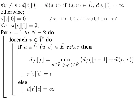
For the second stage, described in Fig. 7, we keep two-dimensional arrays d[N][N],π[N][N]. For a node v ∈V˜ and c∈[0, N−2], after thecth iteration, we would like the value of d[v][c] to describe the weight of a link-disjoint path-pair betweenstovinGhaving exactlyccommon nodes. We keep inπ[v][c]the previous common node of path-pair betweensto v withccommon nodes having a minimal weight.
We start by setting d[v][0] = ˜w(s, v) if a link (s, v) exists in G˜ and d[v][0] = ∞ is such a link does not exist. Then, in iteration c ∈ [1, N−2], for each v ∈ V˜ we set d[v][c] = minu∈V|(u,v)∈E˜ d[u][c−1] + ˜w(u, v)
[image:7.612.312.554.62.201.2]
Input: G( ˜˜ V ,E)˜ - auxiliary graph with NDSPoP links,s - source,t- destination,w˜e- link weight,
Output:
d[N][N]- link-disjoint path weight with given number of common nodes, π[N][N]- link-disjoint paths.
∀v6=s:d[v][0] = ˜w(s, v)if(s, v)∈E,˜ d[v][0] =∞ otherwise;
d[s][0] = 0; /* initialization */ ∀v:π[v][0] =∅;
forc= 1toN−2 do foreach v∈V˜ do
if u∈V˜|(u, v)∈E˜ existsthen
d[v][c] = min
u∈V˜|(u,v)∈E˜ d[u][c−1] + ˜w(u, v)
π[v][c] =u
else
[image:8.612.54.289.137.311.2]d[v][c] =∞
Fig. 7. Algorithm for MWLD-Upper-BCN, MWLD-Tight-BCN and MWLD-Lower-BCN problems in DAGs
such link exists). Likewise, we setπ[v][c]to be the nodeu ob-taining this minimum. The algorithm properties are established by the following theorem.
Theorem 5.1:Consider a DAGG(V, E)with nodess, v∈V. AfterN−2 iterations the valued[v][c]describes the minimum weight of a link-disjoint path-pair betweenstov with exactly ccommon nodes.
Proof: By induction on c. Clearly, with c = 0 common nodes the link-disjoint path-pair is composed of node-disjoint pair of paths that represent a link in G. A path pair with˜ c ≥ 1 common nodes between s and v can be described as a composition of a link-disjoint path pair withc−1 common nodes betweensto some nodeutogether with a node-disjoint pair of path between u to v. Note that in a DAG, unlike a general graph, such composition necessarily results in a link-disjoint path pair betweensandv. The existence of a common link between the two components is impossible as it requires the existence of a cycle. Notice that the maximal number of common nodes cannot be larger thanN−2.
By Theorem 5.1, we can find the solution to each of the problems based on the bound on the number of common nodes. This is done by considering the minimum among the values of d[t][c] for the allowed values of c, i.e. c ∈ [0, k] in the MWLD-Upper-BCN problem,c=kin the MWLD-Tight-BCN problem andc∈[k, N−2]in the MWLD-Lower-BCN problem. The paths can be found by the corresponding values ofπ[t][c], identically to the to the third stage of the MWLD-Upper-BCN Algorithm (Fig. 4).
Time complexity: As stated by Theorem 4.2, we can con-struct the auxiliary graph and calculate its links in O(N+N2·
D(N, M)) =O(N +N2·(M +N·log(N))). In the second stage, we can consider, up toN times, each of theO(N2)links.
The total complexity is thusO(M ·N2+N3·log(N))).
VI. SIMULATIONSTUDY
In this section, we demonstrate the advantages of allowing common nodes on the link-disjoint paths on typical network topologies. Accordingly, we examine the gap in the quality of solution between the optimal node-disjoint paths and the optimal link-disjoint paths by executing the MWLD-Upper-BCN Algorithm described in Section IV. Specifically, for all possible source-destination pairs, we check the percentage of link-disjoint optimal solutions having a certain number of common nodes. Given that a significant number of solutions contain a common node, we evaluate the improvement of allowing common nodes in the quality (in terms of weight) of the optimal solution. Most notably, already by allowing a single common node the maximal weight improvement can be approached, as it improves the total weight of almost alls−t pairs with common nodes in their optimal link-disjoint solution. Thus, the further improvement for largerk values is limited.
A. Setup
We generated random network topologies following the layout of real-world topologies. Each network consists of 40 nodes and either 107,65 or 78links. We divided the network nodes into two sets: Type A nodes are expected to be common in the link-disjoint paths; and Type B nodes are regular network nodes. The links weightwe is generated based on the type of the end-nodes, as follows:
• Type A - Type A: set to 1,
• Type A - Type B: random between 1 and 10,
• Type B - Type B: random between 1 and x.
The links are assumed to be bidirectional having the same weight for both directions. This classification evaluates a scenario of few beneficial (Type A) nodes, such as a data center, at which most of the traffic crosses, while Type B represents a regular node, such as a client. The Type A nodes are connected with high-performance links, while the rest of the network (Type B) nodes linked with low-performance links between themselves and intermediate-performance links to Type A nodes.
0.8 0.9 1
1 2 3 4
relati v e impro v ement
upper boundk x= 10 x= 100 x= 1000
(a) 8 Type A nodes
0.8 0.9 1
1 2 3 4
upper boundk x= 10 x= 100 x= 1000
[image:9.612.322.559.59.208.2](b) 12 Type A nodes
Fig. 8. Relative weight improvement compared to the maximum between the optimal link-disjoint and optimal node-disjoint solution in aN = 40, M = 107network with differentxvalues (representing maximal link weight between two Type B nodes).
0.4 0.5 0.6 0.7 0.8 0.9 1
0 1 2 3 4
optimal
s
−
t
pairs
upper boundk x= 10 x= 100 x= 1000
(a) 8 Type A nodes
0.4 0.5 0.6 0.7 0.8 0.9 1
0 1 2 3 4
upper boundk x= 10 x= 100 x= 1000
(b) 12 Type A nodes
Fig. 9. Percentage of minimal weight MWLD-Upper-BCN solutions compared to alls−tpairs in aN = 40, M = 107network with different xvalues (representing maximal link weight between two Type B nodes).
and optimal node-disjoint solution, i.e. WN−Wk
WN−WL. Then, we
investigate the average relative improvement over all possible source-destination pairs.
B. Results
Fig. 8 shows that in network with 40 nodes allowing even a single common node in the link-disjoint solution more than 80% of the maximal weight improvement can be reached. This is true even if we consider 8 (Fig. 8a) or 12 (Fig. 8b) Type A nodes from the 36 nodes of degree 4 or larger. Although the weight of Type B - Type B links were generated in significantly different ranges (e.g., between 1 and 1000 if x= 1000), the relative improvement is similar for each link weight setting. However, there is a large difference in the number of s−t pairs where the solution weight can be improved with allowing more common nodes, presented in Fig. 9. With 8 Type A nodes in Fig. 9a almost 90% of source target pairs have an optimal node-disjoint solution with x= 10, i.e., when all link weights fall within the range of 1−10. On the other hand, when the weights of Type B - Type B links are selected from a larger range, less than 60% ofs−tpairs have an optimal link-disjoint solution with 0 common nodes. This is because withx= 1000
0.4 0.5 0.6 0.7 0.8 0.9 1
0 1 2 3 4
optimal
s
−
t
pairs
upper boundk 65 links 78 links 107 links
(a) 8 Type A nodes
0.4 0.5 0.6 0.7 0.8 0.9 1
0 1 2 3 4
upper boundk 65 links 78 links 107 links
(b) 12 Type A nodes
Fig. 10. Percentage of minimal weight MWLD-Upper-BCN solutions com-pared to alls−tpairs inN= 40node networks with different link numbers.
0.4 0.5 0.6 0.7 0.8 0.9 1
1 2 3 4
relati v e impro v ement
upper boundk 8 A nodes 12 A nodes 16 A nodes
(a)N= 40, M= 107
0.4 0.5 0.6 0.7 0.8 0.9 1
1 2 3 4
upper boundk 8 A nodes 12 A nodes 16 A nodes
[image:9.612.53.294.60.206.2](b)N= 40, M= 78
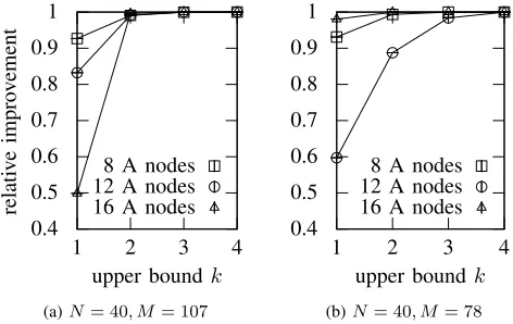
Fig. 11. Relative weight improvement compared to the maximum between the optimal link-disjoint and optimal node-disjoint solution with different number of Type A nodes.
it is beneficial to have a Type A node in common in the link-disjoint solution, as its adjacent links have much lower weight (between 1 and 10) than the other links in the network (between 1 and 1000). This is depicted in Fig. 9a, where for x= 1000 even allowing a third and fourth common node lowers the total weight of about 10% of the connections and allows to solve them to optimality (i.e., their minimum cost link-disjoint path-pair contained 3 and 4 common nodes, respectively). We should also note that the weight improvement introduced by a third and fourth common node is relatively small (in Fig. 8a almost all weight improvement is achieved with 2 common nodes), as their total weight was already improved by allowing one and two common nodes.
In Fig. 9b already about 70% of s−t pairs have a link-disjoint optimal solution with 0 common nodes. This is due to the fact that with 12 Type A nodes almost all of the link weights fall within the range of 1 and 10, as the number of Type B -Type B links is not significantly more than the other links. Thus, there are only a limited number ofs−tpairs which lies within an “island” of Type B nodes. Furthermore, with already two common nodes the maximal weight improvement can be reached except withx= 1000.
[image:9.612.322.558.246.395.2] [image:9.612.55.291.263.410.2]nodes, we selected the x= 1000scenario for further investi-gation, which encourages the appearance of common nodes in the optimal link-disjoint solution. Fig. 10 depicts the percentage of the source-destination pairs for which MWLD-Upper-BCN with an upper bound of k = 0,1,2,3 and4 on the common nodes gives the same (optimal) weight as the link-disjoint path-pair. As expected, by allowing more common nodes in the link-disjoint path-pairs, the number of requests solved to optimality increases. As one can observe, the optimal path-pair is node-disjoint for50%−70%of the source-destination pairs (k= 0). Furthermore, already with an upper bound of k = 4 on the number of common nodes the optimal link-disjoint path pairs were obtained, i.e., none of the link-disjoint paths contained more than 4 common nodes, although in these topologies either 8 or 12 Type A nodes were considered. It is also interesting to note that the improvement of MWLD-Upper-BCN is the largest (54%) in the densest network (M = 107 links) for 8 Type A nodes. However, by increasing the number of Type A nodes from 8 to 12, the maximal weight improvement of MWLD-Upper-BCN decreases to 32%.
Fig. 11 depicts the relative improvement of MWLD-Upper-BCN in a dense (Fig. 11a with average degree of 5.2) and in a sparse (degree 3.9 in Fig. 11b). It is important to note that, although the weight decrease of the MWLD-Upper-BCN solution is low, it is beneficial to 20%−50% of the source-destination pairs even fork= 1in the investigated topologies. Furthermore, the 50% of the gap between the node-disjoint and link-disjoint weight is reached with a single common node, while almost all requests can be solved withk= 2close to op-timality. We conclude that MWLD-Upper-BCN has the largest weight improvement in relatively dense networks (average degree around 5) and with a limited number of Type A nodes (10%-20% of all nodes). We believe that typical real-world network topologies and application scenarios where common nodes are required fall within these categories, respectively.
VII. CONCLUSIONS
We studied the problem of finding a minimum weight link-disjoint pair of paths allowing a certain (bounded) number of common nodes. We formalized three variants of the problem, where the number of common nodes satisfies either an upper-bound, a lower-bound or a tight-bound restriction. We estab-lished the NP-Hardness of the lower-bound and the tight-bound problems, while for the upper-bound problem, we proposed a polynomial-time algorithmic solution. Moreover, we also described a polynomial-time algorithm for the problem that aims to find a minimum weight link-disjoint pair of paths with a maximum number of common nodes. Under the topological restriction of a DAG, we established an efficient algorithmic scheme for all problem variants (namely, the upper-bound, lower-bound and tight-bound problem). Finally, through simu-lations, we analyzed the gap between the optimal node-disjoint and the optimal link-disjoint solutions.
Acknowledgment: This article is based upon work from COST Action CA15127 RECODIS, supported by COST (Eu-ropean Cooperation in Science and Technology). J. Yallouz was
supported by the Israeli Ministry of Science and Technology. O. Rottenstreich was supported by the Rothschild Yad-Hanadiv fellowship. P. Babarczi was supported by the J´anos Bolyai Research Scholarship of the Hungarian Academy of Sciences (MTA) and by the Hungarian Scientific Research Fund (OTKA K108947). The research of A. Orda was supported by Grant No. 2010414 from the United States-Israel Binational Science Foundation (BSF).
REFERENCES
[1] J. W. Suurballe, “Disjoint paths in a network,”Networks, vol. 4, no. 2, pp. 125–145, 1974.
[2] J. W. Suurballe and R. E. Tarjan, “A quick method for finding shortest pairs of disjoint paths,”Networks, vol. 14, no. 2, pp. 325–336, 1984. [3] K. Menger, “Zur allgemeinen kurventheorie,”Fundamenta Mathematicae,
vol. 10, 1927.
[4] P. Elias, A. Feinstein, and C. Shannon, “A note on the maximum flow through a network,”IRE Trans. on Information Theory, vol. 2, no. 4, pp. 117–119, December 1956.
[5] C. Li, S. McCormick, and D. Simchi-Levi, “The complexity of finding two disjoint paths with min-max objective function,” Discrete Applied Mathematics, vol. 26, no. 1, pp. 105–115, 1990.
[6] D. Xu, Y. Chen, Y. Xiong, C. Qiao, and X. He, “On the complexity of and algorithms for finding the shortest path with a disjoint counterpart,”
IEEE/ACM Trans. Netw., vol. 14, no. 1, pp. 147–158, 2006.
[7] A. Orda and A. Sprintson, “Efficient algorithms for computing disjoint QoS paths,” inIEEE INFOCOM, 2004.
[8] L. Guo, K. Liao, H. Shen, and P. Li, “Brief announcement: Efficient approximation algorithms for computing k disjoint restricted shortest paths,” inACM SPAA, 2015.
[9] R. Banner and A. Orda, “The power of tuning: a novel approach for the efficient design of survivable networks,”IEEE/ACM Trans. Netw., vol. 15, no. 4, pp. 737–749, 2007.
[10] J. Yallouz and A. Orda, “Tunable QoS-aware network survivability,” in
IEEE INFOCOM, 2013.
[11] J. Yallouz, O. Rottenstreich, and A. Orda, “Tunable survivable spanning trees,” inACM SIGMETRICS, 2014.
[12] T. Cormen, C. Leiserson, R. Rivest, and C. Stein, Introduction to algorithms. MIT press, 2001.
[13] R. Bhandari, Survivable networks: algorithms for diverse routing. Springer, 1998.
[14] S. Fortune, J. Hopcroft, and J. Wyllie, “The directed subgraph homeo-morphism problem,”Theoretical Computer Science, vol. 10, no. 2, pp. 111 – 121, 1980.
[15] Y. Perl and Y. Shiloach, “Finding two disjoint paths between two pairs of vertices in a graph,”J. ACM, vol. 25, no. 1, pp. 1–9, Jan. 1978. [16] Y. Shiloach, “A polynomial solution to the undirected two paths problem,”
J. ACM, vol. 27, no. 3, pp. 445–456, Jul. 1980.
[17] T. Tholey, “Solving the 2-disjoint paths problem in nearly linear time,” inSTACS, 2004.
[18] M. R. Garey and D. S. Johnson,”Computers and Intractability: A Guide to the Theory of NP-Completeness”. W. H. Freeman & Co., 1979. [19] A. Bj¨orklund, T. Husfeldt, and S. Khanna, “Approximating longest
directed paths and cycles,” inICALP, 2004.
[20] K. Ioannidou and S. D. Nikolopoulos, “The longest path problem is polynomial on cocomparability graphs,”Algorithmica, vol. 65, no. 1, pp. 177–205, 2013.
[21] K. Ioannidou, G. B. Mertzios, and S. D. Nikolopoulos, “The longest path problem has a polynomial solution on interval graphs,” Algorithmica, vol. 61, no. 2, pp. 320–341, 2011.