Chapter
IV
Regression and correlation
analysis
...
Purpose of
Chapter
To measure of the strength of the
relationship between two or more
variables: Correlation Analysis.
Establish
a mathematical model
to
predict or estimate the value of one
variable given a value of another(s)
variable(s): Regression Analysis
Contents
If the value of r is 1.0, there is a perfect direct or positive linear (straight-line) relationship. If the value of r is -1.0 indicates a perfect inverse or negative linear relationship, i.e. “y” increases uniformly as “x” decreases, and 1 indicates a perfect direct linear relationship, i.e. “x” and “y” move uniformly together. A value of close to 0 indicates no correlation. Note that correlation can determine that a relationship exists between variables but says nothing about the cause or directional effect.
This technique is appropriate when: the degree of association between two metric-scaled (interval or ratio) variables is to be examined. • Illustrative research question this technique can answer for example:
Is there a significant relationship between customers' age (measured in actual years) and their perceptions of our company's image (measured on a scale of 1 to 7)?
Simple Regression Analysis is often used to determine the effect of independent variables on a dependent variable. Regression measures the relative impact of each independent variable and is useful in forecasting. This technique is appropriate when:
A mathematical function or equation linking two metric-scaled (interval or ratio) variables is to be constructed, under the assumption that values of one of the two variables is dependent on the values of the other.
• Illustrative research question(s) this technique can answer:
Are sales (measured in RWF) significantly affected by advertising expenditures (measured in RWF)? What proportion of the variation in sales is accounted by the variation in advertising expenditures? How sensitive are sales to changes in advertising expenditures?
4.1 Introduction to regression and correlation simple
The regression and correlation analysis is a statistical methodology that is used to predict facts or events. With respect to regression analysis that is done is to evaluate the contribution of one variables with respect to another, i.e. this analysis evaluate how well one variable (independent) help explain to another (dependent). Correlation analysis measures the strength of the association or relationship between variables without considering which the dependent variable is and which are the independent variable.
In other words: Simple Correlation and Regression are concerned with the investigation of two continuous variables.
We might want to know:
If a relationship exists between those variables; if so, how strong that relationship is? What form that relationship takes? Can we make use of that relationship for predictive purposes?
Correlation describes the strength of the relationship. It is not concerned with 'cause' and 'effect'.
Regression describes the relationship itself in the form of a linear or curved equation which best fits the data.
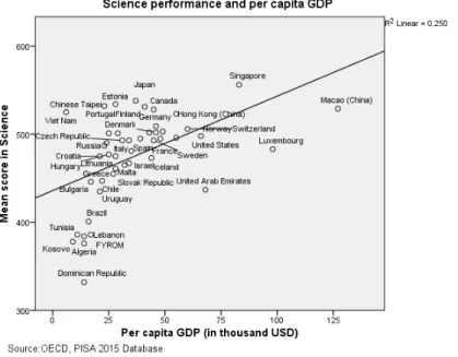
Application: Figure 4.1
The Organization for Economic Co-operation and Development (OECD) released the results of its 2012 global rankings on student performance in mathematics, reading, and science, on the Program for International Student Assessment, or PISA.
The figure shows the simple correlation between the mean scores in mathematics and the expenditure per pupil in secondary education for each of the countries that participated in PISA 2012. It is easy to see that students in countries like Hong Kong and Singapore spend similar amounts of Dollars per Student, achieving very different PISA math scores.
The figure above displays the relationship between national income as measured by per capita GDP and students’ average science performance. The figure also shows a trend line that summarises the relationship between per capita GDP and mean student performance in science. The relationship suggests that 25% of the variation in mean scores is related to per capita GDP. Countries with higher national incomes are thus at a relative advantage, even if the chart provides no indications about the causal nature of this relationship. This should be taken into account particularly when interpreting the performance of countries with comparatively low national income, such as Chinese Taipei and Viet Nam.
Figure 4.3. Relationship between Blood donation and GDP
Methodology
To perform a regression analysis and correlation is advisable to follow the following steps:
1. Collecting data from sources such as questionnaires, forms or databases, texts, brochures, magazines, internet, direct measurements, etc. 2. Draw the scatter diagram, which suggests that model could be used, is a graph showing the intensity and direction of the relationship between two variables. Only up to three-dimensional planes are best seen models suggested, when working with 4 or more variables are graphs surface areas. This question is important: Does the relationship appear to be linear or curved?
3. Calculate the values of the correlation coefficient and the coefficient of determination (note: Correlation coefficient measures the percentage of linear association between variables and coefficients of determination measures the percentage of variability of the dependent variable explained by the independent variable).
5. Estimate the regression line using a processing program with statistical applications (Excel, SPSS, Statgraphics, Minitab, SAS, Statistics, etc.) or by statistical formulas.
6. Make predictions as long as the sample is large enough or when the time is sufficiently reliable predictions are not out of phase with reality. Again to perform a regression analysis and correlation is advisable to follow the following steps:
4.2 Scatter Diagram
Step 1: Scatter Diagram (After collecting the data, draw the scatter diagram)
The starting point is to draw a scatter of points on a graph, with one variable on the X-axis and the other variable on the Y-axis; it is customary represent the dependent variable on the vertical axis and independent on the horizontal axis. When studying the relationship between two variables, one can be considered another cause and a result or effect of the first. Call exogenous or independent variable that causes the effect and endogenous variable. The scatter plots or diagrams give an idea of the relationship (if any) between the variables as suggested by the data. The closer the points are to a straight line, the stronger the linear relationship between two variables.
Scatter diagrams not only show the relationship between variables, but also highlight the individual observations that deviate from the overall relationship. These observations are called outliers or unusual values, which are data points that are separated from the rest.
Example 1
For ten cities, information has been collected on number of civil disturbances (riots, strikes, robberies, criminal damage and violence) over the past year and on unemployment rate. Are these variables associated? The data are presented in the table below.
Table 4.1. Association between Unemployment Rate and Civil Disturbance
City
Unemployment Rate (x)
Civil Disturbances (y)
A 22 25
B 20 21
C 10 6
D 15 8
E 9 1
F 18 22
G 12 7
H 23 25
I 7 3
J 5 0
Scatter diagram
Figure 4.4: Scatter diagram of the Civil Disturbance by Unemployment Rate
Interpretation: There is a direct strong linear association with Civil Disturbance and Unemployment Rate.
Features scatter plots
Depending on how the cloud of points we can obtain the following information: • To determine whether there is a direct or inverse relationship between the variables. • Whether the relationship is strong, moderate or weak.
• Determine if the ratio is set to a linear model or a different mathematical model (e.g. curvilinear model, etc).
X 6 5 4 3 2 1 0 Y 7 6 5 4 3 2 1 X 6 5 4 3 2 1 0 Y 7 6 5 4 3 2 1 X 6 5 4 3 2 1 0 Y 6 5 4 3 2 1 0
Different scatter plots and their respective regression models for them
4.3 Coefficient of Correlation
Step 2: Analysis of Coefficient of Correlation ( ) (Pearson r)
When we study two or more variables simultaneously we are interested in finding a relationship (if it exists) between the two or more variables under study.
The concept of correlation is a statistical tool which studies the relationship between two or more variables and involves various methods and techniques used for studying and measuring the extent of the relationship between them.
“Two variables are said to be in correlation if the change in one of the variables results in a change in the other variable”. For example: The series of sales revenue and advertising expenditure of two companies in a particular year.
A correlation (r> 0) means that there is a Perfect Direct or between the two variables. This means that high scores on X are associated with high values in Y, while low scores on X are associated with low values en Y.
A correlation (r <0) means that there is a Perfect Inverse or negative linear relationship between two variables. This means that low scores on X are associated with high values in Y, while high scores on X are associated with low values en Y.
A correlation (r 0) when is close to zero, is interpreted as the absence of a linear relationship between two variables (no correlation).
Outliers A score of "outlier" is one or more extreme scores in a variable (for example if a variable subjects typically score between 20 and 35 points, the value 80 should be considered "suspect" in principle).
This security severely affects the correlation, especially if we work with small samples. The distortion is typically increase in a "spurious" the degree of linear relationship.
An example of "outlier" can be seen in the chart of alongside
The extreme score (x = 10, y = 10) produces a spurious linear relationship (r = 0.935), since this score if we remove the linear relationship does not exist (r = 0).
Types of Correlation
There are two important types of correlation. They are:
Direct (positive) or Inverse (negative) correlation.
If the values of the two variables deviate in the same direction i.e. if an increase (or decrease) in the values of one variable results, on an
average, in a corresponding increase (or decrease) in the values of the other variable the correlation is said to be direct or positive.
Some examples of series of direct correlation are:
Household income and expenditure;
Heights and weights;
Price and supply of commodities;
Amount of rainfall and yield of crops;
Ice cream sales and temperature (as temperature goes up, ice cream sales go up).
Correlation between two variables is said to be inverse or negative if the variables deviate in opposite direction. That is, if increase in the values of one variable results on an average, in corresponding decrease in the values of other variable.
Some examples of series of inverse correlation are:
TV viewing and class grades-students, who spend more time watching TV tend to have lower grades (or phrased as students with higher grades tend to spend less time watching TV);
Hot chocolate sales and temperature (as temperature goes down, hot chocolate sales go up);
The sales volume of large vehicles is negatively correlated with the price of gasoline;
Quantity demanded for car and price of car.
Linear correlation coefficient (Pearson r)
To quantify the degree of linear relationship between two variables we use the correlation coefficient of Pearson (r). The “r” is given by the following formula:
, also
r = coefficient of correlation n= number of pair of the data ∑x= the summation of the x score ∑y= the summation of the y score
∑xy= the summation of the crossproducts of the scores ∑x2= the summation of the squared scores on x ∑y2= the summation of the squared scores on y
Interpretation “r” Pearson; r is an index of the strength of the linear relationship between two or more variables. While a value of 0.00 indicates no linear relationship and a value 1 indicates a perfect linear relationship. For example when the value is between 0.00 and .+/- 0.20 describes a weak, and when the values are between +/- 0.20 and +/- 0.60 would be moderate, and values greater than +/- 0.60 would be strong. Nevertheless, that these labels are arbitrary guidelines and will not be appropriate or useful in all possible research situation.
For ten cities, information has been collected on number of civil disturbances (riots, strikes, and so forth) over the past year and on unemployment rate. Are these variables associated? The data are presented in the table below. Columns have been added for all necessary sums.
Table 4.2. Association between Unemployment Rate and Civil Disturbance
City
Unemployment Rate (x)
Civil
Disturbances (y) X2 Y2 XY
A 22 25 484 625 550
B 20 21 400 441 420
C 10 6 100 36 60
D 15 8 225 64 120
E 9 1 81 1 9
F 18 22 324 484 396
G 12 7 144 49 84
H 23 25 529 625 575
I 7 3 49 9 21
J 5 0 25 0 0
141 118 2361 2334 2235
The correlation coefficient is:
Interpretation: The correlation between two variables is .964, which indicates a strong direct linear association. Therefore, when the number of unemployment rate increases, the civil disturbance increase at the same time.
Hypotheses of correlation
We will use a two-tailed test for significance at α=.05. The hypotheses are:
Ho: ρ = 0 (there is no association between civil disturbance and unemployment rate) Ha: (There is an association between them)
The decision rule is:
For a two-tailed test using d.f. = n – 2 (degrees of freedom)
Reject Ho if tcalc >tprob. Or if tcalc < tprob Test statistic
Using the SPSS output: If Sig <.05 rejects the null hypothesis, otherwise we cannot reject Ho. The output of SPSS is:
Figure 4.6. Correlations
Unemployment
Rate DisturbancesCivil Unemployment
Rate
Pearson
Correlation 1
.964**
Sig. (2-tailed) .000
N 10 10
Civil Disturbances Pearson
Correlation .964** 1
Sig. (2-tailed) .000
N 10 10
**. Correlation is significant at the 0.01 level (2-tailed).
Make decision and interpret result: We reject the Null Hypothesis given a Sig= .000 < .05, therefore at 5% of level of significance we
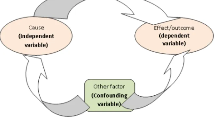
conclude that there is a strong direct association between unemployment rate and civil disturbance ( r = .964**). A Caveat
It must, however, be considered that there may be a third variable related to both of the variables being investigated, which is responsible for the apparent correlation. Correlation does not imply causation. Also, a nonlinear relationship may exist between two variables that would be inadequately described, or possibly even undetected, by the correlation coefficient.
4.4 Coefficient of Determination
Step 3. Coefficient of Determination (Goodness of Fit)
If we wish to know the proportion of variance in “Y” explained by “X”, we can calculate the coefficient of determination. Coefficient of determination or Goodness of fit is measured by:
r2 = (r)2 x 100; and express your interpretation in percentage.
From example 1, the correlation coefficient “r” was: r = .964. Therefore, r2= (.964)2 x100 = 92.9% ≈ 93%
The 'goodness of fit' or coefficient of determination indicates that the 93% of the variance in civil disturbance can be explained by the variance in unemployment rate. What is means in other hands that 93% of the variation in civil disturbance is explained by the unemployment rate.
The output of SPSS is for coefficient of determination (R Square):
Figure 4.7. Model Summaryb
Model R R Square
Adjusted R Square
Std. Error of the
Estimate Durbin-Watson
1 .964a .929 .920 2.886 1.969
a. Predictors: (Constant), Unemployment Rate b. Dependent Variable: Civil Disturbances
Interpretation: r2 = .929, therefore 93% of the variation in civil disturbance is explained by unemployment rate. 4.5 Regression Analysis
Step 4. Regression Equation
Regression is another technique for measuring the linear association between a dependent and independent (or predictor) variable. If two variables are significantly correlated, and if there is some theoretical basis for doing so, it is possible to predict values of one variable from the other.
Regression Analysis, in general sense, means the estimation or prediction of the unknown value of one variable from the known value of the other variable. It is one of the most important statistical tools which are extensively used in almost all Sciences – Natural, Social and Physical. It is specially used in business and economics to study the relationship between two or more variables that are related causally.
Prediction or estimation is one of the major problems in almost all the spheres of human activity. The estimation or prediction of future production, consumption, prices, investments, sales, profits, income etc. are of very great importance to business professionals. Similarly, population estimates and population projections, Revenue and Expenditure etc. are indispensable for economists and efficient planning of an economy.
Models of regression: Linear
Quadratic
Cubic
Logarithmic
Linear function
It is called a linear function of one variable, a function of the form:
: Y intercept (value of “Y” when “X”=0)
: The slope is the change in Y due to a corresponding change of one unit in X.
Power
Compound
Logistics
Exponential Multiple linear
Simple Linear Regression Model
Equation of Simple Linear Regression Model
Suppose we have a sample of size ‘n’ and it has two sets of measures, denoted by ‘x’ and ‘y’. We can predict the values of ‘y’ given the values of ‘x’ by using the equation, called the REGRESSION EQUATION.
Where the coefficients and are given by:
Continue example 1:
We want to show the relationship between civil disturbances and unemployment rate with the first example studied. The data are given in Table 4.1 of this chapter. (See page 4)
Is there a significant linear relationship between two variables? Calculate the regression line of civil disturbance based on unemployment rate. How much increases or decrease the civil disturbance for each 1% of unemployment rate?
Where, e = residual, it is the difference between the actual value of the dependent variable and the estimated value of the dependent variable in the regression equation.
ei =Yi - (the residual)
Yi = actual value of the dependent variable
=estimated value of the dependent variable (“Y hat”)
The β0 is estimated intercept of the Y axis, and is estimated slope of the line (the regression coefficient) The coefficients and are given by:
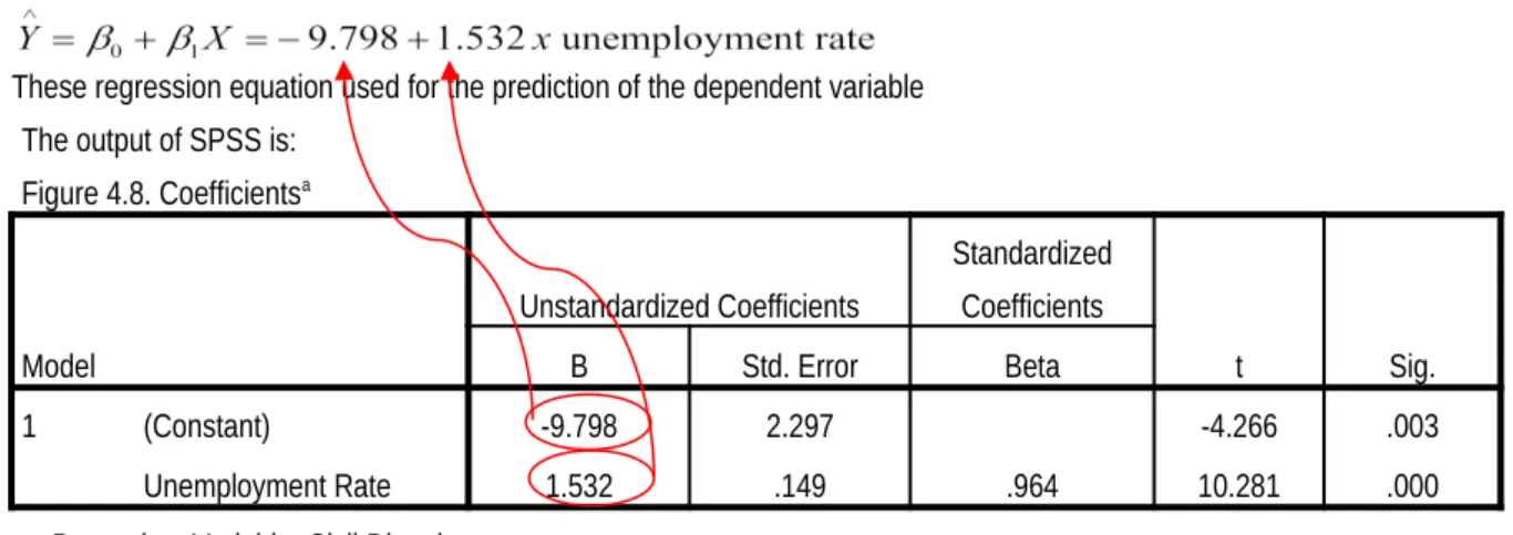
A slope 1.532 means that for every units change in X (for every increase of 1 in the unemployment rate), there was a change of 1.532 units in Y (the number of civil disturbances increased by 1.532).
The least-squares regression equation is
These regression equation used for the prediction of the dependent variable The output of SPSS is:
Figure 4.8. Coefficientsa
Model
Unstandardized Coefficients
Standardized Coefficients
t Sig.
B Std. Error Beta
1 (Constant) -9.798 2.297 -4.266 .003
Unemployment Rate 1.532 .149 .964 10.281 .000
a. Dependent Variable: Civil Disturbances
In terms of hypothesis testing Ho: = 0
Ha:
, here t = 10.281 with a value P_value or Sig = .000 (sig < 0.05)
Make a decision and interpret the result:
Sig.= .000 is less than .05, therefore we reject null hypothesis, and we conclude at level of significance 1% that the dependent variable values depend on the values of the independent variable, i.e. that the Civil Disturbances depends on Unemployment Rate.
Prediction of Civil Disturbance
What number of civil disturbance in these cities would you predict for an unemployment rate of 25?
The best estimate of the civil disturbances is obtained by substituting the value of 25 for that of the independent variable, x, and calculating the corresponding value of the civil disturbances.
Estimated civil disturbances
Interpretation: Thus we expected 29 of number of civil disturbance if unemployment rate is 25.
4.6 Assumptions of the Regression Model (errors)
When you choose to analyze your data using linear regression, part of the process involves checking assumptions that are required for linear regression to give you a valid result data you want to analyze:
1. The variables should be measured at the continuous level (i.e., they are either interval or ratio variables) 2. Linearity: linear relationship between x and y (check in scatter diagram)
3. Normality: the residuals are normally distributed
5. Autocorrelation
Autocorrelation exists when independent variable in a regression equation are highly correlated among themselves. If only two predictors are correlated, we have autocorrelation.
The most common test for autocorrelation is the Durbin-Watson statistic is a test to find out the serial correlation between adjacent error terms. The range of this statistic ranges from 0 to 4.
DW < 2 suggest positive autocorrelated (common) DW ≈ 2 suggest no autocorrelated (ideal) DW > 2 suggest negative autocorrelated (rare)
A rule of thumb is that test statistic values in the range of 1.5 to 2.5 are relatively normal. Any value outside this range could be a cause for concern.
Figure 4.9. Checking the residuals are nonautocorrelated (Colinearity) Model Summaryb
Model R R Square Adjusted RSquare
Std. Error of the
Estimate Watson
Durbin-1 .964a 0.929 0.92 2.886 1.969
a. Predictors: (Constant), Unemployment Rate (x) b. Dependent Variable: Civil Disturbances (y)
In the example, Durbin-Watson = 1.969. It is a value around 2, indicating that the residuals are nonautocorrelated; and therefore we can assume that the collinearity is not observed.
Normal distribution of residuals
A residual is the difference between the observed and model-predicted values of the dependent variable. The residual for a given product is the observed value of the error term for that product.
A histogram or P-P plot of the residuals will help you to check the assumption of normality of the Residuals
Figure 5.9. Checking the Normality of the Residuals
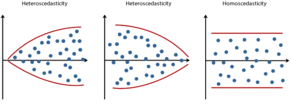
Figure 4.10. Checking Homoscedasticity of Residuals
Example 2
We shall consider whether there is any relationship between the Sales and Advertising Expenditure of a small local bakery.
Table 4.3. Association between Advertising and Sales in RWF
Year Advertising(Rwf'000) (Rwf'000)Sales
1990 3 40
1991 3 60
1992 5 100
1993 4 80
1994 6 90
1995 7 110
1996 7 120
1997 8 130
1998 6 100
1999 7 120
2000 10 150
Step 1. Plot a scatter diagram of the data.
We are looking for a linear relationship with the bivariate points plotted being reasonably close to the, yet unknown, 'line of best fit'. At this stage no 'causality' is implied but it makes sense to use the same diagram for the addition of the regression line later, so the potentially dependent variable should be identified and plotted on the vertical axis.
Figure 4.11 Scatter Diagram for Advertising and Sales in RWF
Interpretation: Seems to indicate a straight line relationship, due to that all points fairly close to a 'line of best fit'. The strength of the relationship will therefore be quantified by calculating the correlation coefficient and testing it for significance.
Step 2. Calculate the correlation coefficient.
Interpretation: r= .958, Is the size of this correlation coefficient, .958, large enough to claim that there is a direct strong relationship between advertising and sales. The test statistic obtained above in this case seems very close to 1, but is it closes enough?
Interpret the following Outcomes of SPSS software.
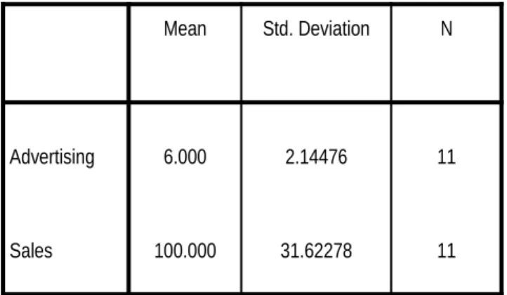
Figure 4.12. Descriptive Statistics
Mean Std. Deviation N
Advertising 6.000 2.14476 11
Sales 100.000 31.62278 11
Figure 4.13. Coefficient of Correlation
Advertising Sales
Advertising
Pearson Correlation 1 .958**
Sig. (2-tailed) .000
N 11 11
Sales
Pearson Correlation .958** 1
Sig. (2-tailed) .000
N 11 11
**. Correlation is significant at the 0.01 level (2-tailed).
Hypothesis test of correlation
Ho: (there is no association between advertising and sales) Ha: (There is an association between them)
Making a decision and interpret the result:
We reject the Null Hypothesis given a significance of Sig. = .000, therefore at 1% we conclude that there is a strong direct association between advertising and sales.
Test it for significance at the 5% level
(Consider that the coefficient is simultaneously equal to zero) (Coefficient is not equal to zero)
Figure 4.14. ANOVAa
Model Sum of Squares df Mean Square F Sig.
1
Regression 9184.783 1 9184.783 101.400 .000b
Residual 815.217 9 90.580
a. Dependent Variable: Sales b. Predictors: (Constant), Advertising
Decision and interpret result: The significance value of the F statistic is less than 0.05, which means that the variation explained by the model is not due to chance. In other words the p_value or sig. associated with this F value is very small (.000). These values are used to answer the question “Do the independent variables reliably predict the dependent variable?, the answer is, YES!
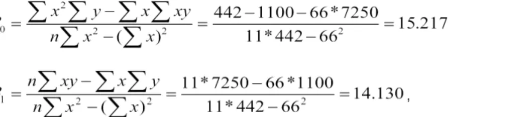
If significant, find the equation of the regression line. Linear regression equation:
The Y intercept β0 is:
,
A slope 14.130 means that for every units change in X (for every increase of 1 in advertising), there was a change of 14.130 units in Y (the sales increased by 14.130).
The least-squares regression equation is:
Outcome of SPSS
Figure 4.15. Coefficientsa
Model Unstandardized Coefficients Standardized Coefficients t Sig.
B Std. Error Beta
1 (Constant) 15.217 8.895 1.711 .121
Advertising 14.130 1.403 .958 10.070 .000
a. Dependent Variable: Sales
What practical use could be made of this equation?
The regression model is used to predict the dependent variable, in this case the sales.
Goodness of Fit or coefficient of determination
How well does this line fit the data? Goodness of fit is measured by (r2 x 100)%.
What percentage of the variation in sales is explained by your model? Figure 4.16. Model Summary
Model r r Square Adjusted r Square Std. Error of the Estimate
1 .958a .918 .909 .64550
a. Predictors: (Constant), Sales
Interpretation: the correlation coefficient r was 0.958 so we have r2=0.9582 x 100 = 91.8% fit. This high value indicates that any predictions made about “y” from a value of “x” will be good.
The 'goodness of fit' indicates the percentage of the variation in the sales which is accounted for by the variation of the advertising. Meaning in other hands that 92% of the variation in sales is explained by the variation in advertising.
Prediction of Sales
Suppose that advertising expenditure for the following month is 12 (Rwf’000), what would he expect his Sales to be?
The best estimate of the Sales is obtained by substituting the value of 12 for that of the independent variable, x, and calculating the corresponding value of the Sales,
Estimated Sales = 15.217 + 14.130 * advertising Estimated Sales =15.217 + 14.130*12
Interpretation: Expected sales would be Rwf 185000 thousand Rwf if advertising expenditure was 12 thousands Rwf
Assignment 4
Short answers
1. The slope (B1) represents:
a. Predict value of y when x=0 b. Predict value of Y
c. Change in Y per unit change in X
2. The Y intercept (B0) represents the:
a. Change in Y per unit change in X b. Predict value of y when x=0 c. Variation around the regression line 3. The coefficient of determination (r2) tells you:
a. The proportion of total variation that is explained b. Whether the slope has any significance
c. Whether the regression sum of squares is greater than the total sum of squares
4. In performing a regression analysis involving two numerical variables, you assume: a. The variance of X and Y are equal
b. That X and Y are independent c. All of the above
5. The residuals represent:
a. The difference between the actual Y values and the mean of Y b. The square root of the slope
c. The difference between the actual Y values and the predicted Y values
6. If the coefficient of correlation (r) = -1.00, then:
a. All the data points must fall exactly on a straight line with a inverse or negative slope. b. All the data points must fall exactly on a straight line with a positive slope
c. All the data points must fall exactly on a horizontal straight line with a zero slope.
7. Assuming a straight line (linear) relationship between X and Y, if the coefficient of correlation (r) = -0.30: a. There is no correlation
b. Variable X is larger than variable Y c. The slope is negative
8. In a simple linear regression model, the coefficient of correlation and the slope: a. May have opposite signs
b. Must have the same sign c. Are equal
11. Haverty’s Forniture is a family business that has been selling to retail customers in the Chicago area for many years. The company advertises extensively on radio, TV, and the internet, emphasizing low prices and easy credit terms. The owner would like to review the relationship between sales and the amount spent on advertising. Below is information on sales and advertising expense for the last four months.
Month Advertising Expense($ millions) RevenueSales
July 2 7
August 1 3
September 3 8
October 4 10
Note: in real life never use a small sample, here there is only one mathematical example for easy to calculate
a. The owner wants to forecast sales on the basis of advertising expense. Which variable is the dependent variable? Which variable is the independent variable?
b. Draw and interpret a scatter diagram
c. Compute and interpret the coefficient of correlation
d. Compute and interpret the coefficient of determination within the context of this problem e. Compute the regression equation
f. Estimate sales for the month of November if invested in advertising 4.5 millions $
Answer: r =.965*, Sig. = .035, r2 =93.1%, ,
12. A Company has just brought out an annual report in which the capital investment and profits were given for the past few years. Find the type of correlation (if it exists).
Capital Investment
“x”(million) Profits “y” (thousands)
16 14
18 13
24 18
36 26
48 38
50 47
22 17
a. Draw and interpret a scatter gram and a freehand regression line. b. Compute and interpret the coefficient of correlation
c. Compute and interpret the coefficient of determination within the context of this problem d. Compute the regression equation
e. Compute a 95% prediction of profits whose capital investment is 60 millions
Answer: r = .969, r2 = 93.9%, ,
13. Why does voter turnout vary from election to election? For municipal election in the six different cities, information has been gathered on the percent of registered voters who actually voted, unemployment rate, average years of education for the city, and the percentage of all political ads that used “negative campaigning” (personal attacks, negative portrayals of the opponent’s record, etc.).
For each relationship:
a. Draw and interpret a scatter dot and a regression line. b. Compute and interpret the coefficient of correlation c. Compute and interpret the coefficient of determination d. Compute the regression equation
e. Predict the voter turnout for a city in which the unemployment rate was 12, a city in which the average years of schooling was 11, and an election in which 90% of the advertising were negative.
f. Assume these cities are a random sample and conduct a test of significance for each relationship.
g. Describe the strength and the direction of the relationships in a sentence. Which (if any) relationships were significant? Which factor had the strongest effect on turnout?
TURNOUT AND EMPLOYMENT Answer: r = .950, r2 =90.3%,
City Turnout Unemployment rate ,
A 55 5
B 60 8
C 65 9
D 72 12
E 68 9
F 70 10
TURNOUT AND LEVEL OF EDUCATION
City Turnout Average years ofschool Answer: r = .941, r2 =88.6%,
A 55 11.9 ,
B 60 12.1
C 65 12.7
D 72 12.8
E 68 12.9
F 70 13.0
TURNOUT AND NEGATIVE CAMPAIGNING
City Turnout Advertisements% of Negative Answer: r =-.694, r2 =48.2%,
A 55 60 ,
C 65 55
D 72 53
E 68 60
F 70 48
Solution: Q13.e.
Coefficientsa
Model
Unstandardized Coefficients
Standardize d Coefficients
t Sig.
B
Std.
Error Beta
1 (Constant) -35.421 27.887 -1.270 .332
Average years of school 6.981 2.044 .492 3.415 .076
Unemployment 1.517 .360 .545 4.213 .052
% of Negative Advertisements -.013 .125 -.011 -.101 .929
a. Dependent Variable: Turnout_Q13
y= 58.44685416