Estimating the Heterogeneity Effects in a Panel Data Regression Model

(1)

E

S

T

I

M

A

T

I

N

G

T

H

E

H

E

T

E

R

O

G

E

N

E

I

T

Y

E

F

E

C

T

S

I

N

A

P

A

N

E

L

D

A

T

A

R

E

G

R

E

S

I

O

N

M

O

D

E

L

1

Nureni Olawale Adeboye,

2

Dawud Adebayo Agunbiade

1

Department of Mathematics & Statistics, Federal Polytechnic, Ilaro, Nigeria. P.M.B 50

2

Department of Mathematical Sciences, Olabisi Onabanjo University, Ago-Iwoye, Nigeria

Corresponding author: Nureni Olawale Adeboye, [email protected]

ABSTRACT: Violation of homoscedasticity assumption in a Panel Data Regression Model (PDRM) implies unequal variability of error terms, and this creates heterogeneity problem in estimation. This research thus attempts to investigate the presence and effect of heteroscedasticity in panel data through the estimation of a specified audit fees PDRM using Pooled ordinary least square (POLS, Least square dummy variable (LSDV) technique where all coefficients vary across individual and Random Effect estimator (REM). A conditional Lagrange multiplier test was developed via a two-way error components model, to examine the presence of heteroscedasticity in the fitted POLS model while Hausman test was used to ascertain the suitability of the LSDV Model over Random effect model and vice-versa. The conditional LM test gave a value of 7.1462 with P-value of 0.000000000000446 which shows that there is presence of unequal variance of MA(1) errors among the residuals of the fitted Pooled OLS model, thereby rendered the estimator inconsistent. Both LSDV and RE models were fitted to take care of the challenges posed by the presence of heteroscedasticity and both models captured the goodness of fit better when compared to the Pooled OLS model. However, the Hausman test revealed that random effect model will not be preferable since p-value of the former is less than 0.05.

KEYWORDS: Heterogeneity, Heteroscedasticity, Conditional Lagrange Multiplier, Panel Data, Audit Fees Model, Panel Data Regression Model.

1.INTRODUCTION

A panel is a cross-section or a kind of data in which observations are obtained on the same set of entities at several periods of time [Fre95, GP09, Hsi03, Ken08, Gre03]. Panel data models examine individual-specific effect, time effect or both in order to deal with heterogeneity/serial correlation of individual effects that may or may not be observed.In this paper, our focus shall only reflect on the problems which affect the cross sectional aspect of panel data, which is the problem imposed by heteroscedasticity. This shall be looked into via a panel data regression model of audit fees.

Heteroscedasticity is one of the associated problems with the Pooled Ordinary Least Squares (POLS)

[GP09]. By heteroscedasticity, we meant the existence of some non- constant variance function in a Panel data regression model (PDRM). [LE00] and [BFN83] confirmed that in the presence of heteroscedasticity, Ordinary least square (OLS) estimates are unbiased, but the usual tests of significance are generally inappropriate and their use can lead to incorrect inferences. Among other things, they suggest that data analysts should correct for heteroscedasticity using Heteroscedasticity Consistent Covariance Matrix (HCCM) whenever there is reason to suspect its presence. The pioneering work of [8] has given rise to further researches on the estimation of heteroscedasticity effects in panel data. Prominent among these works are those of [RWH81, Mag82, HR94, Bal88, BG88, Ran88, Wan89, LS94, Lej06, HG00, Roy02, Phi03, BBP06]. However, these works were concerned with regression models that have to do with one-way error component model while this work is based on two-way error components model. For instance, both [BGT90] and [BG88] were concerned with the estimation of a model allowing for heteroscedasticity on the individual-specific error term i.e., assuming that



_i~ (0, ) while vit ~ IID(0, σ2v). In contrast, [RWH81], [Mag82], [Bal88] and [Wan89] adopted a symmetrically opposite specification allowing for heteroscedasticity on the remainder error term, i.e., assuming that μi ~ IID (0, σ2

μ) while vit~(0, σ 2

(2)

to estimation, [LS94] proposed an adaptive estimation procedure for a one-way error component model allowing for heteroscedasticity of unknown form on the remainder error term, i.e., assuming that μi ~ IID (0, σ2μ) while vit ~ N (0, ), where σ

2

vit is a nonparametric function f( z′it) of a vector of exogenous variables. They also suggest a robust version of [BP80] Lagrange Multiplier (LM) test for no random individual effects, by allowing for adaptive heteroscedasticity of unknown form on the remainder error term. [Lej06] on the other hand, used Maximum Likelihood (ML) Estimation and LM to test for general heteroscedasticity in a one-way error components model while [HG00] proposed a Rao score test for homoscedasticity assuming the existence of individual effects. [Phi03] follows [MT78] in considering a one-way stratified error component model. As unobserved heterogeneity occurs through individual-specific variances changing across strata, [Phi03] provides an algorithm for estimating this model and suggests a bootstrap test for identifying the number of strata. [BBP06] derived an LM test for the null hypothesis of homoscedasticity of the individual random effects assuming homoscedasticity of the remainder error term. In relation to the general heteroscedastic model of [Ran88, Lej06], [BBP06] also derived a joint test for homoscedasticity. Under the null hypothesis, the model is a homoscedastic one-way error component regression model and is estimated by restricted MLE. This is different from [Lej06], where under the null hypothesis, σ2μ = 0, so that the restricted MLE is OLS and not MLE on a one-way homoscedastic error component model. The validity of this model under the null hypothesis is exactly that of [HG00] but it is more general under the alternative hypothesis since it does not assume a homoscedastic remainder error term. This research therefore, intends to examine this opinion on a PDRM tagged Audit Fees Model by deriving a conditional LM test for the presence of heteroscedasticity via a two-way error components model, where zero serial correlation is assumed. Audit fees represent fees a company pays an external auditor in exchange for performing an audit. Prominent among authors who have worked on modelling of audit fees are [AA12a, AA12b, A+13, Gam12, SO13, Has15], but they all conjectured differently from the background knowledge of the audit fees model specified in this research, which is in line with [***90].

2. MATERIAL AND METHODS

2.1. Specification of Audit Fees Model

This model employed the use of four (4) Pre-determined variables namely Profit before Tax (PBT), Total Assets

(TA), Total Liability (TL) and Shareholders Fund (SHF) which shall be originated from panel data of published annual reports of sixteen (16) Nigerian Commercial Banks for periods of ten (10) years. The model as implied by the scope of auditor’s work in CAMA ([***90]) is thus presented as:

(1)

When the model is expressed in an explicit format, we have

(2)

β1, β2, β3, β4 and β5 are parameters to be estimated and εit is a composite error term. Within the context of this research,

In the course of this study, we hope to demonstrate that the conditional variance of increases as each of increases.

Within the context of PDRM, both the parameters and error terms of equation (2) shall be varied based on space that will result into the following equations:

(3)

In estimation, we employ the dummy variable technique (i.e. the differential intercept dummies) to account for the individual effect. Thus the model becomes

= + +

(4)

Where α1 represents the intercept of the first

individual (i.e. bank) and α2, α3, ..., α16 are the

differential intercept coefficients which tell us by how much the intercept of the remaining banks differ from the intercept of the first while which

was not created for the first individual to avoid falling into dummy variables trap. In a situation where all the coefficients are allowed to vary across individuals, we extend equation (4) with the introduction of individual dummies in additive manner. Thus we have

= + +

+

(3)

are the differential slope

coefficients, just as are the differential

intercepts.

Similarly, for the REM, we recalled equation (4) and instead of treating as fixed, we assume that it is a random variable with a mean value of β1. Thus, the intercept value for the individual bank can be expressed as

+ (6)

The individual differences in the intercept values of each bank are reflected in the error term if we substitute equation (7) in (4), we have

(7)

Equation (8) implies

+ (8)

where + εit (9)

Thus, the composite error term consists of two

components (cross section error component) and εit which is the combined time series and cross-section error component.

2.2.Model Estimation Techniques

Here, we provide brief theoretical overview of the three (3) techniques considered in this study.

(i) Pooled OLS: This technique pool the data over i and t into one nT observations, and estimates of the parameters are obtained by OLS using the model

y = X'β + (10)

where y is an nT × 1 column vector of response variables, Xis an nT × k matrix of regressors, β is a (k+1) × 1 column vector of regression coefficients, is an nT × 1 column vector of the combined error terms (i.e ). The Pooled estimator is given

as

(11)

(ii) Fixed Effect Least Square Dummy Variable: Let and be the observations for the unit, be a column of ones, and let be associated vector of disturbances. Then

(12)

Connecting these terms in matrix form gives

(13)

where is a dummy variable indicating the unit.

Let the matrix

then, assembling all NT rows gives;

α (14)

Estimating the equation using OLS gives an estimator

(15)

MD = _,

.

The OLS referred in equation (15) shall be a Within-Group (WG) estimator. According to [Woo12], the within transformation implements the LSDV model better because the regression on de-meaned data yields the same results as estimating the model from the original data and a set of (N-1) indicator variables for all but one of the panel units. It is often not workable to estimate that LSDV model directly because we may have hundreds or thousands of individual panel units in our dataset.

(iii) Random Effect Estimator: Consider a random effect model

(16)

we employ GLS estimator by transforming model (16) into

(17)

We then multiply equation (17) by and takes its difference from equation (16) to have

(18)

Thus, the GLS estimator for the slope parameter of (18) becomes

(19)

(4)

And (the key transformation parameter) is given as

=

(21)

Thus, equation (19) is the specific GLS estimator called Random effect estimator.

2.3.Model Testing

Here, we shall employ a two-way error component model as earlier emphasized, to test for the violation of homoscedasticity assumption in our researched model.

Considering a two-way error component model stated as:

(22)

Within the context of two-way error component, the regression disturbances term can be described by

the equation

(23)

With representing individual-specific effect, representing time-specific effect and the

idiosyncratic remainder disturbance term, which is usually assumed to be well-behaved and independent from both the regressors and . The

two-way error component model can be written in matrix form as

(24)

The disturbance term in equation (24) can be written in vector form as

(25)

Where is an identity matrix of dimension ,

is an identity matrix of dimension , is an identity

matrix of dimension is a vector of ones of

dimension , is a vector of ones of dimension , is a vector of ones of dimension , , is the AR(1) covariance matrix of dimension denotes the kronecker product and

(26) According to [BP80], the function is an arbitrary strictly positive twice continuously differentiable function, vector of unrestricted parameters and is a vector of strictly exogenous regressors which determine the

heteroscedasticity of the individual specific effects and the first element of is one, and without loss of generality, .

Following [BJS10], the variance-covariance matrix of can be written as

(27)

Where is a matrix of ones of dimension dimension and can be expressed as

(28)

is a symmetric matrix of order

2.3.1.Conditional LM Test for ,

In this section, we derive a conditional LM test for presence of individual heteroscedasticity in the absence of serial correlation.

Under normality of the disturbances, the log-likelihood function, of a Lagrange multiplier follows that of a multivariate normal distribution. Thus,

(29)

Where and . In this case, we set , . Thus, becomes , . In order to obtain the conditional LM statistic, we need to obtain the score statistic

and the

Information matrix

. Following

[32], we obtain and as

₍₃₀₎

(31)

Under the variance covariance matrix of the

disturbances as given by equation (27) becomes

(5)

And according to [WK82], the spectral decomposition and inverse of respectively becomes

(33)

Where (34)

Therefore,

2 2 +12 2 4 +1 2 + 2 4

=1 =1 2 2+ 22 1 4 +1 4 + 1 4

Since there’s no serial correlation of which its variance has been expressed as

1 4 (35)

Equation (35) is the solution obtained after maximization of the first order condition, where is the generalized least square

residuals under is the ML estimator of is the evaluated value of . All the components of the score test statistic

evaluated at maximization of the first order condition are all equal to zero except

[K+14].Thus, the partial derivatives under are expressed in vector form as

(36)

Also, we obtain information matrix under the null hypothesis as follow:

(6)

Thus, information matrix under the null hypothesis can be obtained as a symmetric matrix of the form

(37)

(7)

Thus, a conditional statistic under the specified is given as

(39)

Setting

LM statistic also becomes

(40)

Thus, the statistic becomes

(41)

Where

Under statistic is asymptotically distributed as

3.RESULTS AND DISCUSSION

The results of the three models fitted from the analytical techniques discussed and that of the test carried out to showcase the heterogeneity effects, as occasioned by the presence of heteroscedasticity are presented and discussed in this section.

Table 1: Presentation of Pooled OLS Results

Variables Coefficients Standard Error t-value Pr(>|t|)

Intercept 120,970 10,011 12.0840 0.0000

PBT 0.00080588 0.00027278 2.9543 0.0036

TA -0.000026096 0.000012963 -2.0131 0.0458

TL 0.0000080482 0.000035418 2.2724 0.0244

SHF 0.00025419 0.00012246 2.0757 0.0396

Table 2: Conditional Lagrange Multiplier Test for Heteroscedasticity

Z P-value

7.1462 0.000000000000446

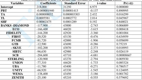
Table 3: Presentation of LSDVM Results that Accounts for Only Individual Effects

Variables Coefficients Standard Error t-value Pr(>|t|)

Intercept 218,000 31250 6.975 0.000000

PBT -0.000001940 0.00001413 -0.137 0.890995

TA 0.000008032 0.000003303 2.432 0.016299

TL 0.0005581 0.0002772 2.014 0.045967

SHF 0.00002475 0.0001289 0.192 0.848021

BANKS -DIAMOND -117,900 43000 -2.743 0.006889

ECO -166,400 46020 -3.615 0.000418

FIDELITY -144,200 42920 -3.360 0.001004

FIRST -20,520 43130 -0.476 0.634959

FCMB -81,720 42880 -1.906 0.058699

GTB -12,500 43690 -0.286 0.75219

- SKYE -102,200 43070 -2.373 0.018993

SIBTC -96,630 42980 -2.248 0.026119

SCB -204,600 43710 -4.681 0.00000667

STERLING -120,900 43270 -2.794 0.005930

UNION -77,310 44620 -1.733 0.085324

UBA -11,780 43400 -0.271 0.786517

UNITY -66,920 43330 -1.545 0.124695

WEMA -138,400 43450 -3.186 0.001782

(8)

Table 4: Presentation of Random Effect Model Results that Accounts for Both Individual and Time Effects (Twoways effects Model)

Effects

Variance

Standard Dev

Shares

Theta (Lambda)

idiosyncratic

5809000000

76210

0.746 -

individual

1894000000

43520

0.243 0.5155

time

85800000

9263

0.011 0.1006

Total

-

0.08774

Variables

Coefficients

Standard Error

t-value

Pr(>|t|)

Intercept

130400

1.6386

0.0000

PBT

0.00061736

26438

2.3351

0.02082

TA

-0.000011315

0.000013033

0.8682

0.38664

TL

0.0000079030

0.000003179

2.4860

0.01398

SHF

0.000099058

0.00012030

0.8234

0.41152

Table 5: Presentation Hausman Test Results

Chi square

Df

p-value

1193.6

4 0.0000

The specified models for POLS, LSDVM and REM from tables 1-3 respectively are given as follows:

(41)

(42)

(43)

The three specified models are statistically significant based on their P-values which are less than 0.05 while there coefficient of determination, indicates that our exogenous variables explained 20.43%, 45.85% and 15.61% variation in the audit fees of Nigerian banks for the years under review respectively for POLS, LSDVM and REM. Meanwhile, the standard errors of regression coefficients for the POLS model are a bit higher than

that of LSDV and REM models. The POLS’s standard errors were due to the inefficiency of POLS estimator as induced by the presence of heteroscedasticity which has not been taken care prior to the model’s fitting. The fact that heteroscedasticity is present in the POLS estimator was established through the conduct of conditional LM test. The LM result is asymptotically chi squared distributed with Z-value of 7.1462 and a P-value of 0.000000000000446, which is far less than the critical value of 0.05. This result prompts the rejection of our null hypothesis and thereby validates the presence of heteroscedasticity in the POLS residual.

The LSDVM seems to be a better model to explain the specified audit fees model as a result of its lower standard errors and higher coefficient of determination, and this is further confirmed by its preference based on Hausman test. Thus, model presented as equation (42) shall be our chosen model for the scientific fitting of audit fees across commercial banks in Nigeria and diaspora. This model, which is non heteroscedastic, presents a superior goodness of fit.

CONCLUSION

Various results obtained in this work generally showed that the behaviours of the three estimators investigated for modeling audit fees vary due to violation of homoscedasticity assumption. The effect heteroscedasticity has on modeling panel data using these techniques for estimating audit fees model with violation of homoscedasticity assumption has been addressed.

(9)

parameters of panel data models, errors have to be independent and homoscedastic. These conditions are so atypical and mostly unrealistic in many real life situations that would have warranted the use of POLS for modeling panel data efficiently, hence the needs for developing a suitable LM test to ameliorate its ugly incidence.

REFERENCES

[AA12a] D. A. Agunbiade, N. O. Adeboye - Estimation of Heteroscedasticity Effects in a Classical Linear Regression Model of a Cross Sectional Financial Data, Journal of Progress in Applied Mathematics, 4 (2012), pp. 18-28.

[AA12b] D. A. Agunbiade, N. O. Adeboye - Estimation under Heteroscedasticity: A Comparative Approach Using Cross Sectional Data. Journal of Mathematical Theory and Modelling, 2 (2012), pp. 1-8.

[A+13] Y. A. Akinpelu, S. O. Omojola, T. O. Ogunseye, O. T. Bada - The Pricing of Audit Services in Nigeria Commercial Banks, Research Journal of Finance and Accounting, 4 (2013), pp. 1-8.

[Bal88] B. H. Baltagi - An alternative heteroscedastic error component model. EconometricTheory, 4(1988), 349-350.

[BG88] B. H. Baltagi, J. M. Griffin - A generalized Error Component Model with Heteroscedastic Disturbances. International Economic Review 29(1988), 745-753.

[BP80] T. S. Breusch, A. R. Pagan - The Lagrange Multiplier Test and its Applications to Model Specification in Economics. Review of Economic Studies (1980), pp. 239-253.

[BBP06] B. H. Baltagi, G. Bresson, A. Pirotte - Joint LM Test for Homoscedasticity in a One-way Error Component Model. Journal of Econometrics, 134(2006), 401-417.

[BFN83] A. L. Bhargava, L. Franzini, W. Narendranathan - Serial correlation and the fixed effects Model, Review of

Economic Studies 49(1983), pp. 533-549.

[BJS10] B. H. Baltagi, B. C. Jung, S. H. Song - Testing for Heteroskedasticity and Serial Correlation in a Random Effects Panel Data Model. Journal of Econometrics, 154 (2010), pp. 122-124.

[BGT90] S. P. Burke, L. G. Godfrey, A. R. Termayne - Testing AR(1) Against MA(1) Disturbances in the Linear Regression Model: An Alternative Procedure, Review of Economic Studies 57 (1990), pp. 135-145.

[Fre95] E. W. Frees - Omitted Variables in Panel Data Models. Canadian Journal of Statistics, 29(1995), pp. 1-23, 1995.

[Gam12] W. El-Gammal - Determinants of Audit fees: Evidence from Lebanon international Business Research, Canadian Center of Science and Education, 5 (2012), pp. 136-145.

[Gre03] H. W. Green (ed.) - Econometric Analysis, Prentice Hall, Upper Saddle River, New Jersey, 2003.

[GP09] D. N. Gujarati, D. C Porter (ed.) - Basic Econometrics. Mc Graw-Hill, New York, 2009.

[Has15] Y. K. Hassan - Determinant of Audit Fees: Evidence from Jordan. Accounting and Finance Research, 4(2015), pp. 42-53, 2015.

[Hsi03] C. Hsiao (ed.) - Analysis of cross-sectional Data, Cambridge University Press Cambridge, 2003.

[HG00] A. Holy, L. Gardiol (ed.) - A Score Test for Individual heteroscedasticity in a One Way Error Components Model in Krishnakumar, J., Ronchelli, Editors, Panel Data Econometrics: Future Directions. Elsevier Amsterdam. Chapter 10 (2000).

(10)

[Ken08] P. Kennedy (ed.) - A guide to Econometrics, Malden, MA: Blackwell Published, 2008.

[K+14] E. Kouassi, M. Mougoue, J. Sango, J. M. Bosson Brou, M. O. Claude, A. A Salisu - Testing for Heteroscedasticity and Spatial Correlation in a Two-way Random Effects Model, Computational Statistics and Data Analysis, 70(2014), pp. 153-171.

[Lej06] B. Lejeune - Full Heteroscedasticity One-way Error Component Model: Pseudo Maximum Likelihood Estimation and Specification Testing, Theoretical Contributions and Empirical Applications. Elsivier Science, Amsterdam, pp. 31-66, chapter 2 (2006).

[LE00] J. S. Long, L. H. Ervin - Using

Heteroscedasticity Consistent Standard

Errors in the Linear Regression

Model. The American Statistician, 54, (3), 217-224, 2000.

[LS94] Q. Li, T. Stegnos - An Adaptive Estimation in the Panel Data Error

Component Model with

Heteroscedasticity of unknown form, International Economic Review 35(1994), pp.981-1000.

[Mag82] J. R. Magnus - Multivariate Error Components Analysis of Linear and Non Linear Regression Models by Maximum Likelihood, Journal of Economerics, 19(1982), pp. 239-285.

[MT78] P. Mazodier, A. Trognon - Heteroskedasticity and stratification in error Components models, Annales de L’INSEE 30-31(1978), pp. 451-482.

[Phi03] R. L. Phillips - Estimation of a Stratified Error Components Model. International Economic Review, 44(2003), pp. 501-521.

[Ran88] W. C. Randolph - A transformation for Heteroscedastic Error Components Regression Models, Economic Letters. 1988.

[Roy02] N. Roy - Is Adaptive Estimation Useful for Panel Models with Heteroscedasticity in the Individual Specific Error Component? Some Monte Carlo Evidence. Econometric Review, 21, pp. 189-203, 2002.

[RWH81] C. R. Rao, R. A. Wayne, I. K. Hogdson - The Theory of Least Squares when the Parameters are Stochastic and its Application to the Analysis of Growth Curves Biometrika, 52(1981), pp. 447-58.

[SO13] K. A. Soyemi, J. K. Olowookere - Determinants of External Audit Fees: Evidence from the Banking Sector in Nigeria. Research journal of finance and accounting, 4(2013), pp. 50-58.

[Wan89] T. J. Wansbeek - GMM Estimation in Panel data models with Measurement Error. Journal of Econometrics,104 (1989), pp. 259-268.

[Woo12] J. M. Wooldridge (ed.) - Introductory Econometrics. A Modern Approach, South-Western Publishing Co, 2012.

[WK82] T. J. Wansbeek, A. Kapteyn - A Simple Way to Obtain the Spectral Decomposition of Variance Components Models for Balanced Data. Communication in Statistics A11 (1982), pp. 2105-2112, 1982.