www.wind-energ-sci.net/1/255/2016/ doi:10.5194/wes-1-255-2016
© Author(s) 2016. CC Attribution 3.0 License.
Multi-fidelity fluid–structure interaction analysis of a
membrane blade concept in non-rotating, uniform flow
condition
Mehran Saeedi, Kai-Uwe Bletzinger, and Roland Wüchner
Lehrstuhl für Statik, Technical University of Munich, 80333 Munich, Germany
Correspondence to:Mehran Saeedi ([email protected])
Received: 16 March 2016 – Published in Wind Energ. Sci. Discuss.: 11 May 2016 Revised: 28 September 2016 – Accepted: 28 October 2016 – Published: 23 November 2016
Abstract. In order to study the aerodynamic performance of a semi-flexible membrane blade, fluid–structure interaction simulations have been performed for a non-rotating blade under steady inflow condition. The studied concept blade has a length of about 5 m. It consists of a rigid mast at the leading edge, ribs along the blade, tensioned edge cables at the trailing edge and membranes forming the upper and lower surface of the blade. Equilibrium shape of membrane structures in the absence of external loading depends on the location of the sup-ports and the prestresses in the membranes and the supporting edge cables. Form-finding analysis is used to find the equilibrium shape. The exact form of a membrane structure for the service conditions depends on the internal forces and also on the external loads, which in turn depend on the actual shape. As a result, two-way coupled fluid–structure interaction (FSI) analysis is necessary to study this class of structures. The fluid problem has been modelled using two different approaches, which are the vortex panel method and the numerical solution of the Navier–Stokes equations. Nonlinear analysis of the structural problem is performed using the finite-element method. The goal of the current study is twofold: first, to make a comparison between the converged FSI results obtained from the two different methods to solve the fluid problem. This investigation is a prerequisite for the de-velopment of an efficient and accurate multi-fidelity simulation concept for different design stages of the flexible blade. The second goal is to study the aerodynamic performance of the membrane blade in terms of lift and drag coefficient as well as lift-to-drag ratio and to compare them with those of the equivalent conventional rigid blade. The blade configuration from the NASA-Ames Phase VI rotor is taken as the baseline rigid-blade configuration. The studied membrane blade shows a higher lift curve slope and higher lift-to-drag ratio compared with the rigid blade.
1 Introduction
Flexible wings have been the topic of many research pro-grams. Different techniques have been used in order to bring flexibility to conventional wing configurations. They range from using new structural concepts for wing frames like telescopic spars (Blondeau et al., 2003) or morphing wings (Bowmann et al., 2007), to using smart materials in the man-ufacturing of the wing (Barbarino, 2010). Whereas in ac-tive control concepts (like morphing wings), deformability is brought to the wing by the use of actuators, in passive control the wing is to some extent flexible and is deformed
Membrane wings have proved to be a good alternative to rigid wing constructions for micro air vehicles (by definition with a maximum dimension of 15 cm) (Lian and Shyy, 2005; Abdulrahim et al., 2005). The flexibility of a membrane wing enables it to adapt itself to the flow field to a certain extent. The advantages of this passive adaptation to the surrounding flow are, from an aerodynamics point of view, a higher lift slope, higher maximum lift coefficient, and a postponed stall to higher angles of attack compared to rigid wings (Valasek, 2012) and, from the structural perspective, load reduction in unsteady-flow cases (Levin and Shyy, 2001). One drawback of flexible wings could be that because of their flexibility and due to self-excited vibrations they could show an un-steady response even to un-steady-flow conditions (Waszak et al., 2001).
Specific sailwing research was originally initiated at Princeton University during the 1970s with an interest in determining the applicability of this design as an auxiliary lifting device. Various studies were employed to explore the structural and aerodynamic characteristics of the sailwing. It was concluded that sailwings have favourable characteris-tics compared with conventional rigid wings. From an aero-dynamics point of view, sailwings have a higher lift curve slope, a higher maximum lift coefficient, and a higher lift-to-drag ratio compared to an equivalent rigid wing (Fink, 1967, 1969; Maughmer, 1979; Saeedi et al., 2015). Delayed stall to higher angles of attack is another advantage of mem-brane wings (Maughmer, 1979). From a structural dynam-ics point of view, there is a load reduction for membrane wings in unsteady-flow cases (Levin and Shyy, 2001). Later, during the 1980s, the application of the sailwing concept to wind energy systems was explored by the Princeton windmill group. The final progress report of the group states (Maugh-mer, 1976) that “the sailwing rotor continues to be highly competitive in performance with its rigid-bladed counter-parts and yet enjoys the benefits of simpler construction and lower costs”.
The membrane blade concept studied in the current work is mostly a passively controlled wing. Membrane structures are able to efficiently carry external loads over large spans via internal in-plane stresses. This optimal load-carrying be-haviour is inherently accompanied by a significant flexibil-ity. The structural response of such a wing to aerodynamic loads depends on the membrane’s stresses, so two-way cou-pled fluid–structure interaction simulations (FSI) are neces-sary to analyse its behaviour in operation. Different tech-niques are used to model FSI problems. One possibility is to use separate meshes allowing field-specific resolutions for the fluid and structural domain, with a body-fitted mesh at the coupling interface for the fluid domain. The arbitrary Lagrangian–Eulerian (ALE) formulation is typically used in this method and the fluid mesh needs to be updated after each iteration. In principle, updating could be done by either re-meshing of the fluid domain or by applying the displacement at the FSI interface to the original mesh and recalculating the
nodal coordinates. An alternative method is using the embed-ded method (Viré et al., 2015). In this approach an extenembed-ded mesh is used for both the fluid and the solid domain. The ac-tual position of the interface between the two domains is rep-resented in the extended mesh and the presence of the solid and its effect on the fluid domain is represented as an ad-ditional source term in the momentum equation. The method uses the Eulerian method for the fluid domain, while the solid part is represented in a Lagrangian manner. As an alterna-tive approach, the moving-fluid interface could also define the structure domain which is cut out of the fluid mesh with suitable boundary conditions (Baumgärtner et al., 2015).
Numerous aeroelastic simulations might be needed to find the best set of prestresses and material parameters to ensure a better aerodynamic performance. This highlights the need for less complex (and thus computationally less expensive) fluid models for FSI simulations during early design stages. An alternative to the numerical simulation of the flow field using Navier–Stokes equations (NSE) is the vortex panel method. The panel method is computationally less demanding and en-ables a faster exploration of the design space. However, in general, it neglects viscous effects and therefore its range of applicability should be evaluated. In the current paper FSI simulations for the membrane blade concept have been per-formed using these two approaches for the fluid side and the results are systematically compared. Aerodynamic per-formance of the membrane blade is checked against its equiv-alent rigid blade as well.
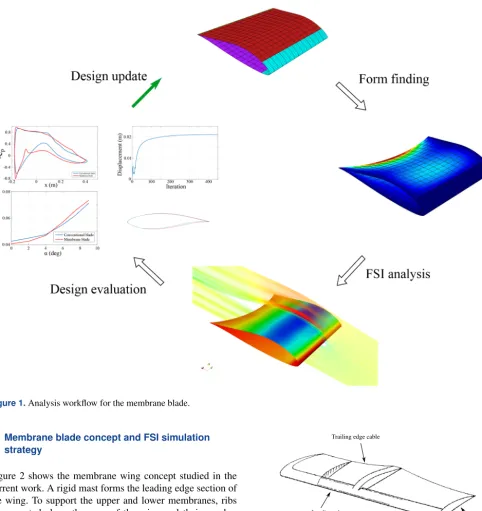
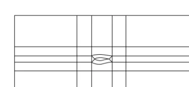
Analysis of the membrane blade consists of three major steps. They are represented in Fig. 1 for a sample section. In the form-finding step, the equilibrium shape in the absence of external loading is calculated, which is the shape at the beginning of an FSI simulation. Then in the FSI analysis, the interaction between the membrane and the fluid flow is sim-ulated. The FSI analysis is followed by evaluating the design in terms of aerodynamic and structural characteristics of the blade. The cycle could be repeated for a new design to realize a better aerodynamic performance of the blade.
The goal of the current contribution is to make a compar-ison between a membrane blade and its conventional rigid-blade counterpart. The NASA-Ames Phase VI rotor (Hand et al., 2001) is chosen as the reference rigid-blade config-uration. The membrane blade uses the same planform as the NASA-Ames Phase VI rotor blade. Along the span, the blade is divided into four segments of equal span. The upper and lower surface of each segment is a prestressed membrane. The membranes are both connected to a prestressed cable at the trailing edge.
Figure 1.Analysis workflow for the membrane blade.
2 Membrane blade concept and FSI simulation strategy
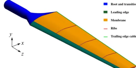
Figure 2 shows the membrane wing concept studied in the current work. A rigid mast forms the leading edge section of the wing. To support the upper and lower membranes, ribs are mounted along the span of the wing and their number depends on the span length of the wing. Upper and lower membranes are joined together at the trailing edge via a pre-tensioned edge cable.
In the case of a flexible membrane blade, the shape of the blade’s surface depends on the one hand on the working con-ditions in terms of wind speed, angle of attack, etc., and on the other hand on the structural properties of its supporting frame and the membranes which form the wing surface. The pressure distribution on the surface of the wing depends on the form and the above-mentioned working condition. The structural properties of the wing govern its deformation un-der such a loading. The final form of the wing results from this interaction between loading and displacement. This
em-Rib Leading edge mast
Trailing edge cable
Figure 2.Sailwing construction concept from Ormiston (1971).
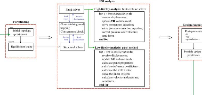
The analysis starts with a form-finding simulation. In form finding, the equilibrium state of the wing is calculated; i.e. the state in which membrane and edge cable internal forces are in equilibrium is computed. This is the initial shape of the blade surface in the absence of external forces. FSI sim-ulations are started from this initial state. In the following sections, fluid, structure, and coupling-related aspects are ex-plained in detail. The overall simulation work flow is shown in Fig 3, which demonstrates the sequence of the simulations. The process of solving the flow problem for both ap-proaches is presented in the figure as well. At each coupling iteration the fluid solver receives the displacement from the structural solver and updates the mesh. Then the fluid prob-lem is solved for the updated mesh. It should be noted that in solving the problem using the finite-volume method, all the steps include operations performed on a three-dimensional mesh, while in the panel method the mesh consists of two-dimensional surface discretization. In the case of the mesh update in particular, for the panel method discretization up-dating the mesh means adding the displacement at each node to the original coordinate of the node, but for the three-dimensional volume mesh, in addition to applying the dis-placement on the boundary the disdis-placement of the interior points should also be calculated. In addition to the higher computational cost of the three-dimensional mesh morphing, it is also a challenge to keep the quality of the volume ele-ments as they deform.
2.1 Fluid model
Two approaches of very different fidelity are used for the modelling and simulation of fluid flow. The first one is the finite-volume-based numerical solution of Navier–Stokes equations using OpenFOAM and the second one is the vortex panel method. The advantage of the vortex panel method is that it is computationally less demanding, while its drawback is that it neglects the viscous effects. Still it is a very good alternative to Navier–Stokes during the early design stages. While a steady-state FSI simulation using the first approach takes about 10 h to converge, the same simulation takes about 20 min to converge to the steady-state solution using the vor-tex panel method (the same machine (3.40 GHz, 8 M Cache, 15 GB RAM) was used for both approaches). Even though some details of fluid flow are neglected in the vortex panel method, the fact that it is much faster than solving Navier– Stokes equations enables design space explorations at rea-sonable computational costs in a certain range of operating conditions.
2.1.1 Navier–Stokes equations
The Navier–Stokes equations are the general equations de-scribing the flow of fluid substances. For incompressible fluid flow with constant viscosity and density they read
∇ ·(ρv)=0 (1)
and
ρ(∂v
∂t +v· ∇v)= −∇p+µ∇
2v+f. (2)
Velocity (v) and pressure (p) fields are coupled in these
equations. The SIMPLE algorithm of Patankar and Spalding (Patankar and Spalding, 1972) is used to enforce the cou-pling. A Reynolds-averaged Navier–Stokes model is used for turbulence modelling, and turbulent viscosity is modelled
us-ing ak−ωSST model (Menter, 1994). It is a two-equation
model used to calculate the kinematic eddy viscosity. First
the equations for turbulent kinetic energy (k) and specific
dis-sipation rate (ω) are solved. Kinematic eddy viscosity is then
calculated fromk,ω, and other parameters of the model.
Near the no-slip boundaries, normal gradients become larger as the distance to the wall tends to 0 and viscous ef-fects become more important. Usually the region near the wall is not directly resolved via the numerical model, but the so-called law of the wall, also known as wall function, is used to model the flow behaviour in this region. At the blade’s sur-face, OpenFOAM wall functions are used: the
kqRWallFunc-tion forkand omegaWallFunction forω. The wall functions
set their corresponding parameter,ωork, for the first node
in the normal direction to the boundary. The boundary
condi-tion is set based on the logarithmic law ify+>11.5 and the
linear law ify+<11.5.
Fluid solver
-N on-matching mesh mapping -Convergence check FSI analysis Design evaluation Post-processing: - CL - CD - cp distribution, ...
Possible update in prestresses
Receive displacement
-initial topology -prestresses
E quilibrium shape
Formfinding
I nput
O utput
for i = 0 to maxIteration do
receive displacement; update 3D volume mesh; solve momentum equation; solve pressure correction equation; correct pressure and velocities; send force
end for
for i = 0 to maxIteration do
receive displacement; update 2D volume mesh; calculate panel properties; calculate influence coefficients; calculate the RHS vector; solve the linear system; calculate velocity and pressure; send force
end for
High -fidelity analysis: finite-volume solver
Low- fidelity analysis: panel method Structural solver Send force Send displacement Receive force
Figure 3.Schematic representation of the multi-fidelity analysis work flow.
2.1.2 Vortex panel method
The velocity field for the case of irrotational, incompressible, and inviscid flow can be represented by a velocity potential
8. This is the basis for the vortex panel method. The flow
velocity can be calculated from the potential in the following way:
u= −∂8
∂x, (3)
v= −∂8
∂y, (4)
w= −∂8
∂z. (5)
Inserting the above equations into continuity Eq. (1) results in the continuity equation in terms of the potential:
∇28=0. (6)
This equation can be solved by the superposition of elemen-tary solutions. There are two boundary conditions for solving this Laplacian equation. One is that for a body submerged in fluid, the velocity component normal to the body’s surface should vanish:
∇8·n=0, (7)
wherenis the vector normal to the surface. The other
con-dition is that the disturbance in the free-stream flow caused
by the elementary solutions should vanish as the distance,r,
from the boundary surface increases:
lim
r→∞∇8=0. (8)
Using Green’s identity, it can be shown that the potential
at each point,P, inside the domain can be calculated in terms
of the potential (8) and its derivative (∂8∂n) on the boundary
of the domain:
8(P)= 1
4π
Z
S
(1
r∇8−8∇
1
r)·ndS. (9)
A detailed derivation of Eq. (9) is available in Katz and Plotkin (2008). The problem is now reduced to finding the values of the potential on the boundary which fulfill the con-tinuity Eq. (6) and the two boundary conditions stated in Eqs. (7) and (8). The Laplace equation is a linear equation and if two functions fulfill the equation, their linear combi-nation fulfills the equation as well. Hence, the solution of the continuity equation can be found as a superposition of ele-mentary solutions like sources and doublets on the boundary of the domain.
In the panel method the strength of these singular solutions is calculated using the boundary condition stated in Eq. (7) to enforce zero normal velocity at the surface of the bound-ary. The surface of the wing is discretized with a number of panels as shown in Fig. 4. Each panel on the wing surface represents a quadrilateral source and a quadrilateral doublet element. In addition to wing panels there are wake panels to represent the wake behind the wing. Wake panels consist of quadrilateral doublets.
The Dirichlet implementation of the zero normal flow boundary condition is used for the collocation point at each panel. The collocation point of a panel is at the centre of the panel (in the case of the Dirichlet boundary condition the collocation points are infinitesimally shifted inside the body).
The velocity at collocation pointP is calculated by summing
up the contribution of each panel to the velocity at this point:
v(P)=
N X
k=1
Ckµk+ Nw
X
l=1
Clµl+ N X
k=1
Figure 4.Discretization of the wing surface into panels from Katz and Plotkin (2008).
whereN is the number of panels on the wing’s surface and
Nwis the number of wake panels. The first term in Eq. (10)
is for the contribution of doublet elements on the wing panel, the second represents the contribution of doublet element at the wake, and finally the last one is for source terms on the
wing.Ck can be interpreted as the velocity caused by thekth
panel at pointP; it is calculated for a panel of unit strength.
The same interpretation holds for Bk regarding the source
terms. For more details on the calculation of the influence
co-efficientsCkandBk, we refer the reader to Katz and Plotkin
(2008). The total velocity at pointP is the velocity caused
by the panels plus the free-stream velocity. To set the total velocity in the normal direction to the panel to zero, the con-tribution of panels should cancel out that of the free-stream velocity:
N X
k=1
Ckµk+ Nw
X
l=1
Clµl+ N X
k=1
Bkσk !
·n= −v∞·n. (11)
Equation (11) should hold at every collocation point. Apply-ing this equation to each collocation point, we end up with
a system ofN equations withN unknowns. This system of
linear equations is then solved for the unknowns, which are the strengths of the doublet panels. It should be mentioned
that the strength of thekth source panels is already set to
σ(k)=v∞·n(k), (12)
where v∞ is the free-stream velocity and is moved to the
right-hand side before solving the system of linear equations.
In Eq. 12,v∞is the free-stream velocity vector. The strength
of wake panels is also calculated in terms of doublet strength at the upper and lower neighbouring panels of the trailing edge (Fig. 5) using the Kutta condition.
The Kutta condition implies that the circulation at the trail-ing edge should be zero. Three panels intersect at the trailtrail-ing edge. These are the wake panel and the two wing panels on
Figure 5.Wake panels used to apply the Kutta condition from Katz
and Plotkin (2008).
0.2 0.4 0.6 0.8 1
−1 −0.5 0
0.5
1
1.5
2
x/c
−
cp
XFLR5
Panel method
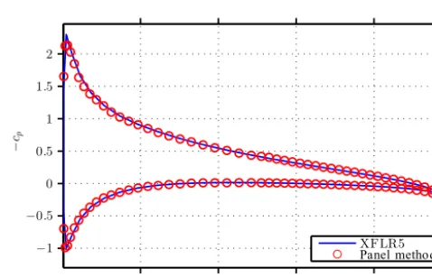
Figure 6.Pressure distribution over a NACA0012 wing section,
α=6◦.
the upper and lower surface of the wing. The Kutta condi-tion is satisfied by setting the difference in the strength of the upper and lower panel to the wake strength:
µw=µupper−µlower. (13)
Strength of the doublet panels are calculated by solving the resulting system of linear equations. In the post-processing step the velocity at the points of interest, which are the collo-cation points in particular, is calculated. The pressure is then calculated from the steady-state Bernoulli equation.
Figure 6 shows the calculated pressure distribution in the middle section of a NACA0012 wing for an angle of attack
of 6◦. The results are compared with the ones from XFLR5
to check the correctness of the developed panel solver which is used in the remainder of this publication as a low-fidelity fluid solver.
2.2 Structural model
anal-P oint support
P restressed edge cable
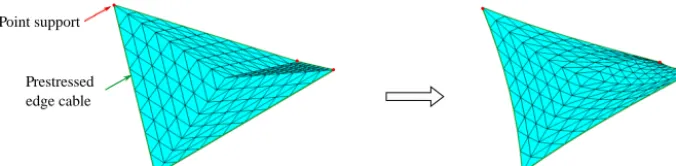
Figure 7.Form-finding analysis of a four-point tent. Left: initial state. Right: equilibrium state.
ysis. In general, structural analysis of membranes using the finite-element method is used and displacements are calcu-lated for a specific structure under an applied load. Form finding of membrane structures can be seen as the inverse problem of structural analysis. Prestressed membrane struc-tures can be supported at the edges by pretensioned edge ca-bles. In the inverse problem of form-finding, the stresses in membrane and edge cables are given and support conditions (fixed boundaries) are defined. The goal of the form-finding analysis is to find the shape at which an equilibrium between structural forces exists. In other words, form-finding analysis calculates the equilibrium shape of the membrane enclosed by a given boundary and with predefined stress distributions. It has been inspired, e.g., by the works of the German ar-chitect, Frei Otto (Otto and Rasch, 1995) and was originally developed for form finding of cable structures. Form finding could be done using different approaches like the force den-sity method (Schek, 1974), dynamic relaxation (Wakefield, 1999), or the updated reference strategy (URS) (Bletzinger and Ramm, 1997; Wüchner and Bletzinger, 2005). We have used the URS-based method available in the in-house struc-tural solver CARAT++. As a classical form-finding example, the four-point tent is presented in Fig. 7. The reference con-figuration of the four-point tent example consists of four flat membrane patches. They are connected to four edge cables at the boundaries and are fixed at four support points. After ap-plying prestresses to the four membranes and the supporting edge cables, the structure evolves from flat membranes to a double curved surface where internal membrane prestresses are in equilibrium with the forces from the four edge cables. CARAT++ has also been used for performing static non-linear finite-element method (FEM) analysis using the load-control method. This starts from the equilibrium state and computes the deformations due to the external loads caused by the fluid flow.
2.3 Fluid-structure interaction
Fluid–structure interaction studies the interactions between a solid body and its surrounding fluid. The interface between
the fluid field (F) and the structure field (S) is designated
by0I. The load from the fluid field is coupled with the
dis-placement from the structure field. There are two coupling conditions enforced at the interface:
2.3.1 Kinematic continuity condition
Enforcing this constraint ensures that the fluid and structure interfaces lie on each other during the simulation. It is satis-fied if the displacement at the fluid interface is the same as the displacement at the solid interface:
dF0
I(t)=d
S
0I(t). (14)
2.3.2 Dynamic continuity condition
Dynamic continuity condition is about mapping the correct force vector from the fluid interface to the solid interface. It implies
fF0
I(t)=f
S
0I(t). (15)
The interface mesh at the fluid side is in most cases finer than the mesh at the structure side. Non-matching mesh mapping techniques are necessary to map the equivalent nodal force and nodal displacement at the FSI interface. A mortar map-ping method is used in the current work. A basic criterion for mapping algorithms is consistency. It implies that a constant field is mapped exactly from one mesh to the other mesh. An-other criterion is the conservation of energy, which is used to derive the so-called conservative mapping operators. In con-servative mapping, total energy is conserved as the fields are mapped between the meshes at the interface. The conserva-tion of interface energy reads
Z
0
dF0TfF0d0=
Z
0
dS0TfS0d0. (16)
Normal and dual mortar algorithms for mapping are not con-sistent in general. A novel technique for enforcing consis-tency on the mapping algorithm by scaling up the structural shape functions for the calculation of mapping matrices is utilized. For the details of the formulation and its implemen-tation, we refer to Wang et al. (2016).
Ω
FΩ
FΩ
SΩ
S1
2
3
4 dΓ
n
dΓn+1
n+1
fΓ
n n+1
I
I I
Figure 8.Solution procedure for the coupled problem.
is divided into two separate sub-problems for fluid and struc-ture field (Wüchner et al., 2007). Each field is solved sepa-rately in the partitioned approach and the exchange of infor-mation takes place in a separate coupling step. The mono-lithic approach typically has an advantage over the parti-tioned one in terms of stability and accuracy (Kupzok, 2009). On the other hand, solving the two fields independently in a modular environment provides the possibility of using the most efficient available solution techniques for each field. Thus, this is the preferred simulation approach to develop the multi-fidelity analysis concept.
For a steady-state FSI simulation, the coupling steps in each iteration are as follows:
1. Solve the fluid problem for the new iteration (n+1).
2. Send the resulting force at the interface to the structure solver.
3. Solve the structure problem.
4. Send the calculated displacement to the fluid solver and proceed to the next iteration.
Schematic representation of these steps is shown in Fig. 8. In the following the structure problem is abbreviated by
the operatorSand the fluid problem by the operatorF. On
the structure side the solver receives the loading from the fluid solvers and calculates the displacement at the interface:
dn0+1
I =S(f
n+1
0I ). (17)
For the fluid solver it is just the opposite; it receives the dis-placement at the interface and delivers the load applied by the fluid:
fn0+1
I =F(d
n
0I). (18)
Insertingd0 from Eq. (17) into Eq. (18), we have
dn0+1
I =S(f
n+1 0I )=S
F(dn0+1
I )
=S◦F(dn0
I). (19)
Equation (19) could be solved either using fixed-point iteration-based methods or Newton-based methods. In the
Root and transition region
Leading edge
Membrane
Ribs
Trailing edge cable x
y
z
Figure 9.Blade planform.
current work, the Gauss–Seidel method is used to solve the equation iteratively. The convergence of the iterative solution procedure is checked during the iteration steps by comparing the current solution with the previous solution. A relative
tol-erance of 10−6is used as the convergence criterion.
Table 1.Membrane properties (u: upper; l: lower).
E 84 MPa
ρ 1400 kg m−3
t 0.48 mm
σchordwiseu 180 kPa
σspanwiseu 480 kPa
σchordwisel 180 kPa
σspanwisel 480 kPa
Table 2.Trailing edge cable properties.
E 125 GPa
ρ 7800 kg m−3
radius 4 mm
σ 30 MPa
Table 3.Rib properties.
E 190 GPa
ρ 7800 kg m−3
A 2 cm×12 cm
3 Model set-up and results
Top view
U ndeformed
D eformed
D isplacement contour
D eformed U ndeformed
Section view
Figure 10.Form finding of the membrane blade. Undeformed and deformed geometry from top and front views.
Undeformed Deformed
Figure 11.Form finding of the membrane blade (mid-span section,
second segment from the root).
airfoil profile) to 0.35 m at the tip of the blade. Upper and lower membranes are wrapped around the rigid leading edge, which extends up to 15 % of the chord length. The mem-branes are supported by four ribs and by an edge cable at the trailing edge. The four ribs divide the blade into four seg-ments with equal span. The structural properties of the mem-branes, ribs (which are modelled as beams), and edge cable are summarized in Tables 1–3. The prestresses in Table 1 are for the first blade section from the root. The prestress in span
Figure 12.Blocking structure for the fluid mesh.
direction is the same for all four segments, since they all have the same span, but the prestress in chord direction is scaled with the mean chord length for the three other segments.
3.1 Form finding
Inlet Outlet Side walls Blade
Figure 13.Left: fluid domain. Right: fluid mesh in the vicinity of
the blade.
Figure 14.Detailed view of the fluid mesh at the leading edge and
the trailing edge.
toward the leading edge with maximum displacement at the middle of each blade segment. The prestresses in the mem-branes form double-curved membrane surfaces, where the upper membranes are moved downwards and lower mem-branes are moved upwards. While the cross section remains unchanged at the four ribs, due to the deformation of the two membranes, the cross section of the blade changes continu-ously on other sections along the span. Figure 11 shows how the cross section at the middle of the second segment from the root deviates from the initial cross section (which is the S809 airfoil profile) and how the upper and lower membrane pull the elastic trailing edge cable toward the leading edge.
3.2 Fluid set-up
For the fluid side, simpleFoam solver from OpenFOAM has been used for performing steady-state computational fluid dynamics (CFD) simulations. The schematic representation of the blocking strategy is presented in Fig. 12. The com-putational domain together with the mesh in the vicinity of the blade is shown in Fig. 13. For a better presentation of the used mesh, detailed view of the elements structure at the leading edge and the trailing edge is shown in Fig. 14.
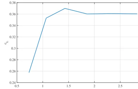
The domain size is 15 m×15 m×45 m, which results in
a blockage ratio of about 0.3 %. The tip of the blade has a distance of 10 m to the far-field boundary. The domain is
discretized with a total of 2.9 million cells (hexahedral and
0.5 1 1.5 2 2.5 3
N umber of elements ×106
0.24 0.26 0.28 0.3 0.32 0.34 0.36 0.38
cL
Figure 15.Mesh convergence study for the rigid blade,α=4.0◦.
tetrahedral elements), which results in a maximumy+value
of about 70. Figure 15 presents the result of the mesh con-vergence study performed for the rigid-blade configuration
atα=4.0◦. As can be seen,cLhas converged for the mesh
with 2.9 million elements.
Thek-ωSST model has been used. OpenFOAM wall
func-tions are used at the blade’s surface: kqRWallFunction fork
and omegaWallFunction forω. The velocity at the inlet is
30 m s−1. The boundary conditions for fluid simulation are
summarized in Table 4.
3.3 FSI simulations
FSI simulations were done for six different angles of attack
from 0 to 9◦. In the following, FSI_CFD is used for
sim-ulations using the finite-volume method on the fluid side and FSI_Panel is used for simulations which use the panel method for flow modelling. Because of blade’s deformation in FSI simulations, the fluid solver should, in addition to solving the fluid flow problem, take care of the movement in the mesh as well. For the FSI_CFD case the deformation of the blade, which is applied to the blade patch, is diffused into the fluid domain. This means that the boundary motion is distributed into the volume mesh and the zero displace-ment condition is applied at the far-field boundaries of the fluid domain. To solve the mesh motion problem the dis-placement Laplacian-based solver from OpenFOAM is used with the quadratic inverse distance diffusion method.
Convergence to the steady-state solution when using the panel method solver is about 30 times faster than using the simpleFoam solver from OpenFOAM as the fluid solver. The panel code was run on a single processor, while for Open-FOAM simulations, 10 processors were used. For both cases
a relaxation factor of 0.15 was used for the displacement field
for all angles of attack except for α=7.5◦ andα=9.0◦,
where the relaxation factor was reduced to 0.1 to improve
stability in the FSI run. The relaxation factor (ωr) is applied
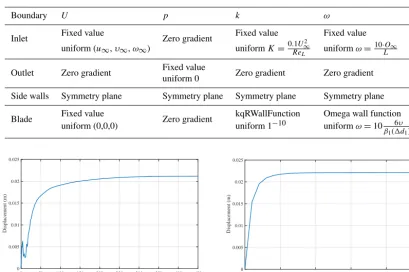
Table 4.Boundary conditions for computational fluid dynamics (CFD) simulations.
Boundary U p k ω
Inlet Fixed value Zero gradient Fixed value Fixed value
uniform (u∞,υ∞,ω∞) uniformK=0.1U
2
∞
ReL uniformω=
10·O∞
L
Outlet Zero gradient Fixed value Zero gradient Zero gradient
uniform 0
Side walls Symmetry plane Symmetry plane Symmetry plane Symmetry plane
Blade Fixed value Zero gradient kqRWallFunction Omega wall function
uniform (0,0,0) uniform 1−10 uniformω=10 6υ
β1(1d1)2
0 50 100 150 200 250 300 350 400 450
I teration
0 0.005 0.01 0.015 0.02 0.025
D isplacement (m)
0 5 10 15 20 25
I teration
0 0.005 0.01 0.015 0.02 0.025
D isplacement (m)
Figure 16.Convergence of the displacement for the selected monitor point. Left: FSI_CFD. Right: FSI_Panel.
Table 5.Comparison of displacement (m) inydirection for
differ-ent angles of attack.
α(deg) FSI_Panel FSI_CFD %diff
0.0 0.0175 0.0170 2.87
2.0 0.0198 0.0189 4.74
4.0 0.0221 0.0211 4.73
6.0 0.0241 0.0231 4.38
7.5 0.0252 0.0241 4.53
9.0 0.0255 0.0237 7.68
fluid solver in increments but to send a fraction of that to im-prove the stability of the coupling algorithm and preserve the quality of the mesh on the fluid side:
dn0+1
I,sent=ωrd
n+1
0I,calculated+(1−ωr)d
n
0I. (20)
The relaxation factor should be kept below a certain limit (which is case dependent) for FSI_CFD simulations, other-wise the quality of the finite-volume mesh cannot be pre-served during the simulation and the simulation might crash as a result of having highly distorted elements in the mesh. The same relaxation factor is used for the FSI_Panel case. The reason for using the same relaxation factor is to have a fair comparison between the convergence behaviour of the two approaches, but it must be mentioned that for FSI_Panel
cases a higher relaxation factor can be used as well to have faster convergence without getting stability problems due to distorted element in the mesh, which in this case is just a discretized surface.
First, we compare the convergence behaviour of the dis-placements to the steady-state solution for each approach (Fig. 16). Displacement of the point in the mid-span
sec-tion of the second segment from the root withx / c=0.5
is compared (c is the chord length). While with the panel
method convergence is reached within 25 iterations, FSI sim-ulation using simpleFoam takes 450 iterations to converge. The time each iteration takes is also different in the two ap-proaches. Overall, in the case of the panel method, conver-gence is reached approximately 30 times faster. For this par-ticular case, the FSI_CFD simulation has taken about 10 h to converge using 10 processors, but FSI_Panel has
con-verged within about 20 min on a single processor. Forα=4◦
the converged displacement is 0.0221 m from FSI_Panel and 0.0211 m from FSI_CFD, which demonstrates clearly the applicability of the low-fidelity approach, provided that the blade-operating condition is in agreement with the respective modelling assumptions (see Sect. 2.1.2).
The comparison of the two approaches for the selected
monitor point is summarized in Table 5. For α=0◦ the
difference in the calculated displacement from the two
ap-proaches is 2.87 %. The difference increases with the angle
α= 0.0° α= 2.0°
α= 4.0° α= 6.0°
α= 9.0° α= 7.5°
FSI_CFD FSI_Panel method
Figure 17.Comparison of the converged cross section in the mid-span section of the second segment from the root.
0 2 4 6 8 10
α(deg) 0.04
0.05 0.06 0.07 0.08
cD
Conventional blade Membrane blade
0 2 4 6 8 10
α(deg) 0
0.2 0.4 0.6 0.8 1
cL
Conventional blade Membrane blade
0 2 4 6 8 10
α(deg) 0
2 4 6 8 10 12
L/D
Conventional blade Membrane blade
Figure 18.Comparison between the aerodynamic characteristics of the membrane blade and rigid blade.
profile, stall happens atα≈9◦. With the emergence of stall
and flow separation, the assumptions of the panel method are no more valid. This explains the increased deviation of the
FSI_Panel result from the FSI_CFD result forα=9◦.
After local comparison of the calculated displacements for the two approaches in Table 5 for a single monitor point, a more global comparison is made by comparing the converged cross section shape in the steady state. Figure 17 shows the cross section of the blade in the middle of the second segment from the root. For the upper surface of the blade, there is a good agreement between the two methods, even though the difference increases with the angle of attack, which is to be expected. The difference in the converged shape is higher for
the lower surface and especially forα=7.5◦andα=9.0◦. It
can be explained by the increased discontinuity in the slope of the surface at the point at which the lower membrane is attached to the leading edge mast. At the point of attachment there is a kink, which is much more visible for higher angles of attack. The local flow separation downstream of the kink is not captured by the panel method, which results in dif-ferent pressure distributions and as a consequence difdif-ferent converged shapes for the two approaches.
-0.2 -0.1 0 0.1 0.2 0.3 0.4 0.5
x (m) -0.015
-0.01 -0.005 0 0.005 0.01 0.015 0.02
y
(m
)
S809
α= 0°
α= 4°
α= 6°
α= 9°
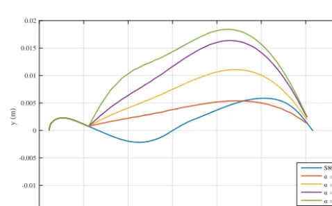
Figure 19.Comparison of the camber line in the middle span
sec-tion of the second segment from the root.
Table 6.Percentage change in aerodynamic characteristics of the membrane blade compared with the rigid blade.
α(deg) 0.0 2.0 4.0 6.0 7.5 9.0
1cL −75.5427 −12.4708 7.4925 15.0273 17.6614 13.9290
1cD −4.2353 −5.3452 −1.4706 3.4483 5.9390 2.9494
1(L / D) −74.4610 −7.5280 9.0968 11.1931 11.0652 10.6650
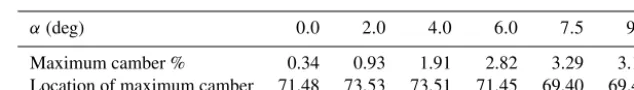
Table 7.Maximum camber and its location for the middle span section of the second segment from the root.
α(deg) 0.0 2.0 4.0 6.0 7.5 9.0
Maximum camber % 0.34 0.93 1.91 2.82 3.29 3.17
Location of maximum camber 71.48 73.53 73.51 71.45 69.40 69.40
-0.2 -0.1 0 0.1 0.2 0.3 0.4 0.5
x (m) -0.8
-0.6 -0.4 -0.2 0 0.2 0.4 0.6 0.8 1
-cp
Conventional blade Membrane blade
Figure 20.Pressure coefficient distribution over the middle span
section of the second segment from the root.
rigid-blade configurations in stall region because of the so-called “soft stall characteristics” of the membrane wings (Maughmer, 1979). In order to assess the aerodynamic per-formance of the studied blade, the lift coefficient, drag coeffi-cient, and lift-to-drag ratio of the blade are compared with the rigid-blade configuration (i.e. the configuration before form finding). As can be seen in Fig. 18, for smaller angles of at-tack the membrane blade has smaller lift and drag coefficient compared with the rigid blade; however, with the increase in the angle of attack, higher lift and drag coefficients are observed for the membrane blade. Table 6 provides a nu-meric comparison of the change in these coefficients com-pared with the rigid blade. The cross section of the membrane blade in the absence of an aerodynamic load is shown in Fig. 11 (the orange curve). The membrane blade has a pretty
much symmetric profile in the unloaded state. Forα=0.0◦,
the converged cross section is also a rather symmetric profile (Fig. 17). This explains the big decrease in the lift coefficient
of the membrane blade atα=0.0◦, compared with the rigid
blade with the asymmetric S809 airfoil. With the increase in the angle of attack, the loading on the blade, and as a con-sequence the converged cross section profile, becomes more
and more asymmetric, which can be seen in Fig. 17. More-over the displacements in the membranes increase with the increase in the angle of attack. It increases the thickness of the blade profile and as a consequence there is an improve-ment in the lift coefficient of the membrane blade compared with the rigid blade for higher angles of attack. The drag coefficient increases as well with the increase in the angle of attack and the drag coefficient of the membrane blade is higher than that of the rigid blade. But the improvement in the lift coefficient is larger compared with the increase in the
drag coefficient, and consequently forα=4.0◦ and higher
angles of attack the lift-to-drag ratio for the membrane blade is higher compared with the conventional rigid blade. While having a higher lift coefficient and lift-to-drag ratio is not desired for a stall-controlled turbine like the NASA-Ames Phase VI rotor, it should be mentioned that the purpose of the current study is to investigate the characteristics of the membrane blade concept and make a comparison between the membrane blade and a conventional blade. No conclu-sion could be made at this stage whether the concept should be utilized for pitch-controlled or stall-controlled turbines.
The cross section of the membrane blade varies along the span. Membrane deformation changes the cross section prop-erties of the blade like the maximum camber and thickness. The original S809 airfoil has a maximum camber of about
1 % at 82.3 % chord position, but for the membrane blade,
the maximum camber and its location changes with the an-gle of attack (Table 7). It is also shown in Fig. 19 that with the increase in the angle of attack the maximum camber in-creases as well, and in general the point of maximum camber moves slightly towards the leading edge of the blade.
The increase in the lift coefficient for the membrane blade could also be seen in the pressure coefficient distribution over the blade’s surface. The pressure coefficient distribution over the middle span section of the second segment from the root is plotted in Fig. 20 and is compared with the pressure
coeffi-cient distribution of the rigid blade forα=6.0◦. The kink in
where the lower membrane is attached to the rigid leading edge mast.
4 Conclusion
Fluid-structure interaction simulation of a semi-flexible membrane blade configuration is done over a range of angles of attack. Two different fluid models were used: CFD simula-tion based on RANS equasimula-tions and the vortex panel method. The panel method saves computation time while providing
a good accuracy up to an angle of attack of 6◦. This makes
the panel method an appropriate tool for early design stages of the membrane blade where an extensive parameter study needs to be done. Its accuracy could be improved by coupling boundary layer models with it. Comparing the performance of the membrane blade with its representative rigid counter-part the following main observations are made:
1. A higher lift curve slope for the membrane blade is ob-served. Even though the membrane blade has a smaller lift coefficient at zero angle of attack than the rigid blade, due to the higher slope of the lift curve, the mem-brane blade shows a higher lift coefficient compared with the rigid blade.
2. With the increase in the angle of attack, the lift-to-drag ratio of the membrane blade becomes higher than that of the rigid blade.
3. The maximum camber and its location for a membrane blade depends on the angle of attack. The maximum camber of the membrane blade is higher than the rigid blade. With the increase in the angle of attack, there is a slight shift of the point of maximum camber toward the leading edge.
Acknowledgements. The support provided by the Deutsche
Forschungsgemeinschaft (DFG) (BL 306/32-1) is gratefully acknowledged.
Edited by: G. J. W. van Bussel
Reviewed by: A. Vire and two anonymous referees
References
Abdulrahim, M., Garcia, H., and Lind, R.: Flight Characteristics of Shaping the Membrane Wing of a Micro Air Vehicle, J. Aircraft, 42, 131–137, doi:10.2514/1.4782, 2005.
Baumgärtner, D., Wolf, J., Rossi, R., Wüchner, R., and Dadvand, P.: Contribution to the Fluid-Structure Interaction Analysis of Ultra-Lightweight Structures using an Embedded Approach, In-ternational Center for Numerical Methods in Engineering, Vol. CIMNE Monograph M152, 2015.
Barbarino, S., Dettmer, W., and Friswell, M.: Morphing Trailing Edges with Shape Memory Alloy Rods, ICAST, 4–6 October, State College, PA, USA, 2010.
Barlas, A. K., Tibaldi, C., Zahle, F., and Madsen, H.: Aeroelas-tic Optimization of a 10 MW Wind Turbine Blade with Ac-tive Trailing Edge Flaps, 34th Wind Energy Symposium, AIAA, doi:10.2514/6.2016-1262, 2016.
Bletzinger, K.-U. and Ramm, E.: A General Finite Element Ap-proach to the form Finding of Tensile Structures by the Updated Reference Strategy, Int. J. Space Struct., 14, 131–145, 1999. Blondeau, J., Richeson, J., and Pines, J. D.: Desing,
develop-ment and testing of a morphing aspect ratio wing using an inflatable telescopic spar, 44th AIAA/ASME/ASCE/AHS/ASC Structures, Structural Dynamics, and Materials Conference, doi:10.2514/6.2003-1718, 2003.
Bottasso, C. L., Croceb, A., Gualdonib, F., and Montinarib, P.: Load mitigation for wind turbines by a passive aeroe-lastic device, J. Wind Eng. Ind. Aerod., 148, 57–69, doi:10.1016/j.jweia.2015.11.001, 2016.
Bowmann, J., Sanders, B., Cannon, B., Kudva, J., Joshi, S., and Weisshaar, T.: Development of Next Generation Morphing Aircraft Structures, 48th AIAA/ASME/ASCE/AHS/ASC Struc-tures, Structural Dynamics, and Materials Conference, Honolulu, Hawaii, doi:10.2514/6.2007-1730, 2007.
Fink, M.: Full-scale Investigation of the Aerodynamic Characteris-tics of a Model Employing a Sailwing Concept, NASA-TN-D-4062, 1967.
Fink, M.: Full-scale Investigation of the Aerodynamic Characteris-tics of a Sailwing of Aspect Ratio 5.9, NASA-TN-D-5047, 1969. Hand, M., Simms, D., Fingersh, L., Jager, D., Cotrell, J., Schreck, S., and Larwood, S.: Unsteady aerodynamics experiment phase VI: wind tunnel test configurations and available data campaigns, Technical Report NREL/TP-500-29955, NREL, Golden, CO, USA, 2001.
Jasak, H.: Dynamic Mesh Handling in OpenFOAM, 48th AIAA Aerospace Sciences Meeting, Orlando, Florida, 2009.
Jasak, H. and Tukovic, Z.: Automatic mesh motion for unstructured finite volume method, T. FAMENA, 30, 1–18, 2007.
Katz, J. and Plotkin, A.: Low Speed Aerodynamics, Cambridge, Cambridge Univ. Press, 2008.
Kupzok, A. M.: Modeling the Interaction of Wind and Membrane Structures by Numerical Simulation, Technical University of Munich, 2009.
Levin O. and Shyy W.: Optimization of a flexible low Reynolds number airfoil, 39th Aerospace Sciences Meeting and Exhibit, Aerospace Sciences Meetings, doi:10.2514/6.2001-125, 2001. Lian, Y. and Shyy, W.: Numerical Simulation of Membrane Wing
Aerodynamics for Micro Air Vehicle Applications, J. Aircraft, 42, 865–873, doi:10.2514/1.5909, 2005.
Maughmer M. D.: Optimization and Characteristics of a Sailwing Windmill Rotor, Princeton University, 1976.
Maughmer, M. D.: A Comparison of the Aerodynamic Charac-teristics of Eight Sailwing Airfoil Sections, Proceedings of the 3rd International Symposium on the Science and Technology of Low Speed and Motorless Flight, Hampton, VA, USA, 155–176, 1979.
Ormiston, R.: Theoretical and Experimental Aerodynamics of the Sailwing, J. Aircraft, 8, 77–84, doi:10.2514/3.44232, 1971. Otto, F. and Rasch, B.: Finding Form, Deutscher Werkbund Bayern,
Edition A, Menges, 1995.
Patankar, S. V. and Spalding, D. B.: A calculation procedure for heat, mass and momentum transfer in three-dimensional parabolic flows, Int. J. Heat Mass Tran., 15, 1787–1806, doi:10.1016/0017-9310(72)90054-3, 1972.
Saeedi, M., Wüchner, R., and Bletzinger, K.-U.: Multi-fidelity Fluid-Structure Interaction Analysis of a Membrane Wing, 17th International Conference on Applied Aerodynamics and Aeromechanics, London, 169–176, 2015.
Schek, H.-J.: The force density method for form finding and com-putations of general networks, Comput. Method. Appl. M., 3, 115–134, doi:10.1016/0045-7825(74)90045-0, 1974.
Valasek, J.: Morphing Aerospace Vehicles and Structures, John Wi-ley, 2012.
Viré, A., Xiang, J., and Pain, C. C.: An immersed-shell method for modelling fluid–structure interactions, Philos. T. R. Soc., 373, 2035, doi:10.1098/rsta.2014.0085, 2015.
Wakefield, D. S.: Engineering analysis of tension structures: the-ory and practice, Eng. Struct., 21, 680–690, doi:10.1016/S0141-0296(98)00023-6, 1999.
Wang, T., Wüchner, R., Sicklinger, S., and Bletzinger, K.-U.: As-sessment and improvement of mapping algorithms for non-matching meshes and geometries in computational FSI, J. Com-put. Mech., 57, 793–816, doi:10.1007/s00466-016-1262-6, 2016. Waszak, R. M., Jenkins, N. L., and Ifju, P.: Stability and Control Properties of an Aeroelastic Fixed Wing Micro Aerial Vehicle, AIAA Atmospheric Flight Mechanics Conference and Exhibit, Guidance, Navigation, and Control and Co-located Conferences, Montreal, Canada, doi:10.2514/6.2001-4005, 2001.
Wüchner, R. and Bletzinger, K.-U.: Stress-adapted numerical form finding of pre-stressed surfaces by the updated refer-ence strategy, Int. J. Numer. Method. Eng., 64, 143–166, doi:10.1002/nme.1344, 2005.