Performance of CCC-r control chart with variable sampling intervals

Vol. 4, No. 2, 2017, pp. 19-34

DOI: 10.22116/JIEMS.2017.54603

www.jiems.icms.ac.ir

Performance of CCC-r control chart with variable sampling

intervals

Mohammad Saber Fallah Nezhad1,*, Yousof Shamstabar1, Mohammad Mahdi Vali Siar2

Abstract

The CCC-r chart is developed based on cumulative count of a conforming (CCC) control chart that considers the cumulative number of items inspected until observing r nonconforming ones. Typically, the samples obtained from the process are analyzed through 100% inspection to exploit the CCC-r chart. However, considering the inspection cost and time would limit its implementation. In this paper, we investigate the performance of CCC-r chart with variable sampling interval (CCC-rVSI

chart). The efficiency of CCC-rVSI chart is compared with fixed sampling interval (FSI) scheme of

CCC-r chart (CCC-rFSI chart) and CCCVSI chart. The comparison results show that CCC-rVSI chart is

more efficient than the CCCVSI chart in reducing the average time to signal (ATS) and also CCC-rVSI

chart performs better than CCC-rFSI chart. In addition, some sensitivity analyses are performed to

illustrate the effect of the input parameters on the performance of CCC-rVSI chart.

Keywords: Attribute control chart; variable sampling interval; CCC-r chart; average time to signal

Received: July 2017-11 Revised: October 2017-06 Accepted: December 2017-06

1.

Introduction

Attribute control chart is a tool for statistical process control (SPC) that is applied for increasing stability and improving quality through variability reduction in the production process. The cumulative count of conforming (CCC) control chart is a type of attribute control chart that is based on the cumulative number of conforming items between two consecutive nonconforming items and follows the geometric distribution (Calvin, 1983; Goh, 1987). It is useful for high-quality process like automated manufacturing systems. The extended state of CCC control chart is called CCC-r control chart which considers the cumulative count of conforming items until observing r non-conforming ones, and it is based on the negative binomial distribution (Ohta et al,2001; Kudo et al,2004). CCC chart is based

* Corresponding Author;Fallahnezhad@yazd.ac.ir

1_{Department of Industrial Engineering, Yazd University, Yazd, Iran.}

on the cumulative number of conforming items, but it makes the chart insensitive to process shifts relatively (Chen, 2014). Kuralmani et al. (2002) and Noorossana et al. (2007) proposed the conditional chart which detects the shifts of nonconforming fraction based on the current point and some of the previous ones in order to improve the performance of the CCC control chart .

Utilizing the scheme of variable sampling interval (VSI) that varies the next sampling interval between successive samples based on of the current point is another method for improving the sensitivity of the CCC chart (Liu et al. , 2006). The motivation of using variable sampling scheme is to decrease the cost of control chart implementation. Also, this chart detects the changes in nonconforming fraction more quickly than CCC chart with fixed sampling intervals (FSI). The length of sampling interval depends on the process condition in a VSI chart. If there are some alarms which show a change in the process, then a shorter sampling interval should be used and if there is no such signal, then a longer sampling interval will be used. If the current value of the control statistic is near to the target, then a longer sampling interval should be applied next, and a shorter sampling interval should be applied when the current value of the control statistic is near to but not outside the control limits.

A substantial number of researchers have considered VSI control chart in order to improve the performance of charts. X control chart with variable sampling interval was studied by some researchers (see for example, Reynolds et al., 1988; Reynolds and Arnold, 1989; Runger and Pignatiello Jr, 1991; Runger and Montgomery, 1993; Amin and Miller, 1993; Zhang et al., 2012; Lee et al., 2016). Aparisi and Haro (2001), Villalobos et al (2005) and Naderkhani and Makis (2016) considered a VSI multivariate Shewhart chart. Reynolds et al.

2.

Description of the CCC-r

VSI

Chart

2.1. Notations

0

p

the in-control nonconforming fraction,

1

p the out-of-control nonconforming fraction,



the true probability of false alarm,

i

X the cumulative count of items inspected between the (i-1)th nonconforming item and the ith nonconforming item (including the last nonconforming item),

N the number of sampling interval lengths for the CCC-rVSI chart,

j

d

j =1,2,…,n. Sampling interval lengths of the CCC-rVSI chart, , i.e., the time between inspections of two consecutive items (dn<dn-1<…<d2<d1)

d

the sampling interval length of the CCC-rFSI chart,

IL the limits in the CCC-rVSI chart which divide the region between UCL and LCL into n sub-regions I1; I2; . . . ; I n (ILn-1<ILn-2<…<IL1),

Li the sampling interval length which is used to obtain Xi,

ARL

ATS

the average run length, the average time to signal,

ATSV the in-control ATS of the CCC-rVSI chart,

ATSF the in-control ATS of the CCC-rFSI chart, '

V

ATS

The out-of-control ATS of the CCC-rVSI chart,

F

ATS the out-of-control ATS of the CCC-rFSI chart,

I _{improvement factor, defined as} ' '

/

V F

I



ATS

ATS

_,

j

q

the probability that point Xi falls within the region Ijwhen the process nonconforming fraction is p0 ,

j

q

the probability that point Xi falls within the regionIjwhen the process nonconforming fraction is p_1,

2.2. CCC-rVSI control chart

As mentioned before, The CCC–r charts are based on the cumulative count of conforming items until detecting r nonconforming item. Assume a process with nonconforming fraction of p and let X denote the cumulative count of items inspected until the detection of the rth

nonconforming item, then X follows the negative binomial distribution with parameters (r, p)

and the probability mass function of X as is following,

1

( )

(1

)

,

,

1,...,

1

x r r

x

f x

p

p x

r r

r











_

_











The cumulative distribution function of X as is follows,

1

( )

(1

)

1

x

i r r

i r

i

F x

p

p

r

 









_

_











(2)

If the acceptable risk of false alarm is α, then the upper control limit, UCL the central control limit, CL and the lower control limit, LCL of the CCC-r control charts are as following(Xie et al, 2012):

1

0 0

1

(1

)

1

/ 2

1

UCL

i r r

i r

i

p

p

r



  







_

_{ }



_









(3)

(4)

(5)

When a point falls outside the control limits, then the process is considered to be out of control. It is necessary to mention that if a plotted point of the CCC−r chart is above the upper control limit, then we have an improvement in the process. On the other hand, a point below the lower control limit is a signal of process deterioration.

The ARL (average run length) is the average number of points plotted until receiving an out-of-control signal. For the CCC−r charts, ARL can be calculated from Eq. (6), with specified values of nonconforming fraction p≠p0and p=p0 for out of control and in control situations respectively.

1

1

1

(1

)

1

UCL

r i r

LCL

ARL

i

p

p

r













_

_











(6)

ANI is the average number of items inspected until a nonconforming signal occurs, that can be calculated for CCC-rFSI and CCC-rVSI chart by using the following equation:

r ANI ARL

p

 (7)

When the CCC-rVSI chart is applied, then a finite number of interval lengths

1

,

2

,.. .,

n

(

1 2

. .

.

n

)

d d

d d



d





d

are used. These interval lengths should be determined based on the practical conditions of manufacturing processes. The interval limits

1

,

2

,.. .,

n

IL IL

IL

are designed in the CCC-rVSI chart, so that the region between UCL and LCL is divided into n sub-regions

I I

₁

, ,.. .,

₂

I

_n , corresponding to the n different intervals. Thus

following framework is used for sampling from the process,

0 0

1

(1

)

0.5

1

CL

i r r

i r

i

p

p

r

 













_









0 0

1

(1

)

/ 2

1

LCL

i r r

1 1 1 1

2 1 2 2 1

1

, X

(

,

)

, X

(

,

)

.

.

.

, X

(

,

)

i

i

i

n i n n

d

I

IL UCL

d

I

IL IL

L

d

I

LCL IL

  

 





_{ }





 







 



(8)

The sampling interval length, Li that is used for inspection between the (i-1) th nonconforming item and the ith nonconforming item depends on the value of Xi-1. The interval limits

IL IL

₁

,

₂

,.. .,

IL

_n1 can be computed as follows (

F

1is inverse function of the negative binomial distribution with parametersr and p0):

(9)

This scheme continues until the IL values fall between UCL and LCL. It can be elaborated as follows:

(10)

(11)

For example, when n=4; then four different intervals are applied. For implementing the CCC-rVSI scheme, control limits IL1, IL2and IL3 are designed between UCL and LCL, so that the

region (LCL, UCL) is divided into four sub-regions.

1 2 ... 2 1 n n

LCLIL_ IL_  IL IL UCL

1 1

1

(1

1

)

,

1

(1

1 2

...

)

2

n n

2

IL



F



 

q





UCL IL

_



F



    

q

q

q





LCL

1

1 1

1

2 1 2

1

1 1 2

(1

)

2

(1 q

)

2

.

.

.

(1

...

)

2

n n

IL

F

q

IL

F

q

IL

F

q

q

q

Therefore, ATS can be calculated based on the following equations:

F

r

ATS

ANI

d

ARL

d

p



 

 

(12)

1 1 2 2

1 2

....

....

n n V

n

r

d q

d q

d q

ATS

ARL

p

q

q

q









 







(13)

3. Performance comparisons between the CCC-r

VSI

and the CCC-r

FSI

chart

In order to evaluate the efficiency of the CCC-rVSI chart, its performance is compared with the CCC-rFSI chart in this section. Note that the fixed values of nonconforming fraction p0 and acceptable risk of false alarm  are assumed for both the CCCFSI and the CCCVSI chart so that these charts have the same ANI value. In order to compare their ATS values, we opt appropriate design parameters for the CCC-rVSI and the CCC-rFSI chart so that the equation

ATSF=ATSV is satisfied at the in control state. Therefore the CCCVSI chart will be matched to the corresponding CCC-rFSI chart when p=p0 and both of them have the same in-control ATS.

On the other hand, when the process nonconforming fraction changes to

p

₁

( p )



₀ , the values of

ATS

'_F and

ATS

'_V should be compared. The control chart with smaller out-of-control

'

ATS

can detect the shift of nonconforming fraction more quickly.

Let

ATS

_F =

ATS

_V, thus,

1 1 2 2 1 1 2 2

1 2

....

....

....

1

n n n n

n

d q

d q

d q

d q

d q

d q

d

q

q

q



























(14)

Thus, the sampling interval length of the CCC-rFSI chart is adjusted to be equal 1(d =1), then by selecting appropriate value values of

(

d d

₁

,

₂

,...

,

d

_n

)

and

(

q q

₁

,

₂

,...

,

q

_n

)

that satisfy Eq. (14), we can obtain the matched CCC-rVSI and CCC-rFSI chart that have the same in-control value of ATS. Then, when the nonconforming fraction shifts to

p

₁, the performance of the CCC-rVSI chart can be analyzed by computing the value of I, that is the ratio of out-of-control

ATS of the CCC-rVSI and the CCC-rFSI chart:

' ' ' '

1 1 2 2

' ' ' '

1 2

....

....

V n n

F n

ATS

d q

d q

d q

I

ATS

q

q

q

















(15)

When I is less than 1.00, the

ATS

'_Vis less than

ATS

'_F. It indicates that the CCC-rVSI chart performs better than the CCC-rFSI chart. Thus the ratio I is the improvement factor. The smaller values of the improvement factor denote an improvement in the performance of the CCC-rVSI chart.

(16)

3.1. Application of CCC-r charts with variable sampling intervals

We now study the behavior of CCC-rVSI chart based on equal probabilities for each interval:

1 2

1

...

_n

q

q

q

n







 



(17)

By using Eq. (14) and substituting

d



1

, we have,

1 1 2 2 1 2

1

1

d q

d q

....

d q

_{n n}

(

d

d

...

d

_n

)

n







 











 

Thus following equation is obtained,

1 2

...

n

d



d

 

d



n

(18)

In this paper, we used data of Liu et.al (2006) for comparison study. They have assumed

0

0.0027,p 0.0005

   and sampling interval lengths ( ,d d_{1 2},...,d_n) with the fixed value of 1

d  can be chosen as follows:

1 2 1 2 3 1 2 3 4

1 2 3 4 5

2, 1.9, 0.1; 3, 1.9, 1, 0.1; n 4, d 1.9, 1.2, 0.8, 0.1;

n 5, d 1.9, 1.5, 1, 0.5, d 0.1;...

n d d n d d d d d d

d d d

           

     

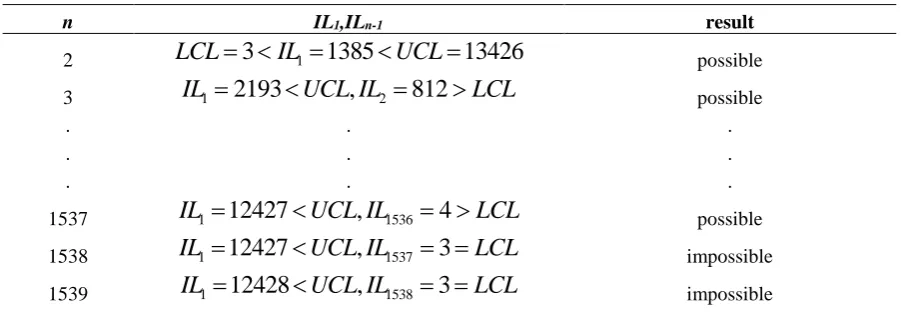
Based on the equations 10 and 11 for each value of the parameter r, possible values for the number of intervals (n) will be obtained. For example in the case CCCVSI (r=1), when

n=1538, the value of IL1537 is equal to LCL according to the equation 11. Thus, this scheme is only possible for the cases n=2, 3,…, 1537. This analysis is denoted in Table 1. Also, the possible value of n can be obtained for other values of r based on constraint (10) and (11).

1 1 2 2 1 1 1

1 1 1

1

2 1 1

1

1 1 1

1 1 1 1

1

(1

)

1

1

(1

)

1

.

.

.

1

(1

)

1

1

(1

)

1

n n n UCL

r x r

x IL

IL

r x r

x IL

IL

r x r

n

x IL

IL

r x r

n

x LCL

x

q

p

p

r

x

q

p

p

r

x

q

p

p

r

x

q

p

p

Table 1. Possible number of intervals (n) for implementing CCCVSI control chart

n IL1,ILn-1 result

2 LCL 3 IL1 1385UCL13426 possible

3 IL12193UCL IL, 2 812LCL possible

. . .

. . .

. . .

1537 IL112427UCL IL, 1536  4 LCL possible 1538 IL112427UCL IL, 1537  3 LCL impossible 1539 IL112428UCL IL, 1538  3 LCL impossible

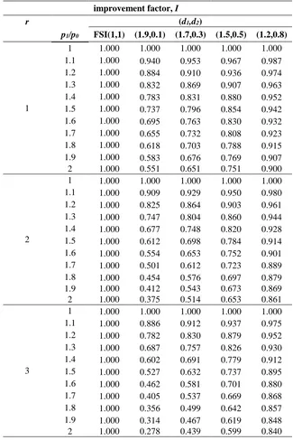
3.2. Improvement factors for different CCC-r control chart based on the number of intervals

In this subsection, by fixing n and based on the assumed parameters in the previous subsection and possible values of r, it is observed that when nonconforming fraction, p1

increases then the improvement factor decreases which demonstrates better performance of CCC-rVSI compared to CCC-rFSI. The results are denoted in Table 2.Also when the parameter r increases, then improvement factor decreases which denotes an improvement in the performance of CCC-rVSI chart. As can be seen in Table 2, (for all values of nonconforming fraction and the parameter r) the values of I are less than 1, thus the performance of CCC-rVSI chart is always better than CCC-rFSI chart.

Table 2. Improvement factors with fixed number of intervals (n=3)

n=3 improvement factor, I

p1/p0 r=1 r=2 r=3 r=4

1 _{1.000 1.000 1.000 1.000}

1.1 0.945 0.917 0.897 0.880

1.2 0.894 0.842 0.802 0.770

1.3 0.848 0.772 0.717 0.673

1.4 0.804 0.709 0.641 0.587

1.5 0.764 0.651 0.573 0.512

1.6 0.726 0.599 0.512 0.448

1.7 0.691 0.551 0.459 0.392

1.8 0.659 0.509 0.413 0.345

1.9 0.629 0.470 0.372 0.305

3.3. Improvement factors for different numbers of sampling intervals

As shown in Table 3, when n=2 and the ratio 1 0

p

p

equals 2, then I = 0.278. It indicates that the CCC-rVSI chart has the best performance in the case n=2 among the other values. Also,

with increasing the ratio 1 0

p

p

the value of I decreases.

Table 3. Improvement factors I for different values of number of intervals

r=3 Improvement factor, I

p1/p0 n=2 n=3 n=4 n=5

1 _{1.000 1.000 1.000 1.000}

1.1 _{0.886 0.897 0.905 0.904}

1.2 _{0.782 0.802 0.819 0.817}

1.3 0.687 0.717 0.741 0.738

1.4 _{0.602 0.641 0.671 0.667}

1.5 _{0.527 0.573 0.608 0.604}

1.6 0.462 0.512 0.552 0.547

1.7 _{0.405 0.459 0.502 0.497}

1.8 _{0.356 0.413 0.458 0.453}

1.9 _{0.314 0.372 0.418 0.413}

2 _{0.278 0.336 0.383 0.378}

3.4. Improvement factors based on different lengths of sampling interval

In this subsection, the number of sampling intervals has been fixed (n=2) and the length of sampling intervals has been changed in order to analyze how the performance of CCCVSI charts varies. Four different cases of )d1, d2( are chosen and without changing the other

parameters, their corresponding improvement factors, I are determined.

As can be seen in Table 4, when the ratio 1 0

p

p increases, then the improvement factors, I decreases and the performance of CCC-rVSI charts improves compared to the CCC-rFSI charts. Besides, it demonstrates that applying larger values for the differences of interval lengths, (d1

- d2) leads to smaller values of the improvement factor and consequently better performance

Table 4. Improvement factors I with different values of sampling interval lengths (d1, d2) for n=2

improvement factor, I

r (d1,d2)

p1/p0 FSI(1,1) (1.9,0.1) (1.7,0.3) (1.5,0.5) (1.2,0.8)

1

1 1.000 1.000 1.000 1.000 1.000 1.1 1.000 0.940 0.953 0.967 0.987 1.2 1.000 0.884 0.910 0.936 0.974 1.3 1.000 0.832 0.869 0.907 0.963 1.4 1.000 0.783 0.831 0.880 0.952 1.5 1.000 0.737 0.796 0.854 0.942 1.6 1.000 0.695 0.763 0.830 0.932 1.7 1.000 0.655 0.732 0.808 0.923 1.8 1.000 0.618 0.703 0.788 0.915 1.9 1.000 0.583 0.676 0.769 0.907 2 1.000 0.551 0.651 0.751 0.900

2

1 1.000 1.000 1.000 1.000 1.000 1.1 1.000 0.909 0.929 0.950 0.980 1.2 1.000 0.825 0.864 0.903 0.961 1.3 1.000 0.747 0.804 0.860 0.944 1.4 1.000 0.677 0.748 0.820 0.928 1.5 1.000 0.612 0.698 0.784 0.914 1.6 1.000 0.554 0.653 0.752 0.901 1.7 1.000 0.501 0.612 0.723 0.889 1.8 1.000 0.454 0.576 0.697 0.879 1.9 1.000 0.412 0.543 0.673 0.869 2 1.000 0.375 0.514 0.653 0.861

3

1 1.000 1.000 1.000 1.000 1.000 1.1 1.000 0.886 0.912 0.937 0.975 1.2 1.000 0.782 0.830 0.879 0.952 1.3 1.000 0.687 0.757 0.826 0.930 1.4 1.000 0.602 0.691 0.779 0.912 1.5 1.000 0.527 0.632 0.737 0.895 1.6 1.000 0.462 0.581 0.701 0.880 1.7 1.000 0.405 0.537 0.669 0.868 1.8 1.000 0.356 0.499 0.642 0.857 1.9 1.000 0.314 0.467 0.619 0.848 2 1.000 0.278 0.439 0.599 0.840

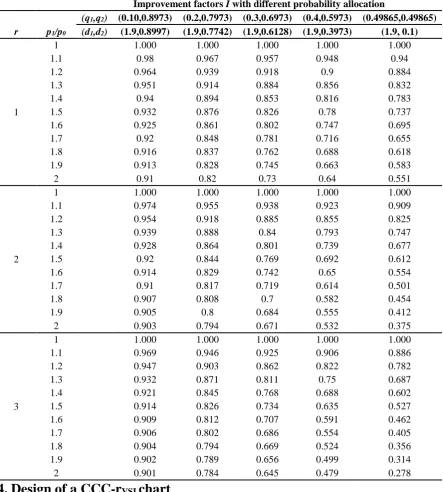
3.5. Improvement factors for different probability allocations

The overall performance of CCCVSI is analyzed based on the equal in-control probability allocations. Thus, in order to investigate the overall performance of CCCVSI chart when the condition q1=q2 = ⋯ =qn is not satisfied, we fix n=2 and d1=1.9 and only change the values

of in control probability q1 as suggested by Liu et al. (2006). It should be noted

that:

1 2

1

q



q

 



. Thus, d2 can

1 1 2

2

1

0 d q d

q



 

  (19)

Thus, q1 should satisfy the inequalityq₁ (1 ) /d₁ for fixed value of d1.

The results in Table 5, indicate that when (q2-q1) decreases, then the improvement factor, I

decreases and the performance of CCC-rVSI charts improves.

Table 5. Improvement factors I with different probability allocation for CCC-r chart with n=2

Improvement factors I with different probability allocation

(q1,q2) (0.10,0.8973) (0.2,0.7973) (0.3,0.6973) (0.4,0.5973) (0.49865,0.49865)

r p1/p0 (d1,d2) (1.9,0.8997) (1.9,0.7742) (1.9,0.6128) (1.9,0.3973) (1.9, 0.1)

1

1 1.000 1.000 1.000 1.000 1.000

1.1 0.98 0.967 0.957 0.948 0.94

1.2 0.964 0.939 0.918 0.9 0.884

1.3 0.951 0.914 0.884 0.856 0.832

1.4 0.94 0.894 0.853 0.816 0.783

1.5 0.932 0.876 0.826 0.78 0.737

1.6 0.925 0.861 0.802 0.747 0.695

1.7 0.92 0.848 0.781 0.716 0.655

1.8 0.916 0.837 0.762 0.688 0.618

1.9 0.913 0.828 0.745 0.663 0.583

2 0.91 0.82 0.73 0.64 0.551

2

1 1.000 1.000 1.000 1.000 1.000

1.1 0.974 0.955 0.938 0.923 0.909

1.2 0.954 0.918 0.885 0.855 0.825

1.3 0.939 0.888 0.84 0.793 0.747

1.4 0.928 0.864 0.801 0.739 0.677

1.5 0.92 0.844 0.769 0.692 0.612

1.6 0.914 0.829 0.742 0.65 0.554

1.7 0.91 0.817 0.719 0.614 0.501

1.8 0.907 0.808 0.7 0.582 0.454

1.9 0.905 0.8 0.684 0.555 0.412

2 0.903 0.794 0.671 0.532 0.375

3

1 1.000 1.000 1.000 1.000 1.000

1.1 0.969 0.946 0.925 0.906 0.886

1.2 0.947 0.903 0.862 0.822 0.782

1.3 0.932 0.871 0.811 0.75 0.687

1.4 0.921 0.845 0.768 0.688 0.602

1.5 0.914 0.826 0.734 0.635 0.527

1.6 0.909 0.812 0.707 0.591 0.462

1.7 0.906 0.802 0.686 0.554 0.405

1.8 0.904 0.794 0.669 0.524 0.356

1.9 0.902 0.789 0.656 0.499 0.314

2 0.901 0.784 0.645 0.479 0.278

4. Design of a CCC-r

VSI

chart

should be determined. According to the methodologies elaborated so for, the design procedure is suggested as follows.

Step 1: Determine the control limits based on fixed false alarm probability.

Step 2: Select the number of sampling intervals.

Step 3: Select the method of probability allocation.

Step 4: Determine the length of sampling intervals (d1, d2,…, dn).

Step 5: Evaluate the efficiency of CCC-rVSI charts: All of the design parameters of the CCC-rVSI chart can be determined by implementing the above four steps. When the shifted nonconforming fraction isp1, then the probability allocation(q q1, 2) can be calculated using

Eq. (16), then the improvement factor I can be computed using Eq. (15), that can be used to evaluate the efficiency of the CCC-rVSI chart.

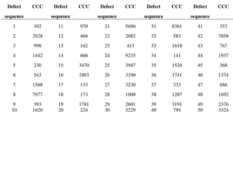
To illustrate the design procedure of a CCCVSI chart, we suppose thatp₀ 0.0005, 0.0027

  , n=2, (d1,d2)=(1.9,0.1). The data of Table 6 show the input defect sequence. As

can be seen in Fig. 1, CCC-rVSI charts are drawn for different values of parameter r. It is concluded that no signal is observed.

Table 6. A set of data follow geometric distribution with nonconforming rate p0= 0.0005

Defect CCC Defect CCC Defect CCC Defect CCC Defect CCC

sequence sequence sequence sequence sequence

1 102 11 970 21 5696 31 8361 41 353

2 2928 12 466 22 2082 32 583 42 7858

3 998 13 162 23 413 33 1618 43 767

4 1442 14 606 24 9235 34 141 44 1937

5 230 15 3470 25 3947 35 1526 45 368

6 543 16 1803 26 3190 36 1741 46 1374

7 1568 17 133 27 3230 37 333 47 686

8 7977 18 173 28 1008 38 1287 48 1692

9 393 19 1781 29 2601 39 3191 49 2376

=2.

n

chart(c) with

VSI

5 -chart(b) and CCC

VSI

2 -chart(a), CCC

VSI

Figure 1. An example of the CCC

0 4000 8000 12000 16000

1 3 5 7 9 11 13 15 17 19 21 23 25 27 29 31 33 35 37 39 41 43 45 47 49

CCC

Defects sequence

CCC

_VSI

chart (a)

CCC LCL IL

UCL

0 8000 16000 24000 32000

1 2 3 4 5 6 7 8 9 10

CCC

Defects Sequence

CCC-5

_VSI

chart (c)

CCC LCL IL1

UCL IL2

0 2000 4000 6000 8000 10000 12000 14000 16000 18000 20000

1 2 3 4 5 6 7 8 9 10 11 12 13 14 15 16 17 18 19 20 21 22 23 24 25

CCC

Defects Sequence

CCC-2

_VSI

chart (b)

CCC

LCL

IL1

5. Conclusion

In this paper, we have proposed the CCC-rVSI control chart for high quality processes. The CCC-r chart is an improved form of CCC charts. Also, we compared CCC-rVSI chart with CCCVSI chart that has been studied by Liu et al. (2006). The results of this study have demonstrated that always CCCVSI chart is more efficient than CCCFSI chart and also CCC-rVSI charts perform better than CCCVSI chart. It is denoted that the efficiency of CCC-rVSI chart can be enhanced by increasing the difference between interval lengths. The results show that when probability allocation is equal, then the performance of CCC-rVSI chart becomes better. In CCC-rVSI chart, if parameter r increases, then the improvement factor of CCC-rVSI chart will decrease. Thus, CCC-rVSI chart can detect the nonconforming fraction shift faster than CCCVSI chart. Also, we compared CCC-rVSI chart with CCC-rFSI chart and concluded that CCC-rVSI chart is always more efficient than CCC-rFSI chart.

References

Amin, R. W., and Miller, R. W., (1993). "A robustness study of X charts with variable sampling intervals", Journal of Quality Technology, Vol. 25, pp. 36-36.

Aparisi, F., and Haro, C. L., (2001). "Hotelling's T2 control chart with variable sampling intervals",

International Journal of Production Research, Vol. 39, No. 14, pp. 3127-3140.

Calvin, T., (1983). "Quality Control Techniques for" Zero Defects", IEEE Transactions on Components, Hybrids, and Manufacturing Technology, Vol. 6, No. 3, pp. 323-328.

Castagliola, P., Celano, G., and Fichera, S., (2006). "Evaluation of the statistical performance of a variable sampling interval R EWMA control chart", Quality Technology & Quantitative Management, Vol. 3, No. 3, pp. 307-323.

Castagliola, P., Celano, G., Fichera, S., and Giuffrida, F., (2006). "A variable sampling interval S2-EWMA control chart for monitoring the process variance", International Journal of Technology Management, Vol. 37, pp. 125-146.

Chen, Y.-K., (2013). "Cumulative conformance count charts with variable sampling intervals for correlated samples", Computers & Industrial Engineering, Vol. 64, No. 1, pp. 302-308.

Chen, Y. K., Chen, C. Y., & Chiou, K. C., (2011). "Cumulative conformance count chart with variable sampling intervals and control limits", Applied stochastic models in business and industry, Vol. 27, No. 4, pp. 410-420.

Epprecht, E. K., Costa, A. F., and Mendes, F. C., (2003). "Adaptive control charts for attributes", IIE Transactions, Vol. 35, No. 6, pp. 567-582.

Goh, T., 1987. A control chart for very high yield processes. Quality Assurance, 13(1), 18-22.

Kudo, K., Ohta, H., and Kusukawa, E., (2004). "Economic Design of A Dynamic CCC–r Chart for High-Yield Processes", Economic Quality Control, Vol. 19, No. 1, pp. 7-21.

Kuralmani, V., Xie, M., Goh, T., and Gan, F., (2002). "A conditional decision procedure for high yield processes", IIE Transactions, Vol. 34, No. 12, pp. 1021-1030.

Lee, M. H., and Khoo, M. B., (2017). "Combined Double Sampling and Variable Sampling Interval np Chart", Communications in Statistics-Theory and Methods (accepted manuscript).

Lee, T.-H., Hong, S.-H., Kwon, H.-M., and Lee, M., (2016). "Economic Statistical Design of Variable Sampling Interval X Control Chart Based on Surrogate Variable Using Genetic Algorithms",

Management and Production Engineering Review, Vol. 7, No. 4, pp. 54-64.

Liu, J., Xie, M., Goh, T., Liu, Q., and Yang, Z., (2006). "Cumulative count of conforming chart with variable sampling intervals", International Journal of Production Economics, Vol. 101, No. 2, pp. 286-297.

Luo, Y., Li, Z., and Wang, Z., (2009). "Adaptive CUSUM control chart with variable sampling intervals", Computational Statistics & Data Analysis, Vol. 53, No. 7, pp. 2693-2701.

Naderkhani, F., and Makis, V., (2016). "Economic design of multivariate Bayesian control chart with two sampling intervals", International Journal of Production Economics, Vol. 174, pp. 29-42.

Noorossana, R., Saghaei, A., Paynabar, K., and Samimi, Y., (2007). "On the conditional decision procedure for high yield processes", Computers & Industrial Engineering, Vol. 53, No. 3, pp. 469-477.

Ohta, H., Kusukawa, E., and Rahim, A., (2001). "A CCC‐r chart for high‐yield processes", Quality and Reliability Engineering International, Vol. 17, No. 6, pp. 439-446.

Reynolds Jr, M. R., and Arnold, J. C., (1989). "Optimal one-sided Shewhart control charts with variable sampling intervals", Sequential Analysis, Vol. 8, No. 1, pp. 51-77.

Reynolds, M. R., Amin, R. W., and Arnold, J. C., (1990). "CUSUM charts with variable sampling intervals", Technometrics, Vol. 32, No. 4, pp. 371-384.

Reynolds, M. R., Amin, R. W., Arnold, J. C., and Nachlas, J. A., (1988). "Charts with variable sampling intervals", Technometrics, Vol. 30, No. 2, pp. 181-192.

Runger, G. C., and Montgomery, D. C., (1993). "Adaptive sampling enhancements for Shewhart control charts", IIE Transactions, Vol. 25, No. 3, pp. 41-51.

Runger, G. C., and Pignatiello Jr, J. J., (1991). "Adaptive sampling for process control", Journal of Quality Technology, Vol. 23, No. 2, pp. 135-155.

Saccucci, M. S., Amin, R. W., and Lucas, J. M., (1992). "Exponentially weighted moving average control schemes with variable sampling intervals", Communications in Statistics-simulation and Computation, Vol. 21, No. 3, pp. 627-657.

Shamma, S. E., Amin, R. W., and Shamma, A. K., (1991). "A double exponentially weighted moving average control procedure with variable sampling intervals", Communications in Statistics-simulation and Computation, Vol. 20, pp. 511-528.

Vaughan, T. S., (1992). "Variable sampling interval np process control chart", Communications in Statistics-Theory and Methods, Vol. 22, No. 1, pp. 147-167.

Villalobos, J. R., Muñoz, L., and Gutierrez, M. A., (2005). "Using fixed and adaptive multivariate SPC charts for online SMD assembly monitoring", International Journal of Production Economics, Vol. 95, No. 1, pp. 109-121.

Xie, M., Goh, T. N., and Kuralmani, V., (2012). "Statistical models and control charts for high-quality processes", Springer Science & Business Media.

Zhang, M., Nie, G., and He, Z., (2014). "Performance of cumulative count of conforming chart of variable sampling intervals with estimated control limits", International Journal of Production Economics, Vol. 150, pp. 114-124.

Zhang, Y., Castagliola, P., Wu, Z., and Khoo, M. B., (2012). "The variable sampling interval X chart with estimated parameters", Quality and Reliability Engineering International, Vol. 28, No. 1, pp. 19-34.