Integrative subspace clustering by common and specific decomposition for applications on cancer subtype identification

R E S E A R C H

Open Access

Integrative subspace clustering by

common and specific decomposition for

applications on cancer subtype identification

Yin Guo, Huiran Li, Menglan Cai and Limin Li

FromJoint 30th International Conference on Genome Informatics (GIW) & Australian Bioinformatics and Computational Biology Society (ABACBS) Annual Conference

Sydney, Australia. 9–11 December 2019

Abstract

Background: Recent high throughput technologies have been applied for collecting heterogeneous biomedical omics datasets. Computational analysis of the multi-omics datasets could potentially reveal deep insights for a given disease. Most existing clustering methods by multi-omics data assume strong consistency among different sources of datasets, and thus may lose efficacy when the consistency is relatively weak. Furthermore, they could not identify the conflicting parts for each view, which might be important in applications such as cancer subtype identification. Methods: In this work, we propose an integrative subspace clustering method (ISC) by common and specific decomposition to identify clustering structures with multi-omics datasets. The main idea of our ISC method is that the original representations for the samples in each view could be reconstructed by the concatenation of a common part and a view-specific part in orthogonal subspaces. The problem can be formulated as a matrix decomposition problem and solved efficiently by our proposed algorithm.

Results: The experiments on simulation and text datasets show that our method outperforms other state-of-art methods. Our method is further evaluated by identifying cancer types using a colorectal dataset. We finally apply our method to cancer subtype identification for five cancers using TCGA datasets, and the survival analysis shows that the subtypes we found are significantly better than other compared methods.

Conclusion: We conclude that our ISC model could not only discover the weak common information across views but also identify the view-specific information.

Keywords: Subtype identification, Multi-view clustering, Subspace clustering

Background

With the advancements of biological technologies, there are many kinds of data available such as genomic DNA copy number arrays, DNA methylation, exome sequenc-ing, messenger RNA arrays, microRNA sequencing and reverse-phase protein arrays and so on. By analyzing the multiple data generated by cancer patients, it is now pos-sible to classify cancer patients to different subgroups, and

*Correspondence:[email protected]

School of Mathematics and Statistics, Xi’an Jiaotong University, Xianning West 28, Xi’an, China

thus improve the diagnostic and treatment. For example, Breast cancer is one of the most common cancers world-wide, and it is clinically categorized into four basic thera-peutic subgroups: (1). Luminal A with oestrogen receptor (ER) positive group; (2). Luminal B with oestrogen recep-tor (ER) positive group; (3) HER2 amplified group; (4) triple-negative breast cancers (TNBCs, also called basal-like, lacking expression of ER, progesterone receptor (PR) and HER2). The ER positive (including Luminal A and B) is the most common and diverse, and several genomic tests can be used to predict outcomes for ER+ patients receiving endocrine therapy. The treatment for the HER2

amplified subtype has a great success due to the effec-tive therapeutic targeting of HER2. The basal-like breast cancers, often with BRCA1 mutations or of African ances-try have only option of chemotherapy. Therefore, subtype identification for breast cancers surely can assist the treat-ment for the patients.

Most molecular studies of subtype identification for breast cancer integrate genomic, epigenomic, and tran-scriptomic profiling including mRNA expression profil-ing, miRNA expression, DNA methylation and DNA copy number analysis, and so on. It is assumed in these stud-ies that integrative clustering of multi-omics data can capture clearer structure that can not be discovered by only exploring a single omic data. In fact, in many other applications, a single object often can be represented by multiple features or views. For example, an image can be represented by its pixels and its captions, an Inter-net webpage can be represented by its text contents and the hyperlinks to other webpages, and a scientific pub-lication can be represented by its text contents and its citations. In all these applications, multi-view clustering takes information from all views into account such that better clustering structures could be discovered.

The difficulty in multi-view learning mainly lies in that the similarity measurement, geometric distribution, clus-tering structure, and noisy levels and so on are often diverse for different views. Samples represented in dif-ferent views may have their own clustering structures, or subspaces they lie in. The differences hamper the cluster-ing significantly. It is challengcluster-ing to efficiently reconcile the conflicting information among views.

Most of existing multi-view clustering approaches fol-low three directions. The first class of methods [1–7] attempt to determine new representations by minimizing the differences or maximizing the correlations between different views. The second class of approaches propagate information from different views to construct graphs or similarities in a slightly different way, including multi-view EM [8], multi-view spectral clustering [9,10], multi-view clustering with unsupervised feature selection [11, 12], nonnegative Matrix Factorization [13], pattern fusion [14], similarity network fusion (SNF) [4]. For example, the similarity network fusion (SNF) [4] fuses multiple net-works to one network by iteratively updating a sequence of nonnegative status matrices. The third class of meth-ods aim to learn an optimal linear combination of multiple kernels or similarities [15–20]. For example, the opti-mized kernel k-means [16] is proposed to obtain opti-mal linear combination of multiple kernels and cluster assignment matrix simultaneously by minimizing a trace clustering loss.

However, almost all the existing methods assume strong consistency among different views or omics, and thus they capture the clustering structure by using the hidden

shared information. This may face problem in the case when the different views share relatively weak common clustering structure. For instance, different views may have different levels of noisy information. Furthermore, different views may have conflicting clustering structures, or one single view may have different clustering structures with all the others. All of these may make it difficult to identify the shared information among views. A biolog-ical example is that, the analysis on different omics for glioblastoma multiforme (GBM), an aggressive adult brain tumor, obtains different results. One work [21] based on expression and copy-number-variant data, identifies two subtypes, which is inconsistent with the results obtained in [22], which identifies four subtypes primarily only by expression data. Therefore, when the consistent informa-tion is weaker than the conflicting informainforma-tion, which is highly likely in subtype identification, it is challenging to discover the hidden clustering structures. A natural idea to overcome this challenge is to decompose the informa-tion in each view to a shared part across all views and a view-specific part. A kernel based method [23] is devel-oped following this idea, which attempts to construct a consensus kernel using multi-omics data. However, for applications, it focuses more on the common part, but ignores the view-specific clustering structure. Further-more, the semi-definite programming for the optimiza-tion problem is computaoptimiza-tional complex.

In this work, we propose a novel integrative subspace clustering method by assuming that the common struc-ture information is weak across views. The main idea is to find a specific subspace for each view, so that the new representation for each sample in each view in this sub-space is a concatenation of two vectors, say, a common representation among all views, and a specific representa-tion for this view. This could make sure that the common parts and the specific parts lie in two orthogonal sub-spaces for each view. Furthermore, the representations of the common part are expected to be independent with those of each specific part, where the dependence is mea-sured by Hilbert Schmidt Independence Criterion (HSIC). Our main contributions in this work are summarized as follows.

1. We propose a novel subspace learning model to discover the common and specific representations for each sample, especially for the case when the

common information might be relatively weaker than the specific information. We propose an algorithm to solve the corresponding optimization problem efficiently.

3. We apply the proposed clustering method on subtype identification, by assuming that the subtype

information may also come from the view-specific part of a single omics data. We apply our approach to identify subtypes for five cancers using TCGA datasets. The survival analysis on the clustering results shows that our method works the best for most cases.

Methods

In this section, we will present the proposed integrative subspace clustering method by multi-view matrix decom-position. We first give a problem statement, and then propose a subspace learning method by mult-view matrix decomposition. We then introduce the Hilbert Schmidt Independence Criterion, and finally propose our integra-tive subspace clustering model ISC and the corresponding optimization algorithm.

Problem statement

Suppose we are given n samples with V views, X =

[X1,· · ·,XV], whereXv ∈ Rpv×n,v = 1,· · ·,V. Denote Xv =[xv1,· · ·,xvn], wherexvi ∈ Rpv. The aim is to cluster thensamples with a given cluster number based on the integrative information from thevviews. In cancer sub-type identification, the views can be different data sources, omics or platforms.

Subspace learning for common and specific decomposition We consider the samples Xv ∈ Rpv×n from view v are approximately lying in a d-dimensional subspacev ⊂

Rpv _{(d < p}

v), which is spanned by the columns of an orthonormal matrixPv ∈ Rpv×d,PTvPv = Id. This means that

xv_i ≈Pvzvi,

wherezv_i ∈Rdis the new representation ofxv_i in this sub-space. We assume that the samplesXv from viewvhave both common and specific clustering structures, which means thatzv_i can be further represented as

zv_i =

ci sv_i

whereci ∈Rd0 is the common representation ofxiacross all views, andsv_i ∈ Rdvis the specific representation ofxi in thev-th view. Note thatd=d0+dv. In other words,xvi can be approximately represented as

xv_i ≈Pvzvi=Pv

ci sv_i

=P(_vc) P_v(s) ci sv_i

=P(_vc)ci+P(vs)svi,

where Pv =

P(vc) Pv(s)

, (P(vc))TP(vc) = Id0 and

Pv(s)

T

P(vs) = Idv. This means that the d-dimensional subspacevspanned byPvis further decomposed to two

orthogonal subspaces(vc)and(vs), spanned by orthonor-mal matricesPv(c) andPv(s), respectively. In other words, v=(c)

v ⊕(vs), wherev(c)and(vs)are orthogonal sub-spaces to each other. We can rewrite the above equations in a matrix form as follows,

Xv = PvZv+Ev

= Pv(c) Pv(s) C Sv

+Ev

= Pv(c)C+Pv(s)Sv+Ev

= Pv

C Sv

+Ev, v=1,· · ·,V

(1)

where Zv =

zv₁,· · ·,zv_n , C = [c1,· · ·,cn], Sv =

sv₁,· · ·,sv_n , andEvis the error matrix for viewv.

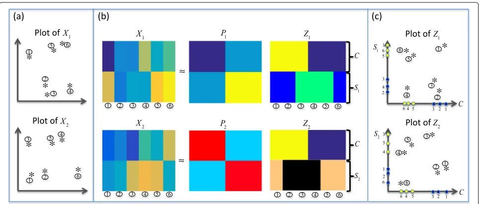
We demonstrate the decomposition idea in Fig.1. We attempt to find two orthogonal subspaces(vc) and(vs) for each viewv, such thatXvcould be decomposed to the common partCand the specific partSv in the subspace v=(c)

v ⊕(vs). Hopefully, the common clustering struc-ture is hidden inC, and the specific clustering structure for viewvis hidden inSv.

Hilbert-Schmidt Independence criterion (HSIC)

To better decompose each view to a common and a view-specific part, such that each view-specific cluster-ing structure inSv is independent to the common part C across all views, a measurement for independence is required. We measure the independence by using the Hilbert-Schmidt Independence Criterion (HSIC) which is a measure of statistical independence [24]. Intuitively, HSIC can be considered as a squared correlation coeffi-cient between two random variablescandscomputed in feature spacesFandG.

Letcandsbe two random variables from the domains C andS, respectively. LetF andG be feature spaces on C andS with associated kernels kc : C× C → Rand ks : S×S →R, respectively. Denote the joint probabil-ity distribution ofcandsbyp₍c,s), and(c,s)and(c,s)are

drawn according top₍c,s). Then the Hilbert Schmidt

Inde-pendence Criterion can be computed in terms of kernel functions via:

HSIC(p₍c,s),F,G)=Ec,c,s,s[kc(c,c)ks(s,s)]

+Ec,c[kc(c,c)] Es,s[ks(s,s)]

−2Ec,s[ Ec[kc(c,c)] Es[ks(s,s)] ] ,

where E is the expectation operator.

The empirical estimator of HSIC for a finite sample of pointsCandSfromcandswithp₍c,s)was given in [24] to

be

Fig. 1Demonstration of the main idea for the common and specific decomposition in our ISC model.ashows the plots forX1andX2respectively.b

shows how the originalXvis decomposed to two partsCandSvin two subspaces.cshows the plots for the reconstructedZv, respectively. Note that the two axes ofZvrepresent two subspaces. We can see that in the two subspaces, the samples are clustered in different ways

wheretris the trace operator of a matrix,His the center-ing matrixH=In−ee

T

n (e is a proper dimensional column vector with all ones), and Kc andKs ∈ Rn×n are kernel matrices. The smaller the HSIC value, the more likelyC

andSare independent from each other.

Integrative subspace clustering (ISC) model

Based on the above considerations, we propose our inte-grative subspace clustering model as follows,

minP1,···,PV C,S1,···,SV

V v=1

Xv−Pv

C Sv 2 F

+βVv=1tr

CTCHST_vSvH

s.t.PT vPv=I,

(3)

whereST_vSv andCTCare the linear kernels ofSvandC, respectively, andβis a parameter. Note that the first term is the decomposition term that tries to find the orthog-onal subspaces where the corresponding common and view-specific representations lie in, and the second inde-pendence term is to minimize the deinde-pendence between the common part and the view-specific part. We use the linear kernel of C and Sv to simplify the computation. AfterCandSvs for all views are obtained,k-means clus-tering is applied to cluster the samples represented byC

and Sv, respectively. The clustering results by using the common partCand the specific partSvare called ISC-C, ISC-S1,ISC-S2,· · ·, respectively.

Based on the resultingCandSis, we define a consensus score(C-score) which is similar to [23] as below:

C-scorei=

trHX_iTXiHCTC

trHX_iTXiH

CT_C+ST i Si

. (4)

C-score is used to measure the weight of the consensus part in thei-th view. Note that the C-score ranges from 0 to 1, and a higher C-score implies stronger consistent information in the corresponding view.

Optimization algorithm

We propose an alternative updating approach to solve the optimization problem (3).

Step 1. We first fixPvandCin (3), and solve for optimal S1,· · ·,Svone by one. Thev-th optimization subproblem can be written as:

min Sv Xv−Pv

C Sv 2 F

+βtr(CTCHST_vSvH). (5)

Since Pv can be represented as Pv = (Pv(c) P(vs)), the subproblem (5) to solve forSvcan be simplified to:

min Sv

tr

−2XvTPv(s)Sv+2STv

P(vs) T

P(vc)C+STv

P(vs) T

P(vs)Sv

+βtrCTCHST_vSvH

(6)

By setting the derivatives of the objective functionf(Sv)in (6) with respect toSvto be zero, we obtain

∂f(Sv) ∂Sv =

0⇒P(_vs)TP_v(s)Sv+βSvHCTCH

=P(_vs)TXv−

P_v(s)TP_v(c)C.

The matrix equation forSvin (7) is a standard Sylvester equation and can be solved efficiently using method in [25].

Step 2. We then fix C,S1,· · ·,SV, and solve the opti-mization problem (3) for optimalP1,· · ·,PV one by one. The correspondingv-th optimization subproblem can be written as:

min

Pv ||Xv−PvZv|| 2

F s.t. PvTPv=I, (8)

where Zv =

C Sv

. The optimization problem (8) is a

least square problem on grassman manifold, and solved by algorithm 2 in [26].

Step 3. We fix P1,· · ·,PV and S1,· · ·,SV, then solve the optimization problem (3) for C. The corresponding subproblem can be written as:

min

C

V

v tr

−2XvTP( c)

v C+2STv

P(vs) T

P(vc)C+CT

Pv(c) T

P(vc)C

+βtrST

vSvHCTCH

.

(9)

Similarly, we set the derivatives of objective function of the subproblem (9) with respect toC, and obtain

_V

v=1

P(_vc)

T P_v(c)

C+βC

_V

v=1

HS_vTSvH

=

V

v=1

P_v(c)TXv−

P(_vc)TP(_vs)Sv.

(10)

The matrix equation for C in (10) is also a standard Sylvester equation and the same algorithm for solving (7) can be used.

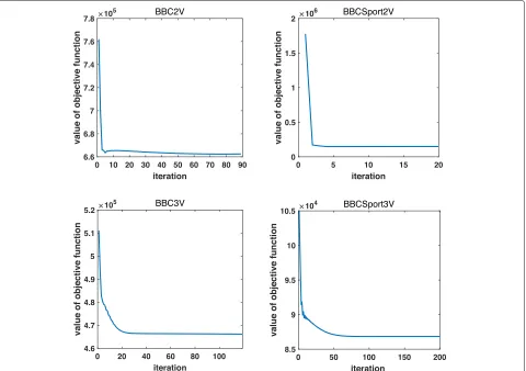
The overall algorithm for solving (3) is shown in the algorithm box ISC. For each iteration, we need to solve three subproblems in our ISC algorithm to alternatively updateSv,Pv andC. Since the objective function of ISC model in (3) has a lower bound of zero. and the objec-tive values of our method is decreasing at each step to solve the three subproblems. Therefore the convergence of objective values in our algorithm can be assured. We also experimentally show the convergence of objective val-ues by using four text datasets in Fig. 2, which further confirms the convergence analysis above.

Results

Comparative methods

We compare our ISC model with the following compara-tive methods.

• Spectral clustering for single views(SV1, SV2).

Algorithm 1Algorithm ISC Input:

Xv∈Rpv×n,v=1,· · ·,V; Output:Pv,Sv,C,v=1,· · ·,V;

1. InitializePv∈Rpv×(d0+dv)by a identical matrix 2. InitializeC∈Rd0×n_randomly

3. while (Pv,Sv,C) not converged 4. for v=1:V

5. Fix the others and updateSvby solving the Eq. (7) 6. Fix the others and updatePvby solving the Eq. (8) 7. end

8. Fix the others and updateCby solving the Eq. (10) 9. end

• Co-regularized spectral clustering (Coreg) [3]. The coreg method extends the single view spectral clustering method by adding a co-regularization term which forces the low embeddings from multiple views to be close.

• Similarity network fusion (SNF) [4]. The SNF method integrates the sample similarity network constructed by each data type into a single similarity network by a nonlinear combination approach. This converged network can be used to cluster multi-view datasets.

• Enhanced consensus multi-view clustering

model(ECMC) [23]. The ECMC method attempts to find the consensus kernels of multiple views by dividing the kernel of each view into a consensus kernel and a disagreement kernel. The method can achieve a relatively good clustering effects even the correlation between views is weak.

Measurements of clustering performance

We use the following three measurements to evaluate the clustering results when the ground truth clustering is given.

• Normalized mutual information (NMI). The

normalized mutual information (NMI) of a clustering resultC= {Ck}is defined as

NMI(C,C∗)= 2MI(C,C ∗₎

H(C)+H(C∗) with

MI(C,C∗)= Ck∈C,C∗∈C∗

pCk,C∗·log2

pCk,C∗

p(C_k)pC∗,

whereC∗= {C∗_l}is the ground truth clustering,

p(Ck):= |Ck|/n,p

Ci,Cj∗

is the joint probability of the two classesCiandC∗j, and

H(C)= −_Ci∈Cp(Ci)log₂(p(Ci)).

Fig. 2Convergence of the objective values of our algorithm on four datasets of BBC2V, BBC3V, BBCSport2V and BBCSport3V

ordering which matches the ground truth labels

l∗_j

ofC∗, the average clustering correction (ACC) is defined as

ACC(C,C∗)= 1

n n

j=1 δlj,lj∗

,

where the functionδ(lj,lj∗)=1iflj=l∗j, or δlj,l∗j

=0otherwise.

• Adjusted rand index (ARI). For a computed clusterCi

and a ground truth clusterC∗_j, letni.= |Ci|, n.j= |C∗j|, andnij= |Ci∩Cj∗|. The adjusted rand

index is defined as

ARI= RI−E(RI) max(RI)−E(RI),

whereRI=_i,jC_nij2 ,

max(RI)= 1_2iC2 ni.+

jC2n.j

, and

E(RI)=_iC_ni2_{. j}C2_n.j/C_n2, whereC represents combination number operator. The range of ARI is from -1 to 1. A larger value of ARI means that the

clustering result is more consistent with the ground truth clustering.

• Silhouette score (S-score) [27]. When the ground truth clustering is unkonwn, the above criterions could not be computed, and thus Silhouette score defined as follows can be used

S-score= 1

n

i

bi−ai max{ai,bi}

,

whereaiis the average Euclidean distance from

samplei to the other samples within the same cluster of samplei andbiis the minimum of the average

Euclidean distance from samplei to all samples in any one of the other clusters different from the cluster of samplei. The range of silhouette score is from -1 to 1. The larger the silhouette score is, the better the clustering structure is.

Simulation experiments

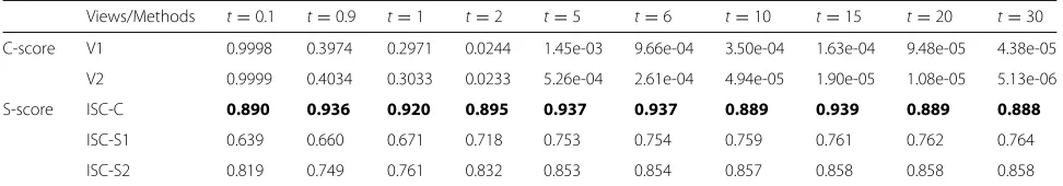
Table 1Consensus scores and Silhouette scores for the simulation datasets

Views/Methods t₌0.1 t₌0.9 t₌1 t₌2 t₌5 t₌6 t₌10 t₌15 t₌20 t₌30

C-score V1 0.9998 0.3974 0.2971 0.0244 1.45e-03 9.66e-04 3.50e-04 1.63e-04 9.48e-05 4.38e-05

V2 0.9999 0.4034 0.3033 0.0233 5.26e-04 2.61e-04 4.94e-05 1.90e-05 1.08e-05 5.13e-06

S-score ISC-C 0.890 0.936 0.920 0.895 0.937 0.937 0.889 0.939 0.889 0.888

ISC-S1 0.639 0.660 0.671 0.718 0.753 0.754 0.759 0.761 0.762 0.764

ISC-S2 0.819 0.749 0.761 0.832 0.853 0.854 0.857 0.858 0.858 0.858

The highest silhouette scores are marked in bold

points evenly from a mixed Gaussian distribution with μ1 =[−4, 6] ,μ2 =[ 3,−10] and a common covariance matrix =[ 10 0; 0 6], and thus could obtain a matrix

Y ∈ R2×200. By adding white noises to Y, we can get two data matricesY1 ∈ R2×200andY2 ∈ R2×200, which can be considered as the common part for two views. We then construct two specific matrices T1 andT2 by ran-domly permuting the columns ofY1andY2, respectively. Finally, we randomly construct two matricesPv ∈ R8×4 and construct the two-view matricesXv = Pv[Yv;tTv]∈

R8×200,(v = 1, 2), where t is a parameter which could control the degree of inconsistency of different views. Note that the ground truth clustering labels for both com-mon part, and the two specific parts are both known and denoted byy,y1,y2. We construct 10 corresponding datasets by takingt= {0.1, 0.9, 1, 2, 5, 6, 10, 15, 20, 30}. We report the consensus scores for two views on simulation datasets in Table1. From the table, we can see that simula-tion datasets with smallthave high consensus scores and those with largethave low consensus scores.

Table 2The average NMIs, ACCs and ARIs obtained by the our ISC method and other comparison partners in simulation datasets

Methods t=0.1 t=0.9 t=1 t=2 t=5 t=6 t=10 t=15 t=20 t=30

NMI SV1 0.368 0.012 0.003 0.005 0.019 0.020 0.024 0.023 0.023 0.023

SV2 1.000 0.009 0.006 0.001 0.004 0.005 0.006 0.006 0.006 0.006

Coreg 0.701 0.072 0.039 0.005 0.007 0.006 0.010 0.012 0.010 0.012

SNF 1.000 1.000 1.000 0.960 0.592 0.161 0.000 0.000 0.000 0.000

ECMC 1.000 0.203 0.051 0.006 0.016 0.020 0.019 0.024 0.023 0.023

ISC-C 1.000 1.000 1.000 1.000 1.000 1.000 1.000 1.000 1.000 1.000

ISC-S1 0.004 0.301 0.390 0.673 0.806 0.806 0.759 0.759 0.736 0.736

ISC-S2 0.005 0.756 0.816 0.862 0.889 0.889 0.889 0.889 0.889 0.889

ACC SV1 0.840 0.563 0.530 0.540 0.580 0.582 0.590 0.590 0.590 0.590

SV2 1.000 0.555 0.545 0.515 0.535 0.540 0.545 0.545 0.545 0.545

Coreg 0.945 0.655 0.615 0.540 0.550 0.545 0.558 0.565 0.560 0.565

SNF 1.000 1.000 1.000 0.995 0.900 0.730 0.505 0.505 0.505 0.505

ECMC 1.000 0.663 0.599 0.535 0.575 0.582 0.579 0.588 0.586 0.587

ISC-C 1.000 1.000 1.000 1.000 1.000 1.000 1.000 1.000 1.000 1.000

ISC-S1 0.537 0.810 0.850 0.940 0.970 0.970 0.960 0.960 0.955 0.955

ISC-S2 0.540 0.955 0.970 0.980 0.985 0.985 0.985 0.985 0.985 0.985

ARI

SV1 0.460 0.011 -0.001 0.001 0.021 0.022 0.028 0.028 0.028 0.028

SV2 1.000 0.007 0.003 -0.004 -0.000 0.001 0.003 0.003 0.003 0.003

Coreg 0.791 0.092 0.048 0.001 0.005 0.003 0.009 0.012 0.009 0.012

SNF 1.000 1.000 1.000 0.980 0.638 0.208 -0.004 -0.004 -0.004 -0.004

ECMC 1.000 0.229 0.063 0.003 0.018 0.022 0.021 0.028 0.027 0.027

ISC-C 1.000 1.000 1.000 1.000 1.000 1.000 1.000 1.000 1.000 1.000

ISC-S1 0.001 0.381 0.487 0.773 0.883 0.883 0.846 0.846 0.827 0.827

ISC-S2 0.001 0.827 0.883 0.921 0.941 0.941 0.941 0.941 0.941 0.941

We first compare the three clustering results obtained by our method and show their performance when t

changes. We apply our ISC model to compute the corre-sponding common part Cand the specific partsS1and S2. k-means clustering is then applied on C, S1 andS2, and three corresponding clustering results ISC-C, ISC-S1 and ISC-S2 are obtained, respectively. Since thek-means method may be sensitive to the initials, we run the k -means method 100 times and report the average of the results. We choose the parameterβfrom{0, 1e−6, 1e−

5,· · ·, 1e+5, 1e+6}. We report the average Silhouette scores for the three clustering results in Table1. As we can see, the clustering result of ISC-C achieves a higher silhou-ette score than the clustering results of ISC-S1 and ISC-S2 for anyt, which indicates that the common part may have better clustering structure in the simulation datasets. We also compute the NMI, ACC and ARI by comparing the

three clustering results with the ground truth labelsy,y1 and y2, respectively. The average values are reported in Table2. We have two observations from the results. First, ISC-C peforms perfect when t changes, and the results by ISC-S1 and ISC-S2 are getting better whentincreases. This means that the our ISC-C could always capture the common structure even the consisitency is very weak, and our ISC-S1 and ISC-S2 could capture the specific structures better when the consistency gets weak. Second, ISC-C achieves higher NMI, ACC and ARI values than ISC-S1 and ISC-S2, which is consistent with the results obtained by silhouette scores. This implies that Silhouette scores may be used to select the best clustering result.

We then compare our clustering result by ISC-C with the comparison methods by computing NMI, ACC, and ARI of each methods, which all assume strong consis-tency across views except ECMC. The average values of

all the methods are reported in Table2. Whentis rela-tively small, almost all the methods could perform well. When the degree of inconsistency increases astincreases, our method ISC-C outperforms other methods. That is because, when the consistency signal is very weak, existing methods could not capture the common clustering struc-ture any more, but our ISC-C could discover the common clustering structure very well. We also plot the clustering results for all multi-view methods witht=0.1 andt=10 in Fig.3. In the figure, since the common result of the SNF method is in the form of the kernel, we present all the data in the form of a kernel. Specifically, as for the simulation datasets, the linear kernel ofXv,YvandTvare denoted as Kv,KvcandKvs, respectively. In addition, when using a lin-ear kernel, equationsKv =Kvc+Kvshold forv= 1, 2. We can see that in Fig.3a,tis small and consensus score is big, and all methods could discover the latent common clus-tering structure with high accuracy. However, in Fig.3b, when t is big and the consensus score is low, all base-line methods fail to discover the best clustering structure, but our ISC-C method could still capture the common structure across views. This further shows the power of our method even when the common information is very weak.

Experiments on multi-view text datasets

In this section, we evaluate our ISC method on multi-view text datasets. Since only the ground truth labels for com-mon part is known, we compare the ISC-C results with other methods.

• BBC and BBCSport datasets. BBC datasets consist of 2,225 documents provided by the BBC News website, which are stories about the five thematic areas of business, entertainment, politics, sports and technology from 2004 to 2005. The BBCSport datasets consist of 737 documents from the BBC Sports website, which correspond to sports news articles in the five subject areas of sports, cricket, football, rugby and tennis from 2004 to 2005. Each article is divided into up to four parts, each part has at least 200 characters, and then the pieces are randomly assigned to each view, which can generate the dataset of BBC2/3/4views and BBCSport2/3/4views. Here we only select BBC2/3views, BBCSport2/3views datasets for clustering.

• Cora dataset. The Cora dataset consists of machine learning papers that are one of seven categories: case-based, genetic algorithms, neural networks,

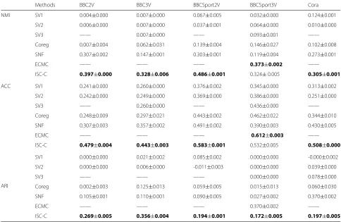
Table 3The average NMIs, ACCs, ARIs and standard errors obtained by the ISC and other comparison partners on text datasets

Methods BBC2V BBC3V BBCSport2V BBCSport3V Cora

NMI SV1 0.004±0.000 0.007±0.000 0.067±0.005 0.032±0.000 0.124±0.001

SV2 0.006_±0.000 0.007_±0.000 0.037_±0.001 0.064_±0.000 0.010_±0.000

SV3 —— 0.007_±0.000 —— 0.093_±0.001 ——

Coreg 0.007_±0.004 0.062_±0.031 0.139_±0.004 0.146_±0.027 0.102_±0.008

SNF 0.307±0.002 0.147±0.001 0.303±0.001 0.119±0.004 0.273±0.001

ECMC —— —— —— 0.373±0.002 ——

ISC-C 0.397±0.000 0.328±0.006 0.486±0.001 0.324±0.005 0.305±0.001

ACC SV1 0.241_±0.000 0.260_±0.000 0.376_±0.002 0.345_±0.000 0.313_±0.002

SV2 0.242_±0.000 0.249_±0.000 0.369_±0.000 0.386_±0.000 0.251_±0.000

SV3 —— 0.260_±0.000 —— 0.436_±0.000 ——

Coreg 0.248_±0.009 0.297_±0.021 0.443_±0.002 0.462_±0.022 0.344_±0.010

SNF 0.307±0.003 0.357±0.002 0.491±0.002 0.390±0.003 0.430±0.005

ECMC —— —— —— 0.612±0.003 ——

ISC-C 0.479±0.004 0.443±0.003 0.583±0.001 0.532±0.005 0.508±0.000

ARI

SV1 0.000_±0.000 0.021_±0.002 0.085_±0.002 0.000_±0.000 -0.000_±0.002

SV2 0.000_±0.000 0.006_±0.000 -0.011_±0.003 0.000_±0.000 0.039_±0.000

SV3 —— —— —— 0.000_±0.000 0.078_±0.000

Coreg 0.002±0.003 0.125±0.013 0.059±0.005 0.015±0.013 0.060±0.030

SNF 0.105±0.001 0.110±0.001 0.090±0.005 0.027±0.002 0.370±0.002

ECMC —— —— —— 0.370±0.002 ——

ISC-C 0.269±0.005 0.356±0.004 0.194±0.001 0.172±0.005 0.197±0.005

probabilistic methods, reinforcement learning, rule learning, and theory. There are 2,708 papers in the entire corpus. The dataset consists of two views. One view is represented by a 0/1 value word vector, indicating the absence/presence of the corresponding word in the dictionary. The other view is the citation relationship between each publication and other publications.

By using the ISC model, we could obtain the common partC. We then apply k-means clustering onC. We com-pare the results of ISC-C with other methods, and the results are shown in Table3. We can see from the table that, our ISC model works the best for most cases.

Identifying cancer types by colorectal cancer dataset Tumors may not be diagnosed pathologically, and thus it’s meaningful to determine whether the patient’s spe-cific symptoms are colon cancer or colorectal cancer. We further evaluate our method by identifying colon cancer and colorectal cancer on a colorectal cancer

dataset [28]. which consists exome sequences, DNA copy number, promoter methylation and messenger RNA, and microRNA expression for 276 patients. We select three types of expression data including DNA methylation, mRNA expression and miRNA expression. Specifically, DNA methylation profiles are obtained by the Illumina Infinium HumanMethylation27 arrays, mRNA expression profiles are generated by Agilent microarray, and miRNA quantification via Illumina sequencing. After screening, we obtain 85 cancer patients with colon cancer and col-orectal cancer.

We apply our ISC model to identify the cancer types (colon cancer or colorectal caner) for these patients with two or three views, and obtain the corresponding com-mon partCand three specific partsS1,S2 andS3. Since we assume that the cancer type or subtype structures may be specifically shown in a single omics, we check the clus-tering results for both the common and specific parts and see whether they capture the clustering information for cancer types. Note that the ground truth for cancer types is known, thus we could also calculate NMI, ACC

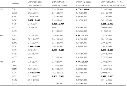
Table 4The average NMIs, ACCs and ARIs and standard errors obtained by the ISC and other comparison partners on colorectal cancer datasets

Methods DNA methylation+ DNA methylation+ miRNA expression+ DNA methylation+miRNA

miRNA expression mRNA expression mRNA expression expression+mRNA expression

NMI SNF 0.247±0.001 0.247±0.004 0.330±0.003 0.276±0.000

Coreg 0.023_±0.000 0.186_±0.000 0.186_±0.000 0.234_±0.008

ECMC 0.164_±0.000 0.164_±0.000 0.091_±0.004 0.138_±0.006

ISC-C 0.372_±0.006 0.149_±0.001 0.137_±0.015 0.012_±0.004

ISC-S1 0.118±0.005 0.338±0.004 —— 0.288±0.002

ISC-S2 0.019±0.002 —— 0.046±0.007 0.009±0.005

ISC-S3 —— 0.175±0.002 0.263±0.003 0.178±0.001

ACC SNF 0.835_±0.004 0.800_±0.006 0.847_±0.003 0.835_±0.005

Coreg 0.812_±0.000 0.812_±0.000 0.812_±0.000 0.812_±0.000

ECMC 0.741_±0.000 0.741_±0.000 0.642_±0.005 0.706_±0.004

ISC-C 0.871_±0.003 0.602_±0.002 0.689_±0.000 0.567_±0.004

ISC-S1 0.698±0.004 0.859±0.004 —— 0.843±0.006

ISC-S2 0.583±0.009 —— 0.685±0.008 0.566±0.002

ISC-S3 —— 0.779±0.007 0.828±0.001 0.757±0.003

ARI SNF 0.391_±0.003 0.310_±0.005 0.442_±0.004 0.402_±0.004

Coreg 0.031_±0.003 0.250_±0.000 0.250_±0.000 0.336_±0.013

ECMC 0.209_±0.000 0.209_±0.000 0.080_±0.005 0.160_±0.006

ISC-C 0.506±0.001 -0.007±0.009 0.113±0.003 0.000±0.017

ISC-S1 0.139±0.000 0.469±0.006 —— 0.422±0.005

ISC-S2 0.015±0.002 —— 0.098±0.008 0.011±0.009

ISC-S3 —— 0.238±0.005 0.384±0.006 0.237±0.006

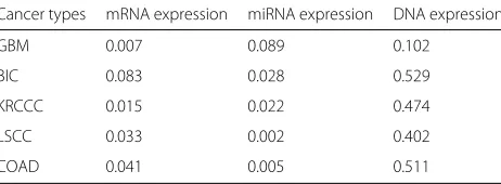
Table 5Consensus scores of three views for the five TCGA cancer datasets

Cancer types mRNA expression miRNA expression DNA expression

GBM 0.007 0.089 0.102

BIC 0.083 0.028 0.529

KRCCC 0.015 0.022 0.474

LSCC 0.033 0.002 0.402

COAD 0.041 0.005 0.511

and ARI by using the common part ISC-C, the specific parts ISC-S1, ISC-S2, ISC-S3. The results are reported in Table4. Our method performs better than the base-line methods for most of the cases. Overall, our method ISC-C with common part with DNA methylation and miRNA expression data performs the best among all the obtained clustering results. While for miRNA and mRNA expression, SNF works the best, our ISC method with the specific part of DNA methylation (ISC-S1) works the best among all methods on the view combinations with DNA methylation. It may imply that DNA methylation plays an important role in the identification of the cancer type. This confirms our hypothesis that information about the type of cancer may be hidden in a particular omics.

Applications on cancer subtype identification using TCGA datasets

We finally apply our ISC model on The Cancer Genome Atlas (TCGA) Research Network[29] to identify subtypes for five cancers. TCGA is currently the largest database of cancer genetic information, and has included 33 types of cancer including 10 rare cancer types. In addition, in the database, each cancer data contains gene expression data, miRNA expression data, copy number variation, DNA methylation, SNP, etc., and has sufficient clinical data.

Data sets

The datasets for five cancers using TCGA datasets are collected by Wang et al. [4]. The datasets contain five cancer types: polymorphism Glioblastoma (GBM), renal clear cell carcinoma (KRCCC), breast invasive carcinoma (BIC), colon adenocarcinoma (COAD) and lung squa-mous cell carcinoma (LSCC). There are three types of cancer expression data: DNA methylation, mRNA expres-sion, and miRNA expresexpres-sion, as well as clinical infor-mation, including survival data for patients. Since we don’t have the ground truth labels for the subtypes of these datasets, survival analysis is mainly used to evaluate our model.

For each of the five datasets, we apply the ISC model to compute the common part and specific parts, and then apply k-means to obtain clustering results. The procedure for obtaining the cancer subtype of the dataset is the same as that of Colorectal cancer dataset. The numbers of sub-types are chosen as 3, 3, 4, 3 and 4 for GBM, KRCCC, BIC, COAD, and LACC[4], respectively. We also report consensus scores for the three views of the five cancers in Table5. As we can see, the consensus scores for the first two views are both very low. This implies that the consistency information across views are relatively weaker compared to the inconsistency, and thus the traditional multi-view methods may not work.

Survival analysis

We apply the log-rank test to measure whether different subtypes obtained by clustering are meaningful, since the survival time in months are given for each sample in the TCGA datasets . The log-rank test is a commonly used non-parametric test method for comparison of survival processes in survival analysis and can be used to compare whether two or more sets of survival curves are identical. In general, the smaller thep-value obtained from it, the

Table 6Coxp-values of survival analysis obtained by different clustering methods for the five cancers in TCGA datasets

Methods GBM BIC KRCCC LSCC COAD

mRNA expression 5.67e-01 9.30e-02 9.54e-01 6.00e-03 1.93e-01

DNA Methylation 1.55e-01 5.77e-04 8.11e-01 1.30e-02 1.10e-02

miRNA expression 1.88e-01 9.80e-01 8.34e-01 1.17e-01 7.14e-01

Coreg 2.00e-03 4.81e-05 1.63e-04 5.00e-03 7.00e-03

SNF 8.00e-03 3.46e-05 8.00e-03 1.66e-04 2.00e-03

ECMC 1.70e-02 7.26e-06 1.00e-02 6.95e-04 3.87e-04

ISC-C 3.66e-08 2.62e-04 1.04e-04 9.19e-12 2.11e-02

ISC-S1 4.00e-03 1.44e-03 2.56e-04 8.07e-06 7.68e-03

ISC-S2 8.05e-05 6.12e-05 2.55e-04 2.67e-13 7.12e-04

ISC-S3 3.00e-03 3.28e-06 1.92e-04 2.45e-04 3.20e-02

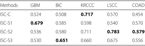
Table 7Silhouette scores by different clustering methods for the five cancers in TCGA datasets

Methods GBM BIC KRCCC LSCC COAD

ISC-C 0.524 0.508 0.717 0.570 0.454

ISC-S1 0.679 0.585 0.598 0.540 0.570

ISC-S2 0.536 0.580 0.711 0.783 0.579

ISC-S3 0.530 0.651 0.660 0.675 0.556

The highest silhouette scores are marked in bold

more different the survival curves of the two or more groups.

The log-rankp-values for all the methods are reported in Table6. we can see from the table that, for four can-cers including GBM, BIC, KRCCC, and LSCC, our ISC method could obtain the most significant p-values. For COAD, our method with ISC-S2 could obtain the simi-larly goodp-value with the ECMC method. Furthermore, the subtypes for GBM and KRCCC found by the common

part across three views obtain the most significant p -values, the BIC subtypes found by miRNA expression are the most significant, and the subtypes for LSCC found by DNA methylation are the most significant. We also report the silhouette scores for the clustering results of ISC-C, ISC-S1, ISC-S2, and ISC-S3 in Table7. By comparing Tables 6 and 7, for four of five datasets except GBM, the best clustering results with the best cox p-values among our four clustering results are corresponding to the highest silhouette scores. This implies that the our selec-tion sheme for the clustering results is effective in this application.

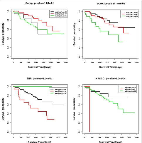
We also plot the Kaplan-Meier survival curves by the ISC clustering results with the most significantp-values for all the five cancer types. Figure4shows the curves for GBM, BIC, COAD, and LSCC, and Fig.5shows the curve for KRCCC. From the figures, we could see the signifi-cantly different survival profiles over the subtypes. For the cancer KRCCC, we also plot the Kaplan-Meier survival curves obtained by baseline methods Coreg, ECMC and

Fig. 5Kaplan-Meier survival curves for KRCCC by four methods: Coreg, ECMC, SNF and ISC (p-values are reported in Table6)

SNF in Fig.5. We can see the survival curves by our ISC method are more significantly different than that obtained by the other compared methods.

Subtype visualization

We further analyze the obtained breast cancer subtypes by our model ISC withS3, sinceS3 by miRNA expression generates the most significantly different survival profiles across different subtypes. Fig.6 shows the visualization

Fig. 6Visualization of the three data types in four subtypes for Breast cancer

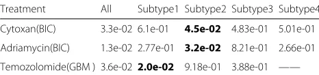
Drug treatment analysis on cancer subtypes

We finally validate the obtained subtypes by compar-ing the survival profiles from different treatment groups in each subtype. We choose two drug treatments of Cytoxan and Adriamycin for breast cancer, and drug treatment temozolomide for GBM. For each subtype, we check whether the survival profiles are significantly dif-ferent between the treatment patients and the untreated patients. The Cox p-values for all the three treatments in all subtypes are reported in Table 8. Interestingly, we can see that for breast cancer, the patients in Subtype 2 is sensitive to the two drug treatments of Cytoxan and Adri-amycin. The Kaplan-Meier survival curves of these two

Table 8Survival analysis of three treatments on four BIC subtypes and three GBM subtypes

Treatment All Subtype1 Subtype2 Subtype3 Subtype4

Cytoxan(BIC) 3.3e-02 6.1e-01 4.5e-02 4.83e-01 5.01e-01 Adriamycin(BIC) 1.3e-02 2.77e-01 3.2e-02 8.21e-01 2.66e-01 Temozolomide(GBM ) 3.6e-02 2.0e-02 9.18e-01 3.88e-01 —— The treatment can significantly improve treatment outcomes in the subtype of p-value in boldface

treatments in Subtype 2 are shown in Fig.7. In Subtype 1 of GBM, the patients with treatment temozolomide have significantly different survival profiles with the untreated patients in this subtype. the Kaplan-Meier survival curves of glio cancers in Subtype 1 is shown in Fig. 8. These further validate that the Subtypes we cound is biological meaningful.

Discussion on breast subtypes

We further discuss the subtypes we found for breast cancer. Breast cancer is a heterogeneous and polygenic disease, which is one of the most common malignancies in women. Based on histological and genomic features, breast cancer can be roughly separated into four sub-types (luminal A, luminal B, HER2-amplified, and basal-like) [30].

Fig. 7Survival analysis of the treatment with Cytoxan and Adriamycin in Breast cancer Subtype 2 withp-values 4.45e-02 and 3.23e-02, respectively

of deletion event in the basal cancers, which is related with basal-like cancer enriched subgroup, harbours chro-mosome 5q deletions, and several signaling molecules, transcription factors and cell division genes [31]. Besides, basal-like subtype may also correlate with the gene EGFR, which is supported with the fact that alterations of EGFR, p53 and pTeN are cooperative and likely to play an impor-tant role in basal-like breast cancer pathogenesis[32]. For luminal B subtype, PPP2R2A is an associated gene due to the dysregulation of specific PPP2R2A functions in

Fig. 8Survival analysis of the Temozolomide treatment in GBM subtype 1 withp-value 2e-2

luminal B breast cancers [31]. The genes ZNF703 and DHRS2 are likely to correlate with luminal B since [33] suggests ZNF703 is a luminal B specific driver and Tumors with elevated ZNF703 levels were characterized by alter-ations in a lipid metabolism and detoxification pathway that include DHRS2 as a key signaling component. For HER2 subtype, [34] confirms that agents targeting GAB2 or GAB2-dependent pathways may be useful for treating breast tumors that overexpress HER2, and thus we include GAB2 as a correlated gene for HER2 type breast cancer. Besides, Trastuzumab blocks the HER2-HER3(ERBB3) interaction and is used to treat breast cancers with HER2 overexpression, although some of these cancers develop trastuzumab resistance. By using small interfering RNA (siRNA) to identify genes involved in trastuzumab resistance, [35] identified several kinases and phos-phatases that were upregulated in trastuzumab-resistant cancers, including PPM1H. This suggests that PPM1H and ERBB3 may have some link with HER2 type breast cancer.

For each computed subtype by our ISC algorithm, we first calculate t-testp-values for each of these correlated

Table 9Groupp-values for three breast cancer subtypes including basal-like, luminal B and HER2

Groupp-values Subtype1 Subtype2 Subtype3 Subtype4

Basal-like 1.69e-01 3.83e-08 1.50e-02 4.79e-07

Luminal B 2.44e-01 3.91e-02 1.17e-02 3.03e-02

HER2 1.09e-01 3.34e-01 5.69e-03 4.17e-07

genes to show whether the gene expression levels are sig-nificantly changed between the subtype and the other subtypes. We then apply the Fisher’s combined proba-bility test [36] to compute the group p-values for these genes, which could test whether the group of the selected genes are significantly different between the subtype the and other subtypes. We report the group p-values for each resulting subtype in Table9. The results show that, our computed Subtype 2 is highly likely corresponding to the basal-like breast cancer subtype, with group p-value being 3.83e-08. Our computed Subtype 4 may also contain the basal-like breast cancer subtype, with group p-value being 4.79e-07. Our Subtype 4 probably corresponds to the HER2 breast cancer subtype, with groupp-value being 4.17e-07, and our Subtype 3 is likely to correspond to the luminal B breast cancer subtype.

Conclusion

Our goal in this work is to discover common and spe-cific information simultaneously from multi-views when the consistency across views is relatively weak, and the specific signal is strong. We propose integrative subspace clustering method (ISC) by common and specific decom-position to find two orthogonal subspaces for each view. To better distinguish the common and view-specific part, we also hope the common part and view-specific part are as independent as possible by using the measurement HSIC. Our simulation experiments, real-world bench-mark experiments, cancer type identification by colorectal data, subtype identification for five cancers by TCGA datasets all show that the ISC model outperforms other state-of-art multi-view clustering algorithms. In particu-lar, we find some interesting subtypes in breast cancer and GBM cancer, and the survival analysis shows that the subtypes are biologically meaningful.

Abbreviations

BIC: Breast cancer; COAD: Colon cancer; GBM: Glio cancer; HSIC: Hilbert Schmidt Independence Criterion; ISC-C: Clustering by the common part in our ISC method; ISC-S: Clustering by the specific part in our ISC method; KRCCC: Kidney cancer; LSCC: Lung cancer; SV: Single view; TCGA: The cancer genome atlas

Acknowledgements

Supported by the NSFC projects 11631012, Shanghai Municipal Science and Technology Major Project (No.2018SHZDZX01), LCNBI and ZJLab, and the Fundamental Research Funds for the Central Universities.

About this supplement

This article has been published as part ofBMC Medical Genomics Volume 12 Supplement 9, 2019: Proceedings of the Joint International GIW & ABACBS-2019 Conference: medical genomics. The full contents of the supplement are available online athttps://bmcmedgenomics.biomedcentral.com/articles/ supplements/volume-12-supplement-9.

Authors’ contributions

YG designed the optimization algorithms and conducted the experiments. HL conducted the survival analysis. LL and MC designed the model and the experiments, and wrote the manuscript. All authors revised and approved the manuscript.

Funding

The publication charges for this article were funded by the Fundamental Research Funds for the Central Universities.

Availability of data and materials

Multi-view text datasetswere downloaded fromhttp://mlg.ucd.ie/ datasets/bbc.html.Colorectal cancer datasetwas downloaded fromhttp:// www.cbioportal.org/study/summary?id=coadread_tcga_pub.TCGA datasetswere downloaded on 18/4/2017 fromhttp://compbio.cs.toronto. edu/SNF/SNF/Software.html.

Ethics approval and consent to participate

Not applicable.

Consent for publication

Not applicable.

Competing interests

The authors declare that they have no competing interests.

Received: 11 November 2019 Accepted: 19 November 2019 Published: 24 December 2019

References

1. Tang W, Lu Z, Dhillon I. Clustering with multiple graphs. 2009;24(4): 1016–21.https://doi.org/10.1109/icdm.2009.125.

2. Chaudhuri K, Kakade S, Livescu K, Sridharan K. Multi-view clustering via canonical correlation analysis. In: International Conference on Machine Learning; 2009. p. 129–36.https://doi.org/10.1145/1553374.1553391. 3. Kumar A, Rai P, Daumé H. Co-regularized multi-view spectral clustering.

In: Advances in Neural Information Processing Systems 24: 25th Annual Conference on Neural Information Processing Systems 2011. Proceedings of a Meeting Held. Granada; 2012. p. 1413–14.http://papers.nips.cc/ paper/4360-coregularized-multi-view-spectral-clustering.

4. Wang B, Mezlini A, Demir F, Fiume M, Tu Z, Brudno M, Haibekains B, Goldenberg A. Similarity network fusion for aggregating data types on a genomic scale. Nat Methods. 2014;11(3):333.

5. Blum A, Mitchell T. Combining labeled and unlabeled data with co-training. In: Proceedings of the Eleventh Annual Conference on Computational Learning Theory; 1998. p. 92–100.https://doi.org/10. 1145/279943.279962.

6. Muslea I, Minton S, Knoblock C. Active learning with multiple views. J Artif Intell Res. 2006;27:203–33.

7. Wang.W, Zhou.Z. A new analysis of co-training. In: Proceedings of the 27th International Conference on Machine Learning (ICML-10); 2010. p. 1135–1142.

8. Bickel S, Scheffer T. Multi-view clustering. In: ICDM; 2004. p. 19–26.

https://doi.org/10.1109/icdm.2004.10095.

9. Kumar A, III HD. A co-training approach for multiview spectral clustering. In: Proceedings of the 28thInternational Conference on Machine Learning, ICML. Bellevue; 2011. p. 393–400.https://icml.cc/2011/papers/ 272icmlpaper.pdf.

10. Xia R, Pan Y, Du L, Yin J. Robust multi-view spectral clu stering via low-rank and sparse decomposition. In: Proceedings of the Twenty-Eighth AAAI Conference on Artificial Intelligence. Québec; 2014. p. 2149–55. 11. Tang J, Hu X, Gao H, Liu H. Unsupervised feature selection for multi-view

data in social media. In: SDM; 2013. p. 270–8.https://doi.org/10.1137/1. 9781611972832.30.

12. Wang H, Nie F, Huang H. Multi-view clustering via joint nonnegative matrix factorization. In: Proceedings of the 13th SIAM International Conference on Data Mining. Austin; 2013. p. 352–60.http://proceedings. mlr.press/v28/wang13c.html.

13. Gao J, Han j, Liu j, Wang c. Multi-view clustering via joint nonnegative matrix factorization. In: Proceedings of the 13th SIAM International Conference on Data Mining. Austin; 2013. p. 252–60.https://doi.org/10. 1137/1.9781611972832.28.

14. Qianqian S, Chuanchao Z, Minrui P, Xiangtian Y, Tao Z, Juan L, Luonan C. Pattern fusion analysis by adaptive alignment of multiple

15. Lanckriet G, Cristianini N, Bartlett P, El G, Jordan M. Learning the kernel matrix with semi-definite programming. J Mach Learn Res. 2002;5(1): 27–72.

16. Yu S, Tranchevent L, Liu X, Glanzel W. Optimized data fusion for kernel k-means clustering. Pattern Anal Mach Intell IEEE Trans. 2011;34(5):1031–9. 17. Lange T, Buhmann J. Fusion of similarity data in clustering. In: Advances

in Neural Information Processing Systems 18. Vancouver: NIPS; 2005. p. 723–30. http://papers.nips.cc/paper/2880-fusion-of-similarity-data-in-clustering.

18. Chuang Y. Affinity aggregation for spectral clustering. IEEE Conf Comput Vis Pattern Recogn. 2012;23(10):773–80.

19. Gönen M, Margolin A. Localized data fusion for kernel k-means clustering with application to cancer biology. Adv Neural Inf Process Syst. 2014;2: 1305–13.

20. Bach F, Lanckriet G, Jordan M. Multiple kernel learning, conic duality, and the smo algorithm. In: International Conference; 2004. p. 6.https://doi. org/10.1145/1015330.1015424.

21. Nigro JM, Misra A, Zhang L, Smirnov I, Colman H, Griffin C, Ozburn N, Chen M, Pan E, Koul D, Yung WKA, Feuerstein BG, Aldape KD. Integrated array-comparative genomic hybridization and expression array profiles identify clinically relevant molecular subtypes of glioblastoma. Cancer Res. 2005;65(5):1678–86.

22. Verhaak Roel GW, et al. Integrated genomic analysis identifies clinically relevant subtypes of glioblastoma characterized by abnormalities in pdgfra, idh1, egfr, and nf1. Cancer Cell. 2010;17(1):98–110.

23. Cai M, Li L. Subtype identification from heterogeneous tcga datasets on a genomic scale by multi-view clustering with enhanced consensus. BMC Med Genomics. 2017;4:75:.https://doi.org/10.1186/s12920-017-0306-x. 24. Gretton A, Bousquet O, Smola A J, Schölkopf B. Measuring statistical

dependence with hilbert-schmidt norms. In: ALT; 2005. p. 63–77.https:// doi.org/10.1007/11564089_7.

25. Bartels RH, Stewart GW. Solution of the matrix equation ax+xb=c [f4] (algorithm 432). Commun Acm. 1972;15(9):820–6.

26. Wen, Zaiwen. A feasible method for optimization with orthogonality constraints. Math Program. 2013;142(1-2):397–434.

27. Rousseeuw PJ. Silhouettes: A graphical aid to the interpretation and validation of cluster analysis. J Comput Appl Math. 1999;20(20):53–65. 28. Network CGA, et al. Comprehensive molecular characterization of human

colon and rectal cancer. Nature. 2012;487(7407):330.

29. Network TCGA. The cancer genome atlas. 2006.http://cancergenome.nih. gov/. Accessed 20 Jun 2019.

30. Parker JS, Mullins M, Cheang MC, et al. Supervised risk predictor of breast cancer based on intrinsic subtypes. J Clin Oncol. 2009;27(8):1160–7. 31. Curtis C, Shah SP, Chin SF, Turashvili G, Rueda OM, Dunning MJ, Speed

D, Lynch AG, Samarajiwa S, Yuan Y. The genomic and transcriptomic architecture of 2,000 breast tumours reveals novel subgroups. Nature. 2012;486(7403):346–52.

32. Pires MM, Hopkins BD, Saal LH, Parsons RE. Alterations of egfr, p53 and pten that mimic changes found in basal-like breast cancer promote transformation of human mammary epithelial cells. Cancer Biol Ther. 2013;14(3):246–53.

33. Holland DG, Burleigh A, Git A, Goldgraben MA, Perezmancera PA, Chin SF, Hurtado A, Bruna A, Ali HR, Greenwood W. Znf703 is a common luminal b breast cancer oncogene that differentially regulates luminal and basal progenitors in human mammary epithelium. Embo Mol Med. 2015;3(3):167–80.

34. Bentires-Alj M, Gil SG, Chan R, Wang ZC, Wang Y, Imanaka N, Harris LN, Richardson A, Neel BG, Gu H. A role for the scaffolding adapter gab2 in breast cancer. Nat Med. 2006;12(1):114.

35. Leehoeflich S, Pham T, Dowbenko D, Munroe X, Lee J, Li L, Zhou W, Haverty P, Pujara K, Stinson J. Ppm1h is a p27 phosphatase implicated in trastuzumab resistance. Cancer Discov. 2011;1(4):326–37.

36. Fisher R, Vol. 118. Statistical Methods for Research Workers; 1954, pp. 66–70.https://doi.org/10.2307/2528855.

Publisher’s Note