T
IME
4: Time for SDN
Technical Report
†, February 2016
Tal Mizrahi, Yoram Moses
∗Technion — Israel Institute of Technology
Email:
{
dew@tx, moses@ee
}
.technion.ac.il
Abstract—With the rise of Software Defined Networks (SDN), there is growing interest in dynamic and centralized traffic engineering, where decisions about forwarding paths are taken dynamically from a network-wide perspective. Frequent path re-configuration can significantly improve the network performance, but should be handled with care, so as to minimize disruptions that may occur during network updates.
In this paper we introduce TIME4, an approach that uses accurate time to coordinate network updates.TIME4is a powerful tool in softwarized environments, that can be used for various network update scenarios. Specifically, we characterize a set of update scenarios calledflow swaps, for whichTIME4is the optimal update approach, yielding less packet loss than existing update approaches. We define the lossless flow allocation problem, and formally show that in environments with frequent path allocation, scenarios that require simultaneous changes at multiple network devices are inevitable.
We present the design, implementation, and evaluation of a TIME4-enabled OpenFlow prototype. The prototype is publicly available as open source. Our work includes an extension to the OpenFlow protocol that has been adopted by the Open Networking Foundation (ONF), and is now included in OpenFlow 1.5. Our experimental results show the significant advantages of TIME4 compared to other network update approaches, and demonstrate an SDN use case that is infeasible without TIME4.
Time is what keeps everything from happening at once
– Ray Cummings
I. INTRODUCTION
A. It’s About Time
The use of synchronized clocks was first introduced in the 19th century by the Great Western Railway company in
Great Britain. Clock synchronization has significantly evolved since then, and is now a mature technology that is being used by various different applications, from mobile backhaul networks [3] to distributed databases [4].
The Precision Time Protocol (PTP), defined in the IEEE 1588 standard [5], can synchronize clocks to a very high degree of accuracy, typically on the order of 1 microsecond [3], [6], [7]. PTP is a common and affordable feature in commodity switches. Notably, 9 out of the 13 SDN-capable switch sili-cons listed in the Open Networking Foundation (ONF) SDN Product Directory [8] have native IEEE 1588 support [9]–[17].
†This report is an extended version of [1], which was accepted to IEEE INFO-COM ’16, San Francisco, April 2016. A preliminary version of this report was published in arXiv [2] in May, 2015.
∗Yoram Moses is the Israel Pollak academic chair at Technion.
In this work we introduce TIME4, a generictool for using time in SDN. One of the products of this work is a new feature that enables timed updates in OpenFlow, and has been incorporated in OpenFlow 1.5. Furthermore, we present a class of update scenarios in which the use of accurate time is provably optimal, while existing update methods are sub-optimal.
B. The Challenge of Dynamic Traffic Engineering in SDN
Defining network routes dynamically, based on a complete view of the network, can significantly improve the network performance compared to the use of distributed routing pro-tocols. SDN and OpenFlow [18], [19] have been leading trends in this context, but several other ongoing efforts offer similar concepts. The Interface to the Routing System (I2RS) working group [20], and the Forwarding and Control Element Separation (ForCES) working group [21] are two examples of such ongoing efforts in the Internet Engineering Task Force (IETF).
Centralized network updates, whether they are related to network topology, security policy, or other configuration at-tributes, often involve multiple network devices. Hence, up-dates must be performed in a way that strives to minimize temporary anomalies such as traffic loops, congestion, or disruptions, which may occur during transient states where the network has been partially updated.
While SDN was originally considered in the context of campus networks [18] and data centers [22], it is now also being considered for Wide Area Networks (WANs) [23], [24], carrier networks, and mobile backhaul networks [25].
WAN and carrier-grade networks require a very low packet loss rate. Carrier-grade performance is often associated with the term five nines, representing an availability of 99.999%. Mobile backhaul networks require a Frame Loss Ratio (FLR) of no more than 10−4 for voice and video traffic, and no more than 10−3 for lower priority traffic [26]. Other types of carrier network applications, such as storage and financial trading require even lower loss rates [27], on the order of 10−5.
Several recent works have explored the realm of dynamic path reconfiguration, with frequent updates on the order of minutes [23], [24], [28], enabled by SDN. Interestingly, for voice and video traffic, a frame loss ratio of up to10−4implies that service must not be disrupted for more than6milliseconds per minute. Hence, if path updates occur on a per-minute basis,
then transient disruptions must be limited to a short period of no more than a few milliseconds.
C. Timed Network Updates
We explore the use ofaccurate timeas a tool for performing coordinated network updates in a way that minimizes packet loss. Softwarized management can significantly benefit from using time for coordinating network-wide orchestration, and for enforcing a given order of events. We introduce TIME4, which is an update approach that performs multiple changes at different switches at the same time.
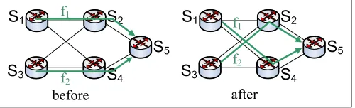
Example 1. Fig. 1 illustrates aflow swappingscenario. In this
scenario, the forwarding paths of two flows,f1andf2, need to
be reconfigured, as illustrated in the figure. It is assumed that all links in the network have an identical capacity of 1 unit, and that bothf1and f2 require a bandwidth of 1 unit. In the
presence of accurate clocks, by schedulingS1andS3to update
their paths at the same time, there is no congestion during the update procedure, and the reconfiguration is smooth. As clocks will typically be reasonably well synchronized, albeit not perfectly synchronized, such a scheme will result in a very short period of congestion.
S1
S2
S
3S4
S
5f1
f2
S1
S2
S
3S
4S5
f1f2
before after
Fig. 1: Flow Swapping—Flows need to convert from the “before” configuration to the “after”.
In this paper we show that in a dynamic environment, where flows are frequently added, removed or rerouted, flow swaps are inevitable. A notable example of the importance of flow swaps is a recently published work by Fox Networks [29], in which accurately timed flow swaps are essential in the context of video switching.
One of our key results is that simultaneous updates are the optimal approach in scenarios such as Example 1, whereas other update approaches may yield considerable packet loss, or incur higher resource overhead. Note that such packet loss can be reduced either by increasing the capacity of the communication links, or by increasing the buffer memories in the switches. We show that for a given amount of resources, TIME4 yields lower packet loss than other approaches.
Accuracy is a key requirement in TIME4; since updates
cannot be applied at the exact same instant at all switches, they are performed within a short time interval called the
scheduling error. The experiments we present in Section IV show that the scheduling error in softwareswitches is on the order of 1 millisecond. The TCAM-based hardwaresolution of [30] can execute scheduled events in existing switches with an accuracy on the order of 1 microsecond.
Accurate time is a powerful abstraction for SDN program-mers, not only for flow swaps, but also fortimed consistent
updates, as discussed by [31].
D. Related Work
Time and synchronized clocks have been used in various distributed applications, from mobile backhaul networks [3] to distributed databases [4]. Time-of-day routing [32] routes traffic to different destinations based on the time-of-day. Path calendaring [33] can be used to configure network paths based on scheduled or foreseen traffic changes. The two latter examples are typically performed at a low rate and do not place demanding requirements on accuracy.
Various network update approaches have been analyzed in the literature. A common approach is to use a sequence of configuration commands [28], [34]–[36], whereby theorderof execution guarantees that no anomalies are caused in interme-diate states of the procedure. However, as observed by [28], in some update scenarios, known asdeadlocks, there is no order that guarantees a consistent transition.Two-phaseupdates [37] use configuration version tags to guarantee consistency during updates. However, as per [37], two-phase updates cannot guarantee congestion freedom, and are therefore not effective in flow swap scenarios, such as Fig. 1. Hence, in flow swap scenarios the order approach and the two-phase approach produce the same result as the simple-minded approach, in which the controller sends the update commands as close as possible to instantaneously, and hopes for the best.
In this paper we present TIME4, an update approach that is most effective in flow swaps and other deadlock [28] scenarios, such as Fig. 1. We refer to update approaches that do not use time asuntimed update approaches.
In SWAN [23], the authors suggest that reserving un-used scratch capacity of 10-30% on every link can allow congestion-free updates in most scenarios. The B4 [24] ap-proach prevents packet loss during path updates by temporarily reducing the bandwidth of some or all of the flows. Our ap-proach does not require scratch capacity, and does not reduce the bandwidth of flows during network updates. Furthermore, in this paper we show that variants of SWAN and B4 that make use of TIME4 can perform better than the original versions.
A recently published work by Fox Networks [29] shows that accurately timed path updates are essential for video swapping. We analyze this use case further in Section IV.
Rearrangeably non-blocking topologies (e.g., [38]) allow new traffic flows to be added to the network by rearranging existing flows. The analysis of flow swaps presented in this paper emphasizes the requirement to perform simultaneous
reroutes during the rearrangement procedure, an aspect which has not been previously studied.
application in which timed updates are the optimal update approach.
E. Contributions
The main contributions of this paper are as follows:
• We consider a class of network update scenarios called
flow swaps, and show that simultaneous updates using synchronized clocks are provably the optimal approach of implementing them. In contrast, existing approaches for consistent updates (e.g., [28], [37]) are not applicable to flow swaps, and other update approaches such as SWAN [23] and B4 [24] can perform flow swaps, but at the expense of increased resource overhead.
• We use game-theoretic analysis to show that flow swaps are inevitable in the dynamic nature of SDN.
• We present the design, implementation and evaluation of a prototype that performs timed updates in OpenFlow. • Our work includes an extension to the OpenFlow protocol
that has been approved by the ONF and integrated into OpenFlow 1.5 [41], and into the OpenFlow 1.3.x exten-sion package [42]. The source code of our prototype is publicly available [43].
• We present experimental results that demonstrate the ad-vantage of timed updates over existing approaches. More-over, we show that existing update approaches (SWAN and B4) can be improved by using accurate time. • Our experiments include an emulation of an
SDN-controlled video swapping scenario, a real-life use case that has been shown [29] to be infeasible with previous versions of OpenFlow, which did not include our time extension.
II. THELOSSLESSFLOWALLOCATION(LFA) PROBLEM
A. Inevitable Flow Swaps
Fig. 1 presents a scenario in which it is necessary toswap
two flows, i.e., to update two switches at the same time. In this section we discuss the inevitability of flow swaps; we show that there does not exist a controller routing strategy that avoids the need for flow swaps.
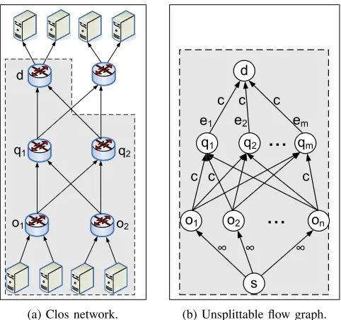
Our analysis is based on representing the flow-swap problem as an instance of an unsplittable flow problem, as illustrated in Fig. 2b. The topology of the graph in Fig. 2b models the traffic behavior to a given destination in common multi-rooted network topologies such as fat-tree and Clos (Fig. 2a).
The unsplittable flow problem [44] has been thoroughly discussed in the literature; given a directed graph, a source node s, a destination node d, and a set of flow demands (commodities) between sand d, the goal is to maximize the traffic rate from the source to the destination. In this paper we define agame between two players: a source1 that generates
traffic flows (commodities) and acontrollerthat reconfigures the network forwarding rules in a way that allows the network to forward all traffic generated by the source without packet losses.
1The source player does not represent a malicious attacker; it is an
‘adversary’, representing the worst-case scenario.
d
q1 q2
o1 o2
(a) Clos network.
d
o1 o2 on
q1 q2 qm
c c c
s ∞
∞ ∞
c c c
e1 e2 em
(b) Unsplittable flow graph.
Fig. 2: Modeling a Clos topology as an unsplittable flow graph.
Our main argument, phrased in Theorem 1, is that the source has a strategy thatforcesthe controller to perform a flow swap, i.e., to reconfigure the path of two or more flows at the same time. Thus, a scenario in which multiple flows must be updated at the same time is inevitable, implying the importance of timed updates.
Moreover, we show that the controller can be forced to invoken individual commands that should optimally be per-formed at the same time. Update approaches that do not use time, also known asuntimedapproaches, cause the updates to be performed over a long period of time, potentially resulting in slow and possibly erratic response times and significant packet loss. Timed coordination allows us to perform the
n updates within a short time interval that depends on the scheduling error.
Although our analysis focuses on the topology of Fig.2b, it can be shown that the results are applicable to other topologies as well, where the source can force the controller to perform a swap over the edges of the min-cut of the graph.
B. Model and Definitions
We now introduce thelossless flow allocation (LFA) prob-lem; it is not presented as an optimization problem, but rather as a game between two players: asourceand acontroller. As the source adds or removes flows (commodities), the controller reconfigures the forwarding rules so as to guarantee that all flows are forwarded without packet loss.The controller’s goal is to find a forwarding path for all the flows in the system without exceeding the capacity of any of the edges, i.e., to completely avoid loss of packets from the given flows. The
source’s goalis to progressively add flows, without exceeding
Our model makes three basic assumptions: (i) each flow has a fixed bandwidth, (ii) the controller strives to avoid
packet loss, and (iii) flows areunsplittable. We discuss these
assumptions further in Sec. V.
The term flow in classic flow problems typically refers to the amount of traffic that is forwarded through each edge of the graph. Since our analysis focuses on SDN, we slightly divert from the common flow problem terminology, and use the term flow in its OpenFlow sense, i.e., a set of packets that share common properties, such as source and destination network addresses. A flow in our context, can be seen as a session between the source and destination that runs traffic at a fixed rate.
The network is represented by a directed weighted acyclic graph (Fig. 2b), G= (V, E, c), with a sources, a destination
d, and a set of intermediate nodes, Vin. Thus, V = Vin∪
{s, d}. The nodes directly connected tosare denoted byO=
{o1, o2, . . . , on}. Each of the outgoing edges from the source
s has an infinite capacity, whereas the rest of the edges have a capacity c. For the sake of simplicity, and without loss of generality, throughout this section we assume thatc= 1. Such a graph Gis referred to as anLFA graph.
The source node progressively transmits traffic flows to-wards the destination node. Each flow represents a session between s and d; every flow has a constant bandwidth, and cannot be split between two paths. A centralized controller configures the forwarding policy of the intermediate nodes, determining the path of each flow. Given a set of flows froms
tod, the controller’s goal is to configure the forwarding policy of the nodes in a way that allows all flows to be forwarded todwithout exceeding the capacity of any of the edges.
The set of flows that are generated bysis denoted byF::=
{F1, F2, . . . , Fk}. Each flowFi is defined asFi::= (i, fi, ri),
whereiis a unique flow index,fi is the bandwidth satisfying
0 < fi ≤ c, and ri denotes the node that the controller
forwards the flow to, i.e.,ri∈ {o1, o2, . . . , on}.
It is assumed that the controller monitors the network, and thus it is aware of the flow set F. The controller maintains a
forwarding function, Rcon : F×Vin −→ Vin∪ {d}. Every
node (switch) has a flow table, consisting of a set of entries; an element w∈F×Vin is referred to as anentryfor short.
An update of Rcon is defined to be a partial function u : F×Vin*Vin∪ {d}. We define arerouteas an updateuthat
has a single entry in its domain. We call an update that has more than one entry in its domain a swap, and it is assumed that all updates in aswapare performed at the same time. We define ak-swap fork≥2as a swap that updates entries in at least kdifferent nodes. Note that ak-swap is possible only if
n≥k, where n is the number of nodes in O. We focus our
analysis on 2-swaps, and throughout the section we assume that n≥2. In Section II-F we discussk-swaps for values of
k >2.
C. The LFA Game
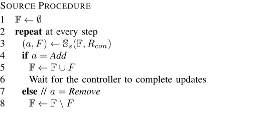
The lossless flow allocation problem can be viewed as a game between two players, the source and the controller. The game proceeds by a sequence of steps; in each step the source
either adds or removes a single flow (Fig. 3), and then waits for the controller to perform a sequence of updates (Fig. 4). The source’s strategySs(F, Rcon) = (a, F), is a function that
defines for each flow setFand forwarding functionRconfor F, a pair (a, F) representing the source’s next step, where
a ∈ {Add,Remove} is the action to be taken by the source, andF = (j, fj, rj) is a single flow to be added or removed.
The controller’s strategy is defined byScon(Rcon, a, F) =U,
whereU={u1, . . . , u`} is a sequence of updates, such that
(i) at the end of each update no edge exceeds its capacity, and (ii) at the end of the last update, u`, the forwarding function
Rcon defines a forwarding path for all flows inF. Notice that
when a flow is to be removed, the controller’s update is trivial; it simply removes all the relevant entries from the domain of
Rcon. Hence our analysis focuses onaddingnew flows.
The following theorem, which is the crux of this section, argues that the source has a strategy that forces the controller to perform a swap, and thus that flow swaps are inevitable from the controller’s perspective.
Theorem 1. LetG be an LFA graph. In the LFA game over
G, there exists a strategy,Ss, for the source that forces every controller strategy,Scon, to perform a2-swap.
Proof: Let m be the number of incoming edges to the destination nodedin the LFA graph (see Fig 2b). Form= 1 the claim is trivial. Hence, we start by proving the claim for m = 2, i.e., there are two edges connected to node d, edgese1 ande2. We show that the source has a strategy that, regardless of the controller’s strategy, forces the controller to use a swap. In the first four steps of the game, the source generates four flows, F1 = (1,0.35, o1), F2 = (2,0.35, o1), F3 = (3,0.45, o2), and F4 = (4,0.45, o2), respectively. According to the Source Procedure of Fig. 3, after each flow is added, the source waits for the controller to update Rcon
before adding the next flow. After the flows are added, there are two possible cases:
(a) The controller routes symmetrically through e1 and e2, i.e. a flow of0.35and a flow of0.45through each of the edges. In this case the source’s strategy at this point is to generate a new flowF5 = (5,0.3, o1)with a bandwidth of0.3. The only way the controller can accommodateF5 is by routingF1andF2through the same edge, allowing the new0.3flow to be forwarded through that edge. Since there is no sequence of reroute updates that allows the
SOURCEPROCEDURE
1 F← ∅
2 repeat at every step
3 (a, F)←Ss(F, Rcon)
4 ifa=Add
5 F←F∪F
6 Wait for the controller to complete updates 7 else// a=Remove
8 F←F\F
CONTROLLERPROCEDURE
1 repeatat every step
2 {u1, . . . , u`} ←Scon(Rcon, a, F)
3 forj∈[1, `]
4 UpdateRconaccording touj
Fig. 4: The LFA game: the controller’s procedure.
controller to reach the desiredRcon, the only way to reach
a state whereF1andF2are routed through the same edge is to swap a0.35flow with a0.45flow. Thus, by issuing
F5 the controller forces a flow swap as claimed. (b) The controller routesF1andF2through one edge, andF3
andF4 through the other edge. In this case the source’s strategy is to generate two flows, F6 and F7, with a bandwidth of 0.2 each. The controller must route F6 through the edge withF1andF2. Now each path sustains a bandwidth of0.9units. Thus, whenF7is added by the source, the controller is forced to perform a swap between one of the0.35flows and one of the0.45flows. In both cases the controller is forced to perform a 2-swap, swapping a flow fromo1 with a flow fromo2. This proves the claim for m= 2.
The case ofm >2is obtained by reduction to m= 2: the source first generatesm−2flows with a bandwidth of1each, causing the controller to saturate m−2 edges connected to node d (without loss of generalitye3, . . . , em). At this point
there are only two available edges,e1ande2. From this point, the proof is identical to the case ofm= 2.
The proof of Theorem 1 showed that the controller can be forced to perform a flow swap that involvesm= 2paths. For
m > 2, we assumed that the source saturates m−2 paths,
reducing the analysis to the case of m= 2. In the following theorem we show that form >2the controller can be forced to perform bm
2cswaps.
Theorem 2. Let Gbe an LFA graph. In the LFA game over
G, if m >2 then there exists a strategy, Ss, for the source
that forces every controller strategy, Scon, to perform bm2c 2-swaps.
Proof: Assume that m is even. The source generates m
flows with a bandwidth of 0.35, m flows with a bandwidth of 0.45, andmflows with a bandwidth of0.2. The only way the controller can route these flows without packet loss is as follows: each path sustains three flows with three different bandwidths,0.2,0.35, and 0.45. Now the source removes the
mflows of0.2, and adds m2 flows of0.3. As in case (a) of the proof of Theorem 1, adding each flow of0.3causes a2-swap. The controller is thus is forced to perform m2 =bm
2cswaps. If mis odd, then the source can saturate one of the edges by generating a flow with a bandwidth of 1, and then repeat the procedure above for the remainingm−1 edges, yielding
m−1
2 =b
m
2cswaps.
For simplicity, throughout the rest of this section we assume that m= 2. However, as in Theorem 2, the analysis can be extended to the case ofm >2.
D. The Impact of Flow Swaps
We define a metric for flow swaps, by considering the oversubscription that is caused if the flows are notswapped simultaneously, but updated using an untimed approach.
We define theoversubscriptionof an edge,e, with respect to a forwarding function,Rcon, to be the difference between the
total bandwidth of the flows forwarded througheaccording to
Rcon, and the capacity ofe. If the total bandwidth of the flows
through e is less than the capacity ofe, the oversubscription is defined to be zero.
Definition 1 (Flow swap impact). Let F be a flow set, and
Rcon be the corresponding forwarding function. Consider a
2-swap u:F×V*V∪ {d}, such thatu=u1∪u2, where ui= (wi, vi), forwi∈F×V,vi ∈V∪ {d}, andi∈ {1,2}. The impact of u is defined to be the minimum of: (i) The oversubscription caused by applying u1 to Rcon, or (ii) the
oversubscription caused by applyingu2 toRcon.
Example 2. We observe the scenario described in the proof of
Theorem 1, and consider what would happen if the two flows had not been swapped simultaneously. The scenario had two cases; in the first case, the bandwidth through each edge is0.8
before the controller swaps a0.35flow with a0.45flow. Thus, if the 0.35 flow is rerouted and then the 0.45 flow, the total bandwidth through the congested edge is 0.8 + 0.35 = 1.15, creating a temporary oversubscription of0.15. Thus, the flow swap impact in the first case is0.15. In the second case, one edge sustains a bandwidth of0.7, and the other a bandwidth of
0.9. The controller needs to swap a0.35flow with a0.45flow. If the controller first reroutes the 0.45 flow, then during the intermediate transition period, the congested edge sustains a bandwidth of0.7 + 0.45 = 1.15, and thus it is oversubscribed by0.15. Hence, the impact in the second case is also0.15.
The following theorem shows that in the LFA game, the source can force the controller to perform a flow swap with a swap impact of roughly0.5.
Theorem 3. Let G be an LFA graph, and let 0 < α <0.5.
In the LFA game over G, there exists a strategy, Ss, for the source that forces every controller strategy, Scon, to perform a swap with an impact of α.
Proof:Let= 0.1−0.2·α. We use the source’s strategy from the proof of Theorem 1, with the exception that the band-widthsf1, . . . , f7of flowsF1, . . . , F7are:f1=f2= 0.5−2, f3=f4= 0.5−,f5= 4, andf6=f7= 3.
the controller is forced to swap between F1 and F3. We compute the impact by considering an untimed update, where the controller reroutesF3first, causing an oversubscription of 1−4+ 0.5−−1 = 0.5−5=α. In both cases the source inflicts a flow swap with an impact of α.
Intuitively, Theorem 3 shows that not only are flow swaps inevitable, but they have a high impact on the network, as they can cause links to be congested by roughly50%beyond their capacity.
E. Network Utilization
Theorem 1 demonstrates that regardless of the controller’s policy, flow swaps cannot be prevented. However, the proof of Theorem 1 uses a scenario in which the edges leading to node dare almost fully utilized, suggesting that perhaps flow swaps are inevitable only when the traffic bandwidth is nearly equal to the max-flow of the graph. Arguably, as suggested in [23], by reserving some scratch capacityν·cthrough each of the edges, for 0< ν <1, it may be possible to avoid flow swaps. In the next theorem we show that if ν < 13, then flow swaps are inevitable.
Theorem 4. Let G be an LFA graph, in which a scratch
capacity ofν is reserved on each of the edgese1, . . . , em, and
letν < 13. In the LFA game overG, there exists a strategy for
the source, Ss, that forces every controller strategy, Scon, to perform a swap.
Proof: We consider a graphG0, in which the capacity of each of the edgese1, . . . , emis1−ν. By Theorem 3, for every
0< α <0.5, there exists a strategy for the source that forces
a flow swap with an impact ofα. Thus, there exists a strategy that forces at least one of the edges to sustain a bandwidth of
α·(1−ν). Sinceν < 13, we have(1−ν)>23, and thus there exists an α <0.5such thatα·(1−ν)>1. It follows that in the original graph G, with scratch capacity ν, there exists a strategy for the source that forces the controller to perform a flow swap in order to avoid the oversubscribed bandwidth of
α·(1−ν)>1.
The analysis of [23] showed that a scratch capacity of 10% is enough to address the reconfiguration scenarios that were considered in that work. Theorem 4 shows that even a scratch capacity of 3313% does not suffice to prevent flow swaps scenarios. It follows that the 10% reserve that [23] suggest may not be sufficient in general for lossless reconfiguration.
F. n-Swaps
As defined above, a k-swap is a swap that involves k or more nodes. In previous subsections we discussed 2-swaps. The following theorem generalizes Theorem 1 to n-swaps, wherenis the number of nodes in O.
Theorem 5. Let Gbe an LFA graph. In the LFA game over
G, there exists a strategy,Ss, for the source that forces every controller strategy,Scon, to perform ann-swap.
Proof: For n = 1, the claim is trivial. For n = 2, the claim was proven in Theorem 1. Thus, we assume n≥3.
Ifm >2, the source first generatesm−2flows with a ratec
each, and we assume without loss of generality that after the controller allocates these flows onlye1ande2remain unused. Thus, we focus on the case wherem= 2.
We describe a strategy, Ss as required; s generates three
types of flows:
• Type A: two flows F1, F2, at a rate of h each: F1 =
(1, h, o1), andF2= (2, h, o1).
• Type B: n flows,F3, . . . , Fn+2, with a total rate g, i.e., at a rate of gn each. The source sends each of thenflows through a different node ofO.
• Type C:n−1flows,Fn+3, . . . , F2n+1with a total rateg, i.e., n−g1 each. The source sends each of then−1 flows through a different node ofo2, . . . , on.
We definehandg such that:
1
3 < h < g <
1
2 (1)
g >(n2−n)(1−2h) (2)
We claim that for everynthere existgandhthat satisfy (1) and (2). We prove this claim by findinggandhthat satisfy the two conditions. We choose an arbitrarygin the range(1124,12). We find a validhby solvingg >(n2−n)(1−2h). The latter yieldsh > 12− α
2(n2−n). Sincen≥3, we haven
2−n≥6, and
thus 2(n2g−n) <
0.5
2×6 =
1
24. Clearly,
g
2(n2−n) >0. It follows
that every hthat satisfies 12− 1
24 < h <
1
2−0, also satisfies
h > 1
3. Hence, everyg andhin the range( 11
24,
1
2)that satisfy
h < g, also satisfy (1) and (2).
Intuitively, forhandgsufficiently close to 12 (but less than 1
2) (1) and (2) are satisfied.
We now prove that after generating the flowsF1, . . . , F2n+1, the functionRconforwards all type B flows through the same
path, and all type C flows through the same path. Assume by way of contradiction that there is a forwarding functionRcon
that forwards flowsF1, . . . , F2n+1 without loss, but does not comply to the latter claim. We consider two distinct cases: either the two type A flows are forwarded through the same edge, or they are forwarded through two different edges.
• If the two type A flows are forwarded through two different paths, then we assume that F1 and the n type B flows are forwarded through e1 and that F2 and the n−1 type C flows are forwarded through e2. Thus, at this point each of the two edges sustains traffic at a rate of g+h. By the assumption, there exists an update that swaps i < n flows of type B with j < n−1 flows of type C, such that after the swap none of the edges exceeds its capacity. Thus, the update adds the bandwidth |j·n−g1−i·ng| to one of the edges, and this additional bandwidth must fit into the available bandwidth before the update,1−g−h. Hence,|j·n−g1−i·gn|< c−g−h. Note that 1−g−h < 1−2h < n−g1 −ng, following (1) and (2). Thus we get|j·ng−1−i·ng|<n−g1−ng. It follows that|j·n−i·n+i|<1. Sincej, i, nare integers, we get thatj·n−i·n+i= 0, and thusj=i·n−1
n . Now
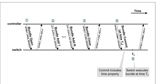
switch
Time controller
Ts B
u n d le C o m m it (a
t tim e T
s)
Switch executes
bundle at time Ts
B u n d le O
p e n
B u n d le A
d d 1
...
Commit may include
scheduled time Ts
1
rep ly
B u n d le A
d d N
B u n d le C
lo s
e re
ply
re ply
2 3 4
B u n d le D
isc a rd 5'
5
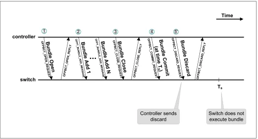
Fig. 5: AScheduled Bundle: theBundle Commitmessage may includeTs, the scheduled time of execution. The controller
can use aBundle Discard message to cancel the Scheduled Bundlebefore timeTs.
the only solution is j =n−1 andi=n, which means that the flows from type B are all forwarded through the same path, as well as the flows of type C, contradicting the assumption.
• If the two type A flows are forwarded through the same edge, their total bandwidth is2h, and thus the remaining bandwidth through this edge is1−2h. From (2) we have
g n−1−
g
n >1−2h. We note that (i) g n−1 >
g n−1−
g n, and
(ii) ng > n−g1−g
n. It follows that g
n−1 >1−2h, and also
g
n >1−2h, and thus none of the type B or type C flows
fit on the same path with F1 andF2. Thus, all the type B and type C flows are on the same path, contradicting the assumption.
We have shown that all flows of type B, denoted by FB,
must be forwarded through the same path, and that all flows of type C, denoted by FC, are forwarded through the same
path. Thus, after the source generates the2·n+ 1flows, there are two possible scenarios:
• The two type A flows are forwarded through the same path, and the type B and type C flows are forwarded through the other path. In this casesgenerates two flows at a rate of1−h−g each. To accommodate both flows the controller must swap the flows of FB with F1 or the flows of FC with F2. Both possible swaps involve n entries, and thus the controller is force to perform an
n-swap.
• One path is used forF1and the flows ofFC, and the other
path is used for F2 and the flows ofFB. In this case the
source generates a flow with a bandwidth of1−2h, again forcing the controller to swap the flows of FB with F1 or the flows of FC withF2.
In both cases the controller is forced to perform a swap that involves the nnodes, i.e., ann-swap.
III. DESIGN ANDIMPLEMENTATION
A. Protocol Design
1) Overview
A TIME4-enabled system is comprised of two main com-ponents:
• OpenFlow time extension. TIME4 is built upon the
OpenFlow protocol. We define an extension to the Open-Flow protocol that enables timed updates; the controller
can attach an execution time to every OpenFlow com-mand it sends to a switch, defining when the switch should perform the required command. It should be noted that the TIME4 approach is not limited to OpenFlow; we have defined a similar time extension to the NETCONF protocol [45], but in this paper we focus on TIME4 in the context of OpenFlow, as described in the next subsection.
• Clock synchronization. TIME4 requires the switches
and controller to maintain a local clock, allowing time-triggered events. Hence, the local clocks should be syn-chronized. The OpenFlow time extension we defined does not mandate a specific synchronization method. Various mechanisms may be used, e.g., the Network Time Protocol (NTP), the Precision Time Protocol (PTP) [5], or GPS-based synchronization. The prototype we designed and implemented uses REVERSEPTP [46], as described below.
2) OpenFlow Time Extension
We present an extension that allows OpenFlow controllers to signal the time of execution of a command to the switches. This extension is described in full in Appendix A.2
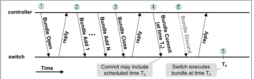
Our extension makes use of the OpenFlow [19] Bundle feature; a Bundle is a sequence of OpenFlow messages from the controller that is applied as a single operation. Our time extension definesScheduled Bundles, allowing all commands of a Bundle to come into effect at a pre-determined time. This is a generic means to extend all OpenFlow commands with the scheduling feature.
Using Bundle messages for implementing TIME4 has two significant advantages: (i) It is a generic method to add the time extension to all OpenFlow commands without changing the format of all OpenFlow messages; only the format of Bundle messages is modified relative to the Bundle message format in [19], optionally incorporating an execution time. (ii) The Scheduled Bundle allows a relatively straightforward way tocancelscheduled commands, as described below.
Fig. 5 illustrates theScheduled Bundlemessage procedure. In step 1, the controller sends a Bundle Open message to the switch, followed by one or more Add messages (step 2). EveryAdd message encapsulates an OpenFlow message, e.g.,
a FLOW MOD message. A Bundle Close is sent in step 3, followed by the Bundle Commit (step 4), which optionally includes the scheduled time of execution,Ts. The switch then
executes the desired command(s) at timeTs.
TheBundle Discardmessage (step 50) allows the controller to enforce an all-or-none scheduled update; after the Bundle Commitis sent, if one of the switches sends anerrormessage, indicating that it is unable to schedule the current Bundle, the controller can send a Discard message to all switches, cancel-ing the scheduled operation. Hence, when a switch receives a scheduled commit, to be executed at time Ts, the switch can
verify that it can dedicate the required resources to execute the command as close as possible toTs. If the switch’s resources
are not available, for example due to another command that is scheduled toTs, then the switch replies with an error message,
aborting the scheduled commit. Significantly, this mechanism allows switches to execute the command with a guaranteed scheduling accuracy, avoiding the high variation that occurs when untimed updates are used.
The OpenFlow time extension also defines Bundle Fea-ture Request messages, which allow the controller to query switches about whether they support Scheduled Bundles, and to configure some of the switch parameters related to Sched-uled Bundles.
3) Clock Synchronization: REVERSEPTP
In the last decade PTP, based on the IEEE 1588 [5] stan-dard, has become a common feature in commodity switches, typically providing a clock accuracy on the order of 1 mi-crosecond.
In [46], [48] we introduced REVERSEPTP a PTP variant for SDNs. REVERSEPTP is based on PTP, but is conceptually reversed. In PTP a single node periodically distributes its time to the other nodes in the network. In REVERSEPTP all nodes in the network (the switches) periodically distribute their time to a single node (the controller). The controller keeps track of the offsets, denoted by offseti for switchi, between its clock
and each of the switches’ clocks, and uses them to send each switch individualized timed commands.
REVERSEPTP allows the complex clock algorithms to be implemented by the controller, whereas the ‘dumb’ switches only need to distribute their time to the controller. Following the SDN paradigm, the REVERSEPTP algorithmic logic can be programmed and dynamically tuned at the controller without affecting the switches.
Another advantage of REVERSEPTP, which played an im-portant role in our experiments, is that REVERSEPTP allows the controller to keep track of the synchronization status of each clock; a clock synchronization protocol requires a long setup time, typically tens of minutes. REVERSEPTP provides an indication of when the setup process has completed.
As shown in [46], REVERSEPTP can be effectively used to perform timed updates; in order to have switch i perform a command at timeTs, the controller instructsi to perform the
command at timeTi
s, whereTsi=Ts+offsetitakes the offset
master master
master master
1
2 3
4
Fig. 6: REVERSEPTP in SDN: switches distribute their time to the controller. Switches’ clocks are notsynchronized. For every switchi, the controller knows offseti between switch
i’s clock and its local clock.
OpenFlow Agent Dpctl
OpenFlow Switch CPqD OFSoftswitch
PTPd Master PTPd Slave i
Controller
Switch i
OpenFlow protocol
using time extension PTP
Time extension
Switch scheduling
SDN application using time-based updates
offseti
Time-based update
REVERSEPTP
Clock
O
p
e
n
s
o
u
rc
e
REVERSEPTP
Clock
Fig. 7: TIME4 prototype design: the black blocks are the components implemented in the context of this work.
between the controller and switch i into account,3 causingi
to perform the action at timeTs according to the controller’s
clock.
B. Prototype Design and Implementation
We have designed and implemented a software-based pro-totype of TIME4, as illustrated in Fig. 7. The components we implemented are marked in black. These components run on Linux, and are publicly available as open source [43].
Our TIME4-enabled OFSoftswitch prototype was adopted
3Ti
s, as described above is a first order approximation of the desired
by the ONF as the official prototype of Scheduled Bundles.4
Switches.Every switchiruns an OpenFlow switch software
module. Our prototype is based on the open source CPqD OF-Softswitch [49],5 incorporating theswitch schedulingmodule
(see Fig. 7) that we implemented. When the switch receives aScheduled Bundlefrom the controller, theswitch scheduling
module schedules the respective OpenFlow command to the desired time of execution. The switch scheduling module also handles Bundle Feature Request messages received from the controller.
Each switch runs a REVERSEPTP master, which distributes the switch’s time to the controller. Our REVERSEPTP proto-type is a lightweight set of Bash scripts that is used as an abstraction layer over the well-known open source PTPd [50] module. Our software-based implementation uses the Linux clock as the reference for PTPd, and for the switch’s schedul-ing module. To the best of our knowledge, ours is the first open source implementation of REVERSEPTP.
Controller. The controller runs an OpenFlow agent, which
communicates with the switches using the OpenFlow protocol. Our prototype uses the CPqD Dpctl (Datapath Controller), which is a simple command line tool for sending OpenFlow messages to switches. We have extended Dpctl by adding the time extension; the Dpctl command-line interface allows the user to define the execution time of a Bundle Commit. Dpctl also allows a user to send aBundle Feature Requestto switches.
The controller runs REVERSEPTP withninstances of PTPd in slave mode, wherenis the number of switches in the net-work. One or more SDN applications can run on the controller and perform timed updates. The application can extract the offset, offseti, of every switchi from REVERSEPTP, and use
it to compute the scheduled execution time of switchiin every timed update. The Linux clock is used as a reference for PTPd, and for the SDN application(s).
IV. EVALUATION
A. Evaluation Method
Environment. We evaluated our prototype on a 71-node
testbed in the DeterLab [51] environment. Each machine (PC) in the testbed either played the role of an OpenFlow switch, running our TIME4-enabled prototype, or the role of a host, sending and receiving traffic. A separate machine was used as a controller, which was connected to the switches using an out-of-band network.
We remark that we did not use Mininet [52] in our eval-uation, as Mininet is an emulation environment that runs on a single machine, making it impractical for emulating simultaneous or time-triggered events. We did, however, run our prototype over Mininet in some of our preliminary testing and verification.
4The ONF process for adding new features to OpenFlow requires every
new feature to be prototyped.
5OFSoftswitch is one of the two software switches used by the Open
Networking Foundation (ONF) for prototyping new OpenFlow features. We chose this switch since it was the first open source OpenFlow switch to include the Bundle feature.
Performance attributes.Three performance attributes play
a key role in our evaluation, as shown in Table I.
∆ The average time elapsed between two consecutive messages sent by the controller.
IR Installation latency range: the difference between the maximal
rule installation latency and the minimal installation latency. δ Scheduling error: the maximal difference between the actual
update time and the scheduled update time.
TABLE I: Performance Attributes.
Intuitively,∆andIRdetermine the performance of untimed
updates. ∆ indicates the controller’s performance; an Open-Flow controller can handle as many as tens of thousands [53] to millions [54] of packets per second, depending on the type of controller and the machine’s processing power. Hence, ∆ can vary from 1 microsecond to several milliseconds. IR
indicates the installation latency variation. The installation latency is the time elapsed from the instant the controller sends a rule modification message until the rule has been installed. The installation latency of an OpenFlow rule modification (FLOW MOD) has been shown to range from 1 millisecond to seconds [28], [55], and grows dramatically with the number of installations per second.
The attribute that affects the performance oftimedupdates is the switches’ scheduling error, δ. When an update is scheduled to be performed at time T0, it is performed in practice at some timet∈[T0, T0+δ].6 The scheduling error, δ, is affected by two factors: the device’s clock accuracy, which is the maximal offset between the clock value and the value of an accurate time reference, and the execution accuracy, which is a measure of how accurately the device can perform a timed update, given run-time parameters such as the concurrently executing tasks and the load on the device. The achievable clock accuracy strongly depends on the network size and topology, and on the clock synchronization method. For example, the clock accuracy using the Precision Time Protocol [5] is typically on the order of 1 microsecond (e.g., [6]).
Software-based evaluation.Our experiments measure the
three performance attributes in a setting that uses software
switches. While the values we measured do not necessarily
reflect on the performance of systems that use hardware-based switches, the merit of our evaluation is that we vary these parameters and analyze how they affect the network update performance with untimed approaches and with TIME4.
B. Performance Attribute Measurement
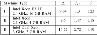
Our experiments measured the three attributes,∆,IR, andδ,
illustrating how accurately updates can be applied in software-based OpenFlow implementations. It should be noted that these three values depend on the processing power of the testbed machine; we measured the parameters for three types of DeterLab machines, Type I, II, and III, listed in Table II. Each attribute was measured 100 times on each machine type, and Fig. 8 illustrates our results. The figure graphically depicts the values∆,IR, andδof machine Type I as an example.
6An alternative representation of the accuracy, δ, assumes a symmetric
0 0.2 0.4 0.6 0.8 1 1.2 1.4
0.0085 0.0105 0.0125 0.0145 0.0165 0.0185
C
D
F
Time between two Controller Messages [seconds]
Type I Type II Type III ∆ [Type I]
(a) The empirical Cumulative Distribution Function (CDF) of the time elapsed between two consecutive controller messages.∆is the average value, which is shown in the figure for Type I.
0 0.2 0.4 0.6 0.8 1 1.2 1.4
0.006 0.008 0.01 0.012 0.014 0.016
C
D
F
Flow Installation Latency [seconds] Type I Type II Type III IR[Type I]
(b) The empirical CDF of the flow installation latency.IR is the difference between the max and min values, as shown in
the figure for Type I.
0 0.2 0.4 0.6 0.8 1 1.2 1.4
0 0.001 0.002 0.003 0.004 0.005
C
D
F
Scheduling Error [seconds]
Type I Type II Type III
δ [Type I]
(c) The empirical CDF of the scheduling error, i.e., the difference between the actual execution time and the scheduled execution time.δ is the maximal error value, as shown in the figure for Type I.
Fig. 8: Measurement of the three performance attributes: (a)∆, (b) IR, and (c)δ.
Machine Type ∆ IR δ
I Intel Xeon E3 LP 9.64 1.3 1.23 2.4 GHz, 16 GB RAM
II Intel Xeon 9.6 1.47 1.18 2.1 GHz, 4 GB RAM
II Intel Dual Xeon 14.27 2.72 1.19 3 GHz, 2 GB RAM
TABLE II: Measured attributes in milliseconds.
The measured scheduling error, δ, was slightly more than 1 millisecond in all the machines we tested. Our experiments showed that theclock accuracyusing REVERSEPTP over the DeterLab testbed is on the order of 100 microseconds. The measured value of δ in Table II shows the execution accu-racy, which is an order of magnitude higher. The installation latency range, IR, was slightly higher than δ, around 1 to 3
milliseconds. The measured value of∆was high, on the order of 10 milliseconds, as Dpctl is not optimized for performance. In software-based switches, the CPU handles both the data-plane traffic and the communication with the controller, and thusIRandδcan be affected by the rate of data-plane traffic
through the switch. Hence, in our experiments we fixed the rate of traffic through each switch to 10 Mbps, allowing an ‘apples-to-apples’ comparison between experiments.
C. Microbenchmark: Video Swapping
To demonstrate how TIME4 is used in a real-life scenario, we reconstructed the video swapping topology of [29], as illustrated in Fig. 9a. Two video cameras, A and B, transmit an uncompressed video stream to targets A and B, respectively. At a given point in time, the two video streams are swapped, so that the stream from source A is transmitted to target B, and the stream from B is sent to target A. As described in [29], the swap must be performed at a specific time instant, in which the video sources transmit data that is not visible to the viewer, making the swap unnoticeable.
The authors of [29] noted that the precisely-timed swap cannot be performed by an OpenFlow switch, as currently OpenFlow does not provide abstractions for performing ac-curately timed changes. Instead, it uses source timing, where
(a) Topology.
0 200 400 600 800 1000 1200 1400 1600 1800
-1.5 -0.5 0.5 1.5
Scheduling Error [milliseconds]
(b) Video swapping accuracy.
Fig. 9: Microbenchmark: video swapping.
sources A and B are time-synchronized, and determine the swap time by using a swap indication in the packet header. The OpenFlow switch acts upon the swap indication to determine the correct path for each stream. We note that the main drawback of this source-timed approach is that the SMPTE 2022-6 video streaming standard [56], which was used in [29], does not currently define an indication about where in the video stream a packet comes from, and specifically does not include an indication about the correct swapping time. Hence, off-the-shelf streaming equipment does not provide this indication. In [29], the authors used a dedicated Linux server to integrate the non-standard swap indication.
In this experiment we studied how TIME4 can tackle the video swapping scenario, avoiding the above drawback. Each node in the topology of Fig. 9a was emulated by a DeterLab machine. We used two 10 Mbps flows, generated by Iperf [57], to simulate the video streams. Each swap was initiated by the controller 100 milliseconds in advance (as in [29]): the controller sent a Scheduled Bundle, incorporating two updates, one for each of the flows. We repeated the experiment 100 times, and measured the scheduling error.
configuration, and every packet that was transmitted after
T was forwarded according to the new configuration. The scheduling error of each swap (measured in milliseconds) was computed as the number of misrouted packets, divided by the bandwidth of the traffic flow. The sign of the scheduling error indicates whether the swap was performed before the scheduled time (negative error) or after it (positive error).
Fig. 9b illustrates the empirical Probability Density Function (PDF) of the scheduling error of the swap, i.e., the difference between the actual swapping time and the scheduled swapping time. As shown in the figure, the swap is performed within ±0.6 milliseconds of the scheduled swap time. We note that this is the achievable accuracy in a software-based OpenFlow switch, and that a much higher degree of accuracy, on the order of microseconds, can be achieved if two conditions are met: (i) A hardware switch is used, supporting timed updates with a microsecond accuracy, as shown in [30], and (ii) The cameras are connected to the switch over a single hop, allowing low latency variation, on the order of microseconds.
D. Flow Swap Evaluation
1) Experiment Setting
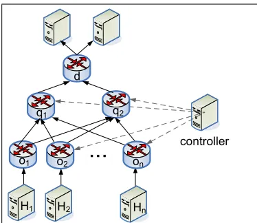
We evaluated our prototype on a 71-node testbed under. We used the testbed to emulate an OpenFlow network with 32 hosts and 32 leaf switches, as depicted in Fig. 11, with
n= 32.
controller
...
o1 o2 on
H1 H2 Hn
q1 q2
d
Fig. 11: Experimental evaluation: every host and switch was emulated by a Linux machine in the DeterLab testbed. All
links have a capacity of 10 Mbps. The controller is connected to the switches by an out-of-band network.
Metric.A flow swap that is not performed in a coordinated
way may bare a high cost: either packet loss, deep buffering, or a combination of the two. We use packet loss as a metric for the cost of flow swaps, assuming that deep buffering is not used.
We used Iperf to generate flows from the sources to the destination, and to measure the number of packets lost between the source and the destination.
The flow swap scenario.All experiments were flow swaps
with a swap impact of 0.5.7 We used two static flows,
7By Theorem 3, the source can force the controller to perform a flow swap
with an impact as high as roughly0.5.
which were not reconfigured in the experiment:H1 generates a5Mbps flow that is forwarded throughq1, andH2generates a5 Mbps flow that is generated through q2. We generated n additional flows (where n is the number of switches at the bottom layer of the graph): (i) A 5 Mbps flow from H1 to the destination. (ii)n−1 flows, each having a bandwidth of
5
n−1 Mbps. Every flow swap in our experiment required the flow of (i) to be swapped with the n−1 flows of (ii). Note that this swap has an impact of0.5.
2) Experimental Results
TIME4 vs. other update approaches. In this experiment
we compared the packet loss of TIME4 to other update approaches described in Sec. I-D. As discussed in Sec. I-D, applying theorderapproach or thetwo-phaseapproach to flow swaps produces similar results. This observation is illustrated in Fig. 10b. In the rest of this section we refer to these two approaches collectively as theuntimed approaches.
In our experiments we also implemented a SWAN-based [23] update, and a B4-SWAN-based [24] update. In SWAN, we used a 10% scratch on each of the links, and in B4 updates we temporarily reduced the bandwidth of each flow by 10% to avoid packet loss. As depicted in Fig. 10b, SWAN and B4 yield a slightly lower packet loss rate than TIME4; the average number of packets lost in each TIME4 flow swap is0.2, while with SWAN and B4 only0.1 packets are lost on average.
To study the effect of using time in SWAN and in B4, we also performed hybrid updates, illustrated in Fig. 10c and 10d, and in the two right-most bars of Fig. 10b. We combined SWAN and TIME4, by performing a timed update on a network with scratch capacity, and compared the packet loss to the conventional SWAN-based update. We repeated the experiment for various values of scratch capacity, from 0% to 10%. As illustrated in Fig. 10c, the TIME4+SWAN approach can achieve the same level of packet loss as SWAN with
less scratch capacity. We performed a similar experiment
with a timed B4 update, varying the bandwidth reduction rate between 0% and 10%, and observed similar results.
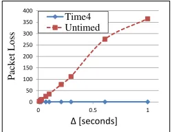
Number of switches. We evaluated the effect of n, the
number of switches involved in the flow swap, on the packet loss. We performed an n-swap with n = 2,4,8,16,32. As illustrated in Fig. 10a, the number of packets lost during an untimed update grows linearly with the number of switchesn, while the number of packets lost in a TIME4 update is less than one on average, and is not affected by the number of switches. As n increases, the update duration8 is longer, and
hence more packets are lost during the update procedure.
Controller performance. In this experiment we explored
how the controller’s performance, represented by ∆, affects the packet loss rate in an untimed update. As∆increases, the update procedure requires a longer period of time, and hence more packets are lost (Fig. 12) during the process. We note that although previous work has shown that∆can be on the order of microseconds in some cases [54], Dpctl is not optimized for performance, and hence∆ in our experiments was on the
8Theupdate durationis the time elapsed from the instant the first switch
0 5 10 15 20 25 30 35
0 10 20 30
P a c k e t L o s s
Number of switches
Time4 Untimed
(a) The no. of packets lost in a flow swap vs. no. of switches
involved in the update.
0.01 0.1 1 10 100
Order Two-phase Time4 B4 SWAN Time4B4 Time4SW
P a ck et L o ss ( lo g a ri th m ic ) B4 Time4SWTimed Untimed
(b) The number of packets lost in a flow swap in different update approaches
(withn= 32).
0 5 10 15 20 25 30 35 40
0 2 4 6 8 10
P a ck et L o ss
Scratch Capacity [%] Time4 + SWAN SWAN
(c) The number of packets lost in a flow swap using SWAN and TIME4+SWAN (withn= 32).
0 5 10 15 20 25 30 35 40
0 2 4 6 8 10
P a c k e t L o ss
Flow Bandwidth Reduction [%] Time4 + B4 B4
(d) The number of packets lost in a flow swap using B4 and TIME4+B4 (withn= 32).
Fig. 10: Flow swap performance: in large networks (a) TIME4 allows significantly less packet loss than untimed approaches. The packet loss of TIME4 is slightly higher than SWAN and B4 (b), while the latter two methods incur higher overhead. Combining TIME4 with SWAN or B4 provides the best of both worlds; low packet loss (b) and low overhead (c and d).
order of milliseconds. As shown in Fig. 12, we synthetically increased ∆, and observed its effect on the packet loss during flow swaps. 0 50 100 150 200 250 300 350 400
0 0.5 1
P a c k e t L o s s Δ [seconds] Time4 Untimed
Fig. 12: The number of packets lost in a flow swap vs.∆. The packet loss in TIME4 is not affected by the controller’s
performance (∆).
Installation latency variation. Our next experiment
(Fig. 13a) examined how the installation latency variation, denoted by IR, affects the packet loss during an untimed
update. We analyzed different values ofIR: in each update we
synthetically determined a uniformly distributed installation latency, I ∼ U[0, IR]. As shown in Fig. 13a, the switch’s
installation latency range, IR, dramatically affects the packet
loss rate during an untimed update. Notably, whenIRis on the
order of 1 second, as in the extreme scenarios of [28], [55], TIME4 has a significant advantage over the untimed approach.
Scheduling error. Figure 13b depicts the packet loss as a
function of the scheduling error of TIME4. By Fig. 10a, 13a and 13b, we observe that if δ is sufficiently low compared to IR and (n−1)∆, then TIME4 outperforms the untimed
approaches. Note that even if switches are not implemented with extremely low scheduling error δ, we expect TIME4 to outperform the untimed approach, as typically δ < IR, as
further discussed in Section V.
Summary. The experiments presented in this section
demonstrate that TIME4 performs significantly better than untimed approaches, especially when the update involves mul-tiple switches, or when there is a non-deterministic installation latency. Interestingly, TIME4 can be used in conjunction with existing approaches, such as SWAN and B4, allowing the same level of packet loss with less overhead than the untimed
0 20 40 60 80 100 120 140 160
0 0.5 1
P a c k e t L o ss
IR[seconds] Untimed
(a) The number of packets lost in a flow swap vs. the installation latency range,IR.
0 20 40 60 80 100 120 140 160
0 0.5 1
P a c k e t L o ss
δ [seconds] Time4
(b) The number of packets lost in a flow swap vs. the
scheduling error,δ.
Fig. 13: Performance as a function of IR and δ. Untimed
updates are affected by the installation latency variation (IR),
whereas TIME4 is affected by the scheduling error (δ). TIME4 is advantageous since typicallyδ < IR.
variants.
V. DISCUSSION
1) Scheduling accuracy
The advantage of timed updates greatly depends on the
scheduling accuracy, i.e., on the switches’ ability to
accu-rately perform an update at its scheduled time. Clocks can typ-ically be synchronized on the order of1microsecond (e.g., [6]) using PTP [5]. However, a switch’s ability to accurately perform a scheduled action depends on its implementation.
• Software switches: Our experimental evaluation showed that the scheduling error in the software switches we tested was on the order of 1 millisecond.
• Hardware-based scheduling:The work of [30] has shown a method that allows the scheduling error of timed events in hardware switches to be as low as 1 microsecond. • Software-based scheduling in hardware switches: A
scheduling mechanism that relies on the switch’s software may be affected by the switch’s operating system and by other running tasks. Measures can be taken to implement an accurate software-based scheduling in TIME4: when a switch is aware of an update that is scheduled to take place at time Ts, it can avoid performing heavy
rearrangement. Update messages received slightly before timeTscan be queued and processed after the scheduled
update is executed. Moreover, if a switch receives a timed command that is scheduled to take place at the same time as a previously received command, it can send an error message to the controller, indicating that the last received command cannot be executed.
It is an important observation that in a typical system we expect the scheduling error to be lower than the installation latency variation, i.e., δ < IR. Untimed updates have a
non-deterministic installation latency. On the other hand, timed updates are predictable, and can be scheduled in a way that avoids conflicts between multiple updates, allowing δ to be typically lower than IR.
2) Model assumptions
Our model assumes a lossless network with unsplittable,
fixed-bandwidthflows. A notable example of a setting in which these assumptions are often valid is a WAN or a carrier network. In carrier networks the maximal bandwidth of a service is defined by its bandwidth profile [27]. Thus, the controller cannot dynamically change the bandwidth of the flows, as they are determined by the SLA. The Frame Loss Ratio (FLR) is one of the key performance attributes [27] that a service provider must comply to, and cannot be compromised.
Splitting a flow between two or more paths may result in
packets being received out-of-order. Packet reordering is a key performance parameter in carrier-grade performance and availability measurement, as it affects various applications such as real-time media streaming [58]. Thus, all packets of a flow are forwarded through the same path.
3) Short term vs. long term scheduling
The OpenFlow time extension we presented in Section III is intended for short term scheduling; a controller should schedule an action to a near-future time, on the order of seconds in the future. The challenge in long term scheduling is that during the long period between the time at which the Scheduled Bundle was sent and the time at which it is meant to be executed various external events may occur: the controller may fail or reboot, or a second controller9may try to perform
a conflicting update. Near future scheduling guarantees that external events that may affect the scheduled operation such as a switch reboot have a low probability of occurring. Since near-future scheduling is on the order of seconds, this short potentially hazardous period is no worse than in conventional updates, where an OpenFlow command may be executed a few seconds after it was sent by the controller.
4) Network latency
In Fig. 1, the switches S1 andS3 are updated at the same time, as it is implicitly assumed that all the links have the same latency. In the general case each link has a different latency, and thus S1 andS3 should not be updated at the same time, but at two different times, T1 and T3, that account for the different latencies.
9In an SDN with a distributed control plane, where more than one controller
is used.
5) Failures
A timed update may fail to be performed in a coordinated way at multiple switches if some of the switches have failed, or if some of the controller commands have failed to reach some of the switches. Therefore, the controller uses a reliable transport protocol (TCP), in which dropped packets are re-transmitted. If the controller detects that a switch has failed, or failed to receive some of the Bundle messages, the controller can use theBundle Discardto cancel the coordinated update. Note that the controller should send timed update messages sufficiently ahead of the scheduled time of execution, allowing enough time for possible retransmission and Discard message transmission.
6) Controller performance overhead
The prototype design we presented (Fig. 7) uses RE-VERSEPTP [46] to synchronize the switch and the controllers. A synchronization protocol may yield some performance over-head on the controller and switches, and some overover-head on the network bandwidth. In our experiments we observed that the CPU utilization of the PTP processes in the controller in an experiment with 32 switches was5%on the weakest machine we tested, and significantly less than 1% on the stronger machines. As for the network bandwidth overhead, accurate synchronization using PTP typically requires the controller to exchange∼5packets per second per switch [59], a negligible overhead in high-speed networks.
VI. CONCLUSION
Time and clocks are valuable tools for coordinating up-dates in a network. We have shown that dynamic traffic steering by SDN controllers requires flow swaps, which are best performed as close to instantaneously as possible. Time-based operation can help to achieve carrier-grade packet loss rate in environments that require rapid path reconfiguration. Our OpenFlow time extension can be used for implementing flow swaps and TIME4. It can also be used for a variety of additional timed update scenarios that can help improve network performance during path and policy updates.
VII. ACKNOWLEDGMENTS