Vol. 2, No. 2, Fall 2013, 47-69
Total Factor Productivity Growth, Technical Change and Technical Efficiency Change in Asian Economies:
Decomposition Analysis
Vahid Shahabinejad∗♣ Baft Higher Education Center, Shahid
Bahonar University of Kerman,Iran [email protected]
Mohammad Reza Zare Mehrjerdi Department of Agricultural Economics Shahid Bahonar University of Kerman,Iran
[email protected] Morteza Yaghoubi
Department of Agricultural Economics University of Sistan and Baluchistan (USB)
Abstract
The aim of this paper is to analyze total factor productivity (TFP) growth and its components in Asian countries applying Stochastic Frontier Analysis (SFA) to the time series data of 44 Asian countries from 2000 to 2010. Using Battese and Coelli approach, TFP is divided into technical efficiency change and technical change. TFP decomposition using SFA method for the years 1998 to 2007 indicates that in 75 % of these economies, the role of technical change in productivity growth is negative. Only in 11 countries technical change had a positive role in productivity growth. The growth of TFP shows that Japan has the highest productivity growth (2.55 %) and Saudi Arabia, Korea and Hong Kong are located in subsequent positions. Furthermore, due to the lowest technical progress, newly independent countries, such as Armenia, Azerbaijan, Kazakhstan, Kyrgyzstan, Tajikistan, Turkmenistan and Uzbekistan have the slowest TFP growth.
Keywords: Efficiency, Productivity, Technical progress, Stochastic Frontier Analysis (SFA), Asian Economies.
JEL Classification: C23, D24, O47, Q32, R11, O39.
Received: 20/4/2013 Accepted: 13/7/2014 ∗ The Corresponding author
♣ Acknowledgement
1.Introduction
Accumulation of production factors and productivity growth are among the major determinants of economic growth. Due to the scarceness of available resources, it is essential to consider other approaches toward development, especially efficiency and TFP. Productivity is a comprehensive concept and refers to the effective and efficient use of resources to obtain the highest and best output (Hejazi et al, 2008). Efficiency is an economic concept which shows the performance of a wide range of economic activities within a firm or a sector of the economy (Hakimi & Hozhbrkiani, 2008). It is reported that most of the developed countries gain a high percentage of their economic growth by increasing TFP. To make it clear we can mention USA which had 48%TFP growth during 1953 to 1969. However, the share of the capital stock and labor force growth was respectively 22% and 33%, (Shah Abadi, 2010). From 1994 to 1960, average annual growth of TFP has been 2.81% in Japan which composed of 53% of economic growth in this country (Hunma, 2001). During the same period, the average of South Korea's annual GDP growth has been 7.3 % out of which 44.53 percent was due to growth TFP (Lee, 2001). In Indonesia, the rate of productivity growth in its economic growth was -4% from 1970 to 2007 that demonstrates the negative impact of productivity growth in economic growth of this country (Van der Eng, 2009). Also in Philippines the share of productivity growth from economic growth is obtained -6.8 percent (Silva, 2001). According to a research conducted by Alimoradi et al, 2003, the average annual growth of TFP in Iran was approximately -8.12% from1966to 2000.They reported 10.8% of annual growth in labor force input and 1.83% of annual growth in capital input.
because of not having access to the data to determine the share and the price of labor force and capital in GNP. In this study, we aim to determine the productivity growth of Asian countries. Therefore we could compare these countries based on their productivity growth as well, as we specify the countries that obtained a portion of their economic growth by their TFP. Moreover, we tried to analyze productivity into two components: analysis of technical progress and changes in technical efficiency to determine the main factor of productivity growth in each country.
2. Literature Review
This paper uses an alternative way of measuring total factor productivity based on the analysis of stochastic frontiers. The great advantage of this approach is the possibility that it offers for decomposing productivity change into parts that can have a straightforward and simple economic interpretation. The stochastic frontier model used assumes the existence of technical inefficiency which evolves following a particular behavior. These assumptions allow one to split productivity changes into two parts. The first is the change in technical efficiency, which measures the movement of an economy towards the production frontier; the second is technical progress, which measures shifts of the frontier over time. The SFA has been used in many articles; some of which are mentioned here:
growth. Their results also indicate both economic freedom and ethnic homogeneity help growth. More, Azomahou et al (2013) studied the productivity growth of both developed and developing countries by applying a semi-parametric generalized additive model over the period of 1998–2008 and determined the relation among the productivity growth and the world productivity growth, human capital, total staff in R&D, the share of R&D expenditure, the increase in government spending on R&D and international trade. In addition, Ilmakunnas and Miyakoshi (2013) explored the TFP based on the quality of the labor and capital inputs in the manufacturing industries of some OECD countries and suggested two labor and ICT indexes to find some specific impacts on productivity.
Afonso and Aubyn (2010) estimated total factor productivity of OECD countries by using stochastic frontier and data envelopment analysis. The results indicated Belgium, Canada, Spain, Italy, Japan and Portugal have been more efficient. The results obtained from using TFP, technical efficiency and technical changes show that on average, there is a positive growth in TFP growth; however the contribution of technical efficiency is more than technical progress. The results of DEA method confirm the results of SFA for a large number of countries, as well.
country as the non-member countries had a positive technical progress. Deliktas (2008) compared technical efficiency and productivity growth of the Countries of the former Soviet Union before and after the collapse. Using DEA, total productivity changes and its components were estimated. The results of this study show that after the collapse, these countries averagely have had the technical efficiency growth of positive, but the technological and total productivity of negative. These results for pre-collapse are almost the reverse so that the average technical efficiency growth in these countries is negative, while the growth rate of technical progress in these countries averagely is positive.
Han et al. (2002) using the stochastic frontier approach estimated 20 production function industry in Hong Kong, Japan, Singapore and South Korea in 1987-1993.
Overall, these results indicate the importance of growth factors in the economy of these countries. Changes in technology have had a greater share of the economic growth compared to the technical efficiency. In Hong Kong, however technological changes for most counties have been positive but because of inefficiency effects, total productivity growth has been negative. In Japan, technical efficiency changes have been positive for all 20 industries while, technical progress has been negative. But since technical efficiency changes compared to technical progress have been negligible, TFP growth of Japan has been negative and the main factor of economic growth has been input growth as well. Singapore has been better placed than Japan in terms of the economic growth and development but has a similar rate in terms of factors growth. In South Korea averagely half of these industries have experienced positive changes in technical efficiency, while technological advances have occurred in most industrial countries. Thus, in this country TFP growth has been positive. Thus like the three above, the main factor of economic growth in the period under review has been the accumulation of factors of production.
3.Methodology 3.1 Accounting for inefficiency
using a stochastic frontier model. Supposing that a country has a production function , , in a word without error or inefficiency, in time t, the ith country would produce
, (1)
A fundamental element of stochastic frontier analysis is that each country potentially produces less than it might because of a degree of inefficiency. Specifically,
, ζ (2)
Whereζ is the level of efficiency for country i at time t; ζ must be in the interval 0,1 . ζ 1means the country is achieving the optimal output with the technology embodied in the production function f Z , β
andζ 1 indicates , the country is not able to maximize the using of inputs Z given the technology embodied in the production function
f Z , β because the output is assumed to be strictly positive (i.e.,q 0, the degree of technical efficiency is assumed to be strictly positive (i.e.,ζ 0).
Output is assumed to be subject to random shocks, implying that
, ζ (3)
Taking the natural log of both sides yields
, ζ (4)
Assuming that there are k inputs and that the production functions is linear in logs, defining
ζ Yields ∑ (5)
Because u is subtracted from ln q , restricting u 0 implies that0 ζ 1, as specified above.
In the time invariant model, , u ~N µ, σ ,v ~N 0, σ , and u
In the time-varying decay specification, according to parameterization formulated by Battese & Coelli (1992):
η η , (6)
Where T is the last period in the th panel,η is the decay parameter and represents the rate of change in technical inefficiency and the non-negative random variable u is the technical inefficiency effects for the i-th country in i-the last year for i-the dataset. That is, i-the technical inefficiency effects in earlier periods are a deterministic exponential function of the inefficiency effects for the corresponding forms in the final period (i.e. u u given that data for the i'th country available in period T). τ i is the set of T periods and may contain all periods in the panel or only a subset of periods [Pires & Garcia, 2004].
The sign of µ indicates the trend of technical inefficiency that does not vary in time. When µ is not significantly different from zero, we have technical inefficiency that does not vary in time also called persistent inefficiency. If µ is positive, then η η is positive for and so η 1, which implies that the technical inefficiencies of countries decline over time. If µ is negative, thenη 0 and thus the technical inefficiencies of countries increase over time.
3.2 Decomposition of TFP
change and technological change as component of productivity change, which introduces an additional dimension to the analysis from the policy perspective (Nishimizu & page, 1982; Bayarsaihan, Battese & Coelli, 1998).
We define this so called best practice function f (0) as,
y , (7)
Where y is the potential output level on the frontier at time t for production unit i, given technology f(.), and x is a vector of inputs. Take log and totally differentiate (1) with respect to time to get
, ,
∑ , . ∑ (8)
Where the first term on the right-hand side is the output elasticity of frontier output with respect to time, defined as TP, the second term measures the input growth weighted by output elasticity’s with respect to input j, , . Note that the conventional conceptualization of TFP growth can be defined as output growth unexplained by input growth, i.e.
∑ (9)
Combining equation (7) and (8), one can get
∑ , (10)
That is TP is the only source of TFP growth.
In the spirit of Nishimizu & Page (1982) and further frontier analysis, any observed output using for input can be expressed as, [Liao et al. 2006]
, (11)
random variation across production unit and random shocks that are external to its control. Regarding (10),
Growth rate of is calculated as below (Liao et al, 2006):
, ∑
(12)
From equation (11), TFP growth consists of two components: technical change (innovation and shifts in the frontier technology) and technical efficiency change (catching-up), that is,
(13)
0 Represents an upward shift of the production frontier. If the technology is immutable, it does not contribute in any way to productivity gains. The same happens with technical inefficiency. If it does not vary overtime, it also does not have any impact on the rate of variation of productivity [Pires & Garcia, 2004].This decomposition of TFP growth is useful in distinguishing innovation or adoption of new technology by ‘best practice’ production units from the diffusion of technology. Coexistence of a high rate of TP and a low rate of change in technical efficiency may reflect the failures in achieving technological mastery or diffusion (Kalirajan, Obwona & Zhao, 1996).
3.3 Model specification
To operationalize the model in equations (5) in our empirical analysis we need to specify a functional form. Following Kumbhakar and Wang (2005), we prefer a translog specification over a Cobb-Douglas specification due to the latter’s superior flexibility [Duffy and Papageorgiou, 2000]. Unlike Koop et al. (1999, 2000), we explicitly account for technology shifts in the frontier. That is, we include a trend variable t with interaction terms that allows us to identify the contribution of technological change to TFP growth. The reduced form of equation is then:
(14)
Rather than pursuing a mathematical programming approach, such as DEA Malmquist Index which is deterministic in nature (as do Fare et al. 1985; Fare et al 1994; etc). It is easy to debate the relative merits of this way, including its grounding in economic theory, the flexibility of translog from less sensitive to extreme observations and measurement error or rather statistical noise in the data due to modeled distributions of errors and efficiency, and so on (Sharma, Leung & Zaleski, 1997). For the case of agricultural and manufacturing application in developing countries, stochastic frontier analysis are likely to be more appropriate than DEA where the data are heavily influenced by measurement error.
The above specification allows the estimation of the both TP in the stochastic frontier and time-varying technical efficiency. Note that the translog parameterization of this stochastic frontier model allows for non-neutral TP. TP is non-neutral if all s are equal to zero. The production function reduces to the Cobb-Douglas function with neutral TP if all the s is equal to zero.
The distribution and parameterization of technical efficiency effects
u were discussed above.
Since the estimation of technical efficiency are sensitive to the choice of distribution assumption, we consider truncated normal distribution for general specifications for one-sided error u , and half- normal distribution can be tested by LR test. The technical efficiency level of unit i at time t is then defined as the ratio of the actual output to the potential output,
(15)
And TEC is the change in TE, and the rate of technical progress is defined by,
,
(16)
production function with respect to time.
3.4 Data specification
We construct a non-balanced panel data set consisting of 44 Asian countries over the period 1972-2010. The output variable is GDP measured at constant prices (2005 US$). It is obtained by taking the real GDP per capita chain series (rgdpch) from PWT6.3 and multiplying it by total population for each country.
With respect to labor we use a proxy, the population of equivalent adults (peqa), obtained from PWT (Penn world Table). These data are obtained indirectly from the PWT6.3, by performing calculation using three variables:
. . . (17)
Where rgdpch is the real GDP per capita chain series (rgdpch), rgdpeqa is real GDP per equivalent adult and pop is population.
The standard perpetual inventory method (PIM) is used here to construct the capital stock under a uniform 6% depreciation rate with 1970 as the reference year
K, K, I, δ , (18)
Where K, is capital stock of country i at period t, I, is capital formation
and δ is depreciation rate. Following Hall & John (1996), the initial capital stock series is initialized by assuming that the growth rate of investment series is representative of the growth of investment prior to the beginning of the series. That is,
∑
∑
∞ = − − ∞ = −− − = + − = += 0 1 ,0
0 , 0 , 1
i,0 (1 ) (1 ) (1 ) ( )
K t i i t t i j t t t j g I g I
I δ δ δ (19)
4. Empirical Results
In this section we report specification tests, discuss efficiency, technical progress and TFP growth levels, also provide TFP decomposition.
4.1 Estimation of the Asian stochastic frontier (1972-2010)
The STATA11 software which includes among its preprogrammed models of Battese and Coelli (1992) was used to estimate the model and TFP decomposition.
Parameters presented in Table 1 are all significant at 1%. The mean inefficiencyµ is significantly different from zero at 1%, showing that normal truncated distribution is an appropriate assumption (if it were not significant other case of distribution must be tested). The estimated value of ηis positive, which means technical efficiency growth at decreasing rates (catch up).
Table1: Time variant inefficiency model
Time-varying decay inefficiency model Number of obs =1474 Group variable: id Number of groups = 44 Time variable: t Obs per group: min = 15
Avg =33.5 Max = 38 Wald chi2 (9) = 8854.64 Log likelihood = 199.31833 Prob > chi2 = 0.0000
LnY Coef Std. Err. Z p>⏐z⏐ [95% Conf. Interval]
T -.104766 .0150332 -6.97 0.000 -.134231 -.075302 Lnk -.807525 .1824968 -4.42 0.000 -1.16521 -.449838 Lnl .5556781 .1614806 3.44 0.001 .239182 .8721741 t2 .0012097 .0001296 9.34 0.000 .0009557 .0014636 lnk2 .0852134 .010201 8.35 0.000 .0652199 .1052069 lnl2 .1762944 .0165895 10.63 0.000 .1437796 .2088091 Lnklnl -.156111 .0208135 -7.50 0.000 -.196905 -.115318
Tlnk .0035676 .0006806 5.24 0.000 .0022337 .0049016 Tlnl -.002972 .0008431 -3.53 0.000 -.004624 -.001319 Cons 24.28848 1.863513 13.03 0.000 20.63606 27.9409
Mu .686165 .1414601 4.85 0.000 .4089083 .9634218 Eta .0228559 .0011867 19.26 0.000 .0205299 .0251818 lnsigma2 -1.06112 .3112756 -3.41 0.001 -1.67121 -.451036 Ilgtgamma 2.110568 .3512403 6.01 0.000 1.42215 2.798987
4.2 The results of the hypothesis tests
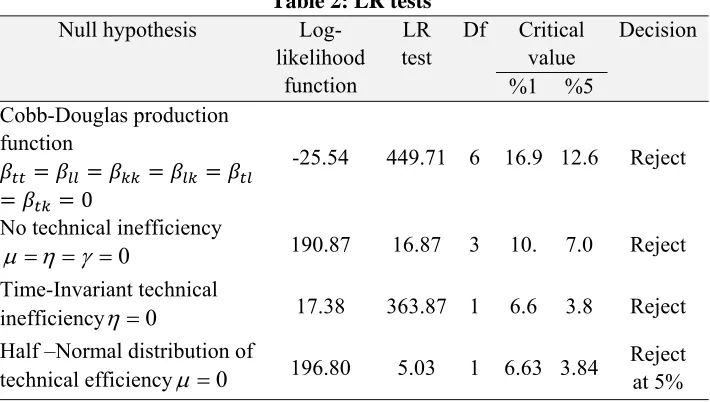
Since this study is going to compare the productivity and efficiency by using frontiers and production functions approaches, it is necessary to consider some related hypothesis. All hypotheses are tested on two significant levels of 1% and 5% by applying generalized maximum likelihood method (relation 8). The results are shown in Table 2.
Table 2: LR tests
Decision Critical value Df LR test Log-likelihood function Null hypothesis %5 %1 Reject 12.6 16.9 6 449.71 -25.54 Cobb-Douglas production function 0 Reject 7.0 10. 3 16.87 190.87
No technical inefficiency 0
µ η γ= = =
Reject 3.8 6.6 1 363.87 17.38 Time-Invariant technical inefficiencyη=0
Reject at 5% 3.84 6.63 1 5.03 196.80
Half –Normal distribution of technical efficiencyµ =0
First we test whether Cobb-Douglas production function are adequate to describe underlying technology. The hypothesis is rejected; therefore Translog function form is preferred to a Cobb-Douglas specification.
The second assumption considers the effect of technological changes. In other words, the neutrality of technological changes which names Hicks neutral technological change, as well, is examined.
The third and most important assumption is related to the absence of technical inefficiency in the model. In this assumption signifying the parameters η ،µandγ , µ η γ= = =0is simultaneously tested (Liao et al, 2006). The rejection of this assumption means inefficiency.
will change overtime.
Fifth assumption is related to the type of distribution of technical inefficiency and the rejection of H0 = =
µ
0means that the type of distribution is appropriate. However, the last two assumptions of the results of the model can decide the acceptance or rejection of them so that according to the coefficients, these assumptions are not accepted.4.3 The results of productivity analysis using stochastic method
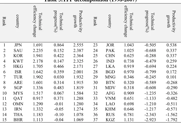
The results of calculation in Table 3 show that Japan, Saudi Arabia, South Korea, Kuwait and Hong Kong are on the top and newly independent countries are at the bottom of the Table. Ranking of countries in the Table is based on productivity growth. The results show that in a decade, 2000- 2010, countries in terms of productivity growth are generally divided into two groups: Countries with positive productivity growth and countries with negative productivity growth.
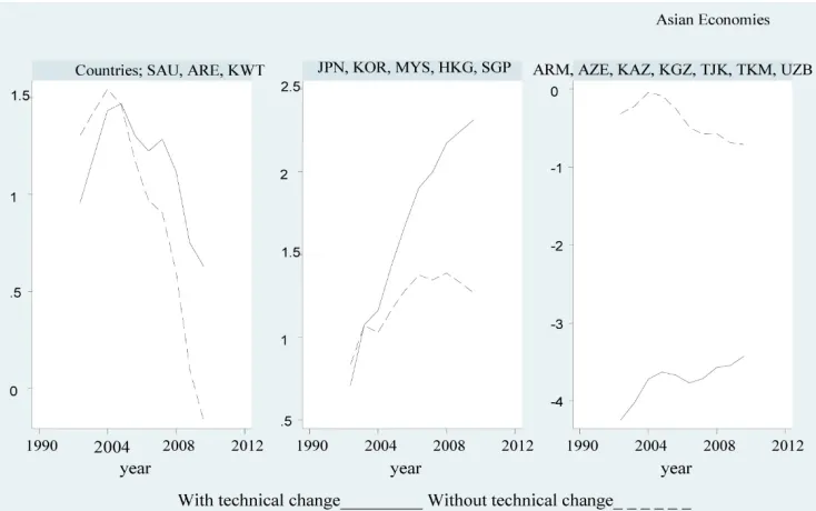
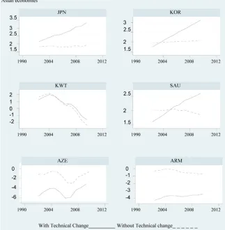
In some countries there are positive productivity growth, both the efficiency change and technical progress lead to improve productivity. These include: Among the countries where productivity growth is positive both Saudi Arabia and Kuwait have achieved greater share of productivity growth through changes in technical efficiency, while technical progress in these countries compared to East Asian countries Japan, Singapore, South Korea and Hong Kong was lower. As shown in Graph 1 and Graph 2, in East Asian countries such as Japan, Korea, Malaysia, Hong Kong and Singapore technology changes have had a great effect on the productivity growth. In Saudi Arabia, Kuwait and the UAE, changes in technology have had a positive impact on the productivity growth but are lower than Asian countries.
Figure 1. TFP growth in selected countries, with and without technical change (2000-2010)
factor of TFP growth are Oman, Thailand, Bahrain, Syria, Indonesia, Lebanon, the Philippines, Iraq, Jordan, Pakistan, China, India, Sri Lanka, Bangladesh and Mongolia.
In countries where average productivity growth was negative, the main factor of negative growth in productivity has been negative changes
in technology. However, this point should not be forgotten that technical efficiency of all these countries has been on average less than one but technology changes are negative in most of these countries so that even
the best countries in terms of performance, cannot compensate for it.
Figure 2. TFP Growth, with and without technical change (2000-2010)
Uzbekistan, Azerbaijan, Turkmenistan, Armenia and Tajikistan in this group, as shown in Graph 1 and 2 are interesting due to negative changes in technology. However, due to significant capital losses in these countries, in the first half of 1990, the result is not unexpected. Taskin and Zaim (1997) Deliktas and Balcilar (2005) and Angeriz et al. (2006) have noted this point.
Furthermore, technological progress and changes in technical efficiency and productivity analysis indicated that 70% of these countries have been faced with negative technical progress. In other words, technical progress has a negative role in productivity growth in many countries, while the performance of all countries has a positive role in productivity growth. Japan, Singapore, Hong Kong and South Korea have the highest technical progress and the newly independent countries of Kazakhstan, Turkmenistan, Azerbaijan, Armenia and Tajikistan have the lowest rank.
4.4 Decomposition results
Table 3.TFP decomposition (1998-2007)
Rank country Techn
ica l effic iency ch ang e Techn ica l
progress(%) Productivity
growth Rank country Techn
ica l effic iency ch ang e Techn ica l
progress(%) Productivity
growth
Rank country Techn ica l effic iency ch ang e Techn ica l
progress(%) Productivity
growth Rank country Techn
ica l effic iency ch ang e Techn ica l
progress(%) Productivity
growth
16 CYP 0.963 0.091 1.054 38 KAZ 0.919 -3.266 -2.347 17 MAC 0.836 0.098 0.934 39 UZB 0.551 -2.989 -2.438 18 SYR 1.308 -0.54 0.765 40 YEM 0.665 -3.255 -2.589 19 IDN 1.156 -0.40 0.747 41 AZE 0.555 -3.600 -3.045 20 LBN 1.138 -0.46 0.670 42 TKM 0.389 -3.512 -3.123 21 PHL 1.209 -0.54 0.662 43 ARM 0.505 -3.843 -3.339 22 IRQ 1.400 -0.79 0.607 44 TJK 0.373 -4.215 -3.842
The significant point of calculating the technical change efficiency is that Saudi Arabia and Kuwait have the highest rank with an average equal 2.23 and 2.17 respectively and the newly independent countries of Azerbaijan, Uzbekistan, Armenia, Turkmenistan, Tajikistan and Mongolia follow consecutive that probably is due to similar economic structures after the formation of the Union commonwealth countries.
Figure 3. Technical efficiency change and technical progress (%) of economics of Asian countries for 10-year periods from 1998 to 2007. -۵ -۴ -٣ -٢ -١ ٠ ١ ٢
٣ JPN SAU KOR KWT HKG ISR TUR ARE SGP MYS QAT OMN IRN THA BH
R
Figure 4. TFP change of Asian countries economics for 10-year periods from 1998 to 2007
Access to the high growth rate of productivity is not easy and needs taking optimal use of all facilities and resources.
5. Conclusion
The results of this study demonstrated that there are two groups of countries in terms of productivity growth: Countries with positive productivity growth and countries with negative productivity growth. Japan with an average growth of 2.55% ranked first among other countries which was a result of its considerable technical progress. Saudi Arabia, South Korea, Kuwait and Hong Kong were in the latter ranks. However, Saudi Arabia and Kuwait had most of their productivity growth for the sake of changes in technical efficiency; while the technical progress of these two countries was lower than the East Asian countries such as Japan, Singapore, South Korea and Hong Kong.
In some countries despite the fact that the average of technical change was negative, yet due to the relatively high efficiency changes, productivity growth has been positive. In other words, efficiency changes have been the main factor of productivity growth in these countries. Iran is in this group as well. These countries were Oman, Iran, Thailand, Bahrain, Syria, Indonesia, Lebanon, the Philippines, Iraq, Jordan,
-۵
-۴
-٣
-٢
-١
٠ ١ ٢
٣ JPN SAU KOR KWT HKG ISR TUR ARE SGP MYS QAT OMN IRN THA BH
R
Pakistan, China, India, Sri Lanka, Bangladesh and Mongolia
In some countries, the main reason for negative productivity growth has been the result of negative changes of technology. These changes were negative in Russia, Kazakhstan, Turkmenistan, Azerbaijan, Armenia, Uzbekistan and Tajikistan and were relatively high. However, it should be considered that the average of technical efficiency has been lower than one in all of these countries. But in many countries, negative technical changes were in such a way that cause a negative growth of total productivity. Furthermore, division of productivity into technical efficiency and technological change showed that changes of efficiency in all countries had a positive impact on productivity growth whereas the role of technical progress has been negative.
References
Afonso, A., & St. Aubyn, M. (2010). Public and Private Inputs in Aggregate Production and Growth: A cross-country efficiency Approach; Working Paper Series, No. 1154.
Aigner Dennis J., Knox Lovell, C. A. & Schmidt, P. (1977). Formulation and Estimation of Stochastic Frontier Production Function Models. Journal of Econometrics, 6 (1), p21-37.
Aisen, A., & Veiga, F. J. (2013). How does political instability affect economic growth? European Journal of Political Economy, 29, 151-167.
Alimoradi, L., Shirin Bakhsh, S., & Totonchian, I. (2003). Measuring total factor productivity growth in the economy and determine its contribution to GDP growth, M.A. Dissertation, ALzahra university. Angeriz A., Mc Combie J., & Roberts, M. (2006). Productivity,
Efficiency and Technological Change in European Union Regional Manufacturing, A Data Envelopment Analysis Approach, the Manchester School 74(4), 500-525.
Arazmuradov, A., Martini, G., & Scotti, D. (2013). Determinants of total factor productivity in former Soviet Union economies: A stochastic frontier approach. Economic Systems.
Change and Economic Dynamics, 24, 45-75.
Baten, M. A., Kamil, A. A., & Kanis, F. (2009). Technical efficiency in Stochastic Frontier Production Model: An application to the
Manufacturing industry in Bangladesh. Australian Journal of Basic and Applied Sciences, 3(2): 1160-1169.
Battese, G., & Coelli, T. (1992). Frontier production functions, technical efficiency and panel data: With application to paddy farmers in India; Journal of Productivity Analysis, 3, 153-169.
Battese, G., & Coelli, T. (1995). A model for technical inefficiency effects in a Stochastic Frontier Production Function for Panel Data. Empirical Economics, 20, 325-332.
Bauer, P. W. (1990). Decomposing TFP in the presence of cost inefficiency, no constant returns to scale, and technological progress. Journal of Productivity Analysis, 1, 287-299.
Bayarsaihan, T., Battese, G. E., & Coelli, T. J. (1998). Productivity of Mongolian Grain Farming, CEPA Working Papers, No. 2/98, 1976-89.
Deliktas, E., & Balcilar, M. (2005). A Comparative analysis of productivity growth, catch-up and convergence in transition economies. Emerging Markets Finance and Trade, 41(1), 6-28. Deliktaş, E. (2008). The comparison of technical efficiency and
productivity growth in the former Soviet Countries for two periods, 3rd IEU-SUNY, Cortland Intern. Conf. in Economics, Economic Issues in Globalizing World, May 1-2, İzmir - Turkey.
Duffy, J., & Papageorgiou, C. ( 2000). A Crosscountry Empirical Investigation of the Aggregate Production Function Specification, Journal of Economic Growth , pp. 87-120.
Färe, R., Grosskopf, S., & Lovell, C. A. K. (1994). Production Frontiers. Cambridge, UK, Cambridge University Press.
Färe, R., Grosskopf, S. & Lovell, C. A. K. (1985). The Measurement of Efficiency of Production, Boston: Kluwer-Nijh off Publishing. Hall, R., & Jones, C. (1996). The productivity of nations. NBER Working
Paper no. 5812.
Knowledge and Development, 15(24), 133-161.
Han, G., Kalirajan. K. P., & Singh, N. (2001). Productivity and Economic Growth in East Asia: Innovation, Efficiency and Accumulation; Santa Cruz Center for International Economics Working Paper ,01-2.
Hejazi, R., Anvari Rostami, A., & Moghadasi, M. (2008). Total productivity analysis of export development bank of Iran and productivity growth in branches. Journal of Industrial Management, 1(1), 39-50.
Honma, M. (2001). Measuring Total Factor Productivity in Japan. Measuring Total Factor Productivity. Tokyo: Asian Productivity Organization. 81.
Ilmakunnas, P., & Miyakoshi, T. (2013). What are the drivers of TFP in the Aging Economy? Aging labor and ICT capital. Journal of Comparative Economics, 41(1), 201-211.
Kalirajan, K. P., Obwona, M. B., & Zha S. ( 1996). A decomposition of total factor productivity growth: the case of Chinese agricultural growth before and after reforms. American Journal of Agricultural Economics, 78, pp 331-338.
Koop, G., Osiewalski, J., & Steel, M. F. J. (1999). The components of output growth: a stochastic frontier analysis. Oxford Bulletin of Economics and Statistics, 61,pp 455-487.
Kumbhakar, S. C., & Lovell, C. A. K. (2000). Stochastic Frontier Analysis, Cambridge University Press, Cambridge, UK.
Kumbhakar, S. C., & Wang, Hung-Jen (2005). Estimation of growth convergence using a stochastic production frontier approach, Economics Letters, Elsevier, 88(3), pages 300-305.
Lee, B. (2001). Measuring Total Factor Productivity in Republic of Korea. Measuring Total Factor Productivity; Tokyo: Asian Productivity Organization, p: 100.
Liao, H., Holmes, M., Weyman-Jones, T., & Llewellyn, D. (2006). Productivity growth of East Asia economies’ manufacturing: a decomposition analysis. Journal of Development Studies, 43(4), pp 649-674.
Cobb–Douglas production functions with composed error; International Economic Review, 18: 435–444.
Nishimizu, M., & Page J. M. (1982). Total factor productivity growth, technological progress and technical efficiency change: dimensions of productivity change in Yugoslavia, 1965-78. Economic Journal, 92, pp 920-936.
Pires, J. O., & Garcia, F. (2004). Productivity of Nation: A Stochastic Frontier Approach to TFP Decomposition. Economia Rev, 143. Rath, BN & Madheswaran, S. (2004). Productivity growth of Indian
manufacturing sector: Panel estimation of stochastic production frontier and technical inefficiency. In Econometric Society 2004 Far Eastern Meetings (No. 527). Econometric Society.
Salinas Jimenez, J., & Salinas Jimenez, M. (2007). Corruption, Efficiency and Productivity in OECD Countries; Journal of Policy Modeling, 29 (6): 903-915.
Shahabadi, A. (2010). The role of total factor productivity growth in the Non-oil sector growth of the Iranian economy; journal of knowledge and development, 18(31), p 1-28.
Sharma, K. R., P. S. Leung & Zaleski, H. M. (1997). Productive efficiency of the swine industry in Hawai`i: stochastic frontier vs. data envelopment analysis. Journal of Productivity Analysis, 8: 447-459.
Silva, T.D. (2001). Measuring Total Factor Productivity Philippine. Asian productivity organization, pp 145-166.
Soltane Bassem, B. (2014). Total factor productivity change of MENA microfinance institutions: A Malmquist productivity index approach. Economic Modeling, 39, 182-189.
StataCorp ( 2009). Stata: Release 11. Statistical Software. College Station, Texas 77845. StataCorp LP.
Taskin, F., & Zaim, O. (1997). Catching-up Innovation in High and Low Income- Countries. Economic Letters 54, no. 1, 93-100.