An inverse problem for faults in elastic half space

H. Ammari, Editor

AN INVERSE PROBLEM FOR FAULTS IN ELASTIC HALF SPACE

Darko Volkov

1

Abstract. This paper starts from a model in geophysics for the quasi static evolution of displacement fields occurring during the destabilization of fractured plates. We use the equations of linear elasticity in half space with traction free conditions on the surface and given tangential dislocations on the fault. We first discuss the derivation of the adequate Green’s tensor for this problem. We then use this Green’s tensor to obtain a simple and efficient approximation to the surface displacement field. Next we show how to solve the fault inverse problem from measurements of surface displacements. We first give the solution in closed form. We then illustrate it on numerical examples which demonstrate the robustness of our reconstruction algorithm.

1.

Introduction

Faults in the Earth crust are commonly modeled as cracks in elastic half space. Stress may accumulate over long periods of time, and when some threshold is reached, plates move to a new equilibrium position. This movement may be rapid as in classical seismic events. However this can still be modeled as a quasi static process during a relatively long time interval called the nucleation phase, which precedes dynamic rupture. This was uncovered in detailed seismological observations [3, 4] and identified in laboratory experiments [2, 12]. Another kind of plate movements, the so called ‘silent’ or ‘slow’ earthquakes have also been observed in nature. Accounts of silent earthquakes in subduction zones near Japan [14], New Zealand, Alaska and Mexico [8, 9] were recently reported in the literature. These silent earthquakes can again be portrayed by quasi static evolution. The main practical issue that we address in this paper can be stated as a simple question: can one infer from surface displacement fields the position, depth, orientation, of a fault, and the seismic moment?

Let us now introduce a boundary value (jump) problem for a vector field modeling displacements during either a silent earthquake, or the nucleation phase of a classical earthquake. In this model the underground is assumed to be the lower half space where linear elasticity applies. Its boundary, that is the plane of equation x3 = 0, will represent the Earth surface: a traction free condition will apply there. Letλ >0 and µ >0 be Lam´e coefficients for linear elasticity. For a displacement fieldu, we will denote the stress and strain tensors as follows,

σij(u) =λdivuδij+µ(∂iuj+∂jui),

ij(u) =

1

2(∂iuj+∂jui).

1_{Department of Mathematical Sciences, Worcester Polytechnic Institute, Worcester MA 01609, United States; e-mail:[email protected]} c

EDP Sciences, SMAI 2009

and the stress vector in the normal directionn,

Tn(u) =σ(u)n.

Let Ω be the lower half spacex3<0 minus a smooth, orientable, bounded surface Γ, with regular boundary∂Γ. For simplicity, we will assume that Γ can be contained in a plane. Let a displacement uin the spaceH1_(Ω)3 satisfy the equations

µ∆u+ (λ+µ)∇divu= 0, in Ω, (1) σ(u)e3= 0, on the surfacex3= 0, (2) [u·n] = 0,[σ(u)n] = 0, across Γ, (3) [uτ] =g, the tangential slip on Γ is given in ˜H1/2(Γ), (4)

where ˜H1/2_{(Γ) is the space defined in [17]. In practice, more smoothness for g is often required: g(x) can be} thought of decreasing such asρ1/2_{(x) asx approaches∂Γ, whereρis defined on Γ as the distance to∂Γ. This} is explained in all rigor in [17]. Condition (2) signifies that no force is applied on the surface. Condition (3) expresses the continuity of normal displacements and of the stress vector across Γ. Condition (4) gives the slip on the fault Γ, which is our only forcing term.

We will study in this paper the fault inverse problem derived from the forward problem (1-4). More precisely, given the surface displacement u(x1, x2,0), can the fault Γ and the slip g be recovered? This first question is of course too ambitious. Instead, we will show that it is possible to recover from the surface displacement u(x1, x2,0), the center of the fault Γ, a normal vector to the plane containing Γ, and the total slip R_Γg. We also propose and demonstrate on examples a robust numerical solution to the inverse problem. Note that the two dimensional analog to our present problem models the anti shear slip case, and was entirely solved in [5, 6].

2.

The adequate Green’s tensor for the slip on a fault in half space problem

In this section we compute the relevant Green’s tensorH for problem (1-4). This is the Green’s tensor such that (1-4) may be solved by settingu= 1₂R

ΓHg, for any smooth slipg on Γ.

2.1.

Past results

If Ω is the whole spaceR3it is known since Kelvin that the tensor

Gij(x, y) = 1

8πµ(λ+ 2µ)((λ+µ)∂xir∂xjr+ (λ+ 3µ)δij)

1

r, (5)

wherer=p

(x1−y1)2+ (x2−y2)2+ (x3−y3)2, satisfies Green’s problem

µ∆G+ (λ+µ)∇divG=−I3δy inR3. (6)

In additionGdecays at infinity and has finite energy away from the singularity at x=y,

Z

R3_\B(y,1)

σ(G(x, y)) :(G(x, y))dx <∞. (7)

Let Γ be a bounded fault or cut in the spaceR3. Mathematically, assume that Γ can be smoothly transformed into a disk or a polygon. The tensor G can be used to express displacement fields in R3 that are continuous across Γ and whose stress vector has a given discontinuity (sometimes called jump) across Γ.

free on the surface x3 = 0, satisfy some discontinuity condition across a bounded surface Γ inR3−, and decay at infinity while having finite energy. In some cases, such displacement fieldsucan be expressed as integrals on Γ involving a Green’s tensorM which satisfies

µ∆M+ (λ+µ)∇divM =−I3δy, inR3−, (8)

Te3M = 0, on the surfacex3= 0, (9)

M decays at infinity and

Z

R3_−\B(y,1)

σ(M(x, y)) :(M(x, y))dx <∞, (10)

M(x, y)−G(x, y) is smooth asx approachesy. (11)

Such a Green’s tensor was first computed by Mindlin, [11]. It was then re- formulated in a more compact way involving Galerkin vectors by Steketee, [16]. Sheu performed an analogous computation in the anisotropic case, see [15]. In that same paper he was able to reconstruct displacement fields produced by the 1999 Jiji, Taiwan earthquake using his new Green’s tensor.

Ifuis a finite energy elastic displacement field in the half spacex3<0, or R3−, that has zero traction on the surface x3 = 0 and satisfies a stress discontinuity condition across a bounded surface Γ inR3−, thenucan be expressed as the integral over Γ ofMagainst some density that is the solution to an adequate boundary integral equation. These equations on Γ were studied by Martin et al. in [10].

It might be costly and non trivial to solve the boundary integral equations discussed in [10]. However this can be avoided all together in some cases. Assume that we want to solve for a (finite energy, decaying at infinity) displacement fieldusuch that

µ∆u+ (λ+µ)∇divu= 0, inR3−\Γ, (12) Te3u= 0, on the surfacex3= 0, (13)

uis continuous across Γ, (14) [Tnu] =f, is the given jump across Γ, (15)

thenuis given by the integral formula

u=1 2

Z

Γ

M f.

Such a displacement field udoes indeed satisfy the required conditions across Γ: this is known from potential theory and can be found in [13], at least for the free space case, and is then easily conceived in half space substituting M forG. Let us now examine the adjoint problem to (12-15), namely, solve for a (finite energy, decaying at infinity) displacement field usuch that

µ∆u+ (λ+µ)∇divu= 0, inR3−\Γ, (16) Te3u= 0, on the surfacex3= 0, (17)

Tnu, is continuous across Γ, (18)

[u] =g, is the given jump across Γ. (19)

We know that the analog problem in free space has the solution u = 1₂R

Γ(Tn(y)G)Tg: this is known from potential theory and can again be found in [13]. One of our main results is the explicit computation of the Green’s tensor H such that problem (16-19) has the solution u= 1₂R

2.2.

Assembling Green’s tensor

H

We start from Kelvin Green’s tensorGgiven by (5). We define a double layer potential by setting

˜

G(x, y, n) = (Tn(y)G(x, y))T,

2.2.1. The image method

The image method consists of combining ˜G(x, y, n) with terms from

(Tn(y)G(x, y))T,

where n= (n1, n2,−n3) and y= (y1, y2,−y3), in such a way to obtain vanishing traction on the planex3= 0, along the e1ande2 directions. More precisely, set

˜ ˜

Gij(x, y) = ˜Gij(x, y, n) + ˜Gij(x, y, n), for 1≤i≤3, 1≤j≤2,

˜ ˜

Gi3(x, y) = ˜Gi3(x, y, n)−G˜i3(x, y, n), for 1≤i≤3.

Ifgis a smooth vector field on Γ thenu(x) = 1 2

R

Γ ˜ ˜

G(x, y)g(y) satisfies (16, 18, 19) has finite elastic energy and decays at infinity. However (17) is only partially satisfied: only the first two components of Te3u are zero at

x3= 0. Therefore, we need to solve three Boussinesq problems with data

−Fj:=Te3(x)G˜˜3j(x, y)|x3=0, j= 1,2,3, (20)

to find the Green’s function H.

2.2.2. The Boussinesq solution in our case

We were able to solve the three Boussinesq problems (20) in [18]. Our computational method involved working in Fourier space and switching to polar coordinates in the x1, x2 variables. Of particular importance for polar angle integration was the use of the following integrals,

Z 2π

0

eizcosθcospθdθ= (i)p2πJp(z),

where pis an integer and Jp is the Bessel function of the first kind of orderp. This formula can be found in

Abramowitz 9.1.21, in [1]. As to integration in radius, a formula for

Z ∞

0

Jq(2πρr)ρp

(ρ2_+y2 3)

7 2

dρ, p= 1, ..,5, q= 0, ..,4, y3<0, r >0, (21)

was needed. For computation of inverse Fourier transforms the following was also needed

Z ∞

0

e2πry3

Jp(2πρr)rsdr, s= 0, ..,2, p= 0, ..,4, y3<0, ρ >0. (22)

0

−2 x

3

x 1

Figure 1– A cross section of the fault Γ involved in the first two numerical examples. The cross section is in

the plane x2= 0.

2.3.

Application: computations of displacement fields caused by a slip along a fault

Recall that the displacement fieldudue to a slipg on a fault Γ, in the half spacex3<0, with traction free conditions on the surface x3 = 0, that is problem (16-19), can be solved by settingu= 1₂R_ΓHg. We compute in this section the displacement uon the surfacex3= 0 using this integral formula in two examples.

These two examples involve the same geometry: a fault Γ contained in the plane normal to the vector (1,0,1), in the shape of an ellipse centered at (0,0,−2). In local coordinates the ellipse has the equation ˜y12+ ( ˜y2/5)2= 1, where local coordinates are related to the original coordinates by

y=





s 0 s 0 1 0

−s 0 s



y˜+ 



0 0

−2



, s=

1

√

2. (23)

A sketch of the cross section of Γ through the planex2= 0 appears in Figure 1.

In the first example slip occurs only in the e2 direction. In local coordinates the slip was picked to be

g =C1

q

1−y˜12−( ˜y2/5)2e2, where the constantC1 was adjusted in such a way that the total slip R_Γg be of norm 1.

In the second example, the slip does not have constant direction and is picked to be, in local coordinates, g =C2(−2m3/2, m1/2,2m3/2) where m= 1−y˜12−( ˜y2/5)2 and the constant C2 was adjusted in such a way that the total slipR

x₁

x2

−5 0 5

−5 −4 −3 −2 −1 0 1 2 3 4 5 −0.015 −0.01 −0.005 0 0.005 0.01 0.015

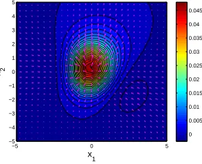
Figure 2– Exact surface displacement for the elliptic geometry and slip in the e2 direction considered in the

first example. In local coordinates the slip was picked to be g = C1

q

1−y˜12−( ˜y2/5)2e2, where

the constant C1 was adjusted in such a way that the total slip R_Γg be of norm 1. The e1 and e2

components ofu(x1, x2)are represented as a planar vector field using arrows, while thee3component

is sketched on the same graph using a color contour map.

x₁

x2

−5 0 5

−5 −4 −3 −2 −1 0 1 2 3 4 5 0 0.005 0.01 0.015 0.02 0.025 0.03 0.035 0.04 0.045

Figure 3– Exact surface displacements in the second example. The geometry of the fault is the same as in the first example, however the slip does not now have constant direction and is picked to be, in local

coordinates, g = C2(−2m3/2, m1/2,2m3/2) where m = 1−( ˜y1/5)2−y˜22 and the constant C2 was

adjusted in such a way that the total slip R

Γg be of norm 1.

3.

Approximate surface displacements fields

Solving equations (16-19) by integratingu= 1 2

R

ΓHgmight be expensive in number of operations, which is undesirable in applications where such a direct computation would have to be iterated a large number of times. We found a way to obtain a good approximate field u(x1, x2,0) based on asymptotics that just assume that (x1, x2) is some distance away from the fault Γ. Suppose that the fault Γ is centered at the point (a, b, c) where

c < 0. To obtain a simpler formula for the surface displacement u(x1, x2,0) we now assume that either the surface point (x1, x2) is far enough from (a, b) or|c|is large enough. Thus we may write

H(x1, x2,0, y1, y2, y3) =H(x1−y1, x2−y2,0,0,0, y3) =

H(x1−a, x2−b,0,0,0, c) +O(

1 (x2

as long as (y1, y2, y3) remains on the fault Γ. ¿From there,

u(x1, x2,0)'H(x1−a, x2−b,0,0,0, c) 1 2

Z

Γ

g(y1, y2, y3)dy (24)

Setting (t1, t2, t3) = 1₂R_Γg(y1, y2, y3)y, we obtain,

u(x1, x2,0)'H(x1−a, x2−b,0,0,0, c)(t1, t2, t3). (25)

The vectort:= (t1, t2, t3) can be interpreted as half the average slip on Γ times the area of Γ. We will call 2t the total slip on Γ.

We now proceed to demonstrate numerically the accuracy of approximation (25). We plot the relativeL2_error incurred in making the approximation (25) against depth, for three different geometries in Figure 4. The L2 error was computed on the surfacex3= 0 in a square [−10,10]×[−10,10]. In each case the fault was contained in the plane normal to the vector (1,0,1) and passing through the center (0,0, c), where|c|is the depth, which we varied form 2 to 20 in these numerical runs. Slip was set to occur in thee2direction. Total slip was computed in order to apply formula (25). The plus markers correspond to a square geometry with edges of length 2. In local coordinates ( ˜y1,y˜2) centered on the fault, the slip was picked to be

p

(1− |y˜1|)(1− |y˜2|). Local coordinates are now related to the original coordinates by

y=





s 0 s 0 1 0

−s 0 s



y˜+ 



0 0 c



, s=

1

√

2.

The star markers correspond to a circular geometry of radius 1. In local coordinates the slip was picked to be

p

1−y˜12−y˜22.

The circle markers correspond to an elliptic geometry. The equation of the ellipse was picked to be in local coordinates, ˜y12+ ( ˜y2/5)2= 1. In local coordinates the slip was picked to be

q

1−y˜12−( ˜y2/5)2.

The largest error is found for the most shallow faults, that is for|c|= 2, and ranges from 12% to 19%, depending on geometry. We sketched the exact and approximated fields in the elliptic geometry case in Figures 2 and 5. It appears that the exact and approximated profiles exhibit very similar profiles.

2 4 6 8 10 12 14 16 18 20 0

0.02 0.04 0.06 0.08 0.1 0.12 0.14 0.16 0.18 0.2

depth

relative L

2 error

Figure 4– The relative L2 _{error incurred by making the approximation (25) plotted against depth, for three}

different geometries. The L2 _{error was computed on the surface x}

3 = 0 in a square [−10,10]×

[−10,10]. In each case the fault was contained in the plane normal to the vector(1,0,1)and passing

through the center (0,0, c), where|c|is the depth. Slip was set to occur in thee2direction. The plus

markers correspond to a square geometry with edges of length 2. In local coordinates the slip was

picked to bep

(1− |y˜1|)(1− |y˜2|). The star markers correspond to a circular geometry with of radius

1. In local coordinates the slip was picked to be p1−y˜12−y˜22. The circle markers correspond to

an elliptic geometry. The equation of the ellipse is in local coordinates, y˜12+ ( ˜y2/5)2 = 1 In local

coordinates the slip was picked to be

q

1−y˜12−( ˜y2/5)2.

x

1

x2

−5 0 5

−5 −4 −3 −2 −1 0 1 2 3 4 5

−0.025 −0.02 −0.015 −0.01 −0.005 0 0.005 0.01 0.015 0.02

Figure 5– Approximate surface displacement for the elliptic geometry from Figure 4 at depth 2. The approxi-mation was obtained by applying formula (25). The computed exact field is sketched in Figure 2

4.

The fault inverse problem

4.1.

Statement of the inverse problem and parameters to be recovered

¿From the data u(x1, x2) = H(x1−a, x2−b,0,0,0, c)(t1, t2, t3) introduced in (25) our goal is to find (in a numerically robust fashion):

- the center of the fault Γ, (a, b, c)

- a tangent vector to Γ,t= (t1, t2, t3) giving the total slip on Γ as defined in the previous section

4.2.

Limitations

Due to the expression forH(x1−a, x2−b,0,0,0, c) it turns out thatu(x1, x2) is a function that depends on

nandt only throughs0, s1, s2, s3, s4 defined by

s0:=n1t1+n2t2 (26)

s1:=n2t3+n3t2 (27)

s2:=n1t3+n3t1 (28)

s3:=n1t2+n2t1 (29)

s4:=n1t1−n2t2 (30)

Proposition 4.1. Assume that n = (n1, n2, n3) and t = (t1, t2, t3) are two orthogonal vectors in space such

that |n| = 1 and |t| 6= 0. Given s0, s1, s2, s3, s4 defined in (26-30) exactly four different pairs (n, t) can be

reconstructed. If (˜n,˜t)is one reconstructed pair, the other three are (−n,˜ −˜t), (_|tt˜˜|,˜n|˜t|), and (−

˜

t

|˜t|,−n˜|˜t|).

proof:

The proof is given in [18].

5.

Proposed solution

Denote the coordinates of the surface displacementu1(x1, x2), u2(x1, x2),andu3(x1, x2). A calculation shows that

I1:=

Z Z

u1(x1, x2)dx1dx2=s2 (31)

I2:=

Z Z

u2(x1, x2)dx1dx2=s1 (32)

I3:=

Z Z

u3(x1, x2)dx1dx2=− 1 2

µ

λ+µs0 (33)

Note that the above integrals are not in L1 _{(meaning that they are not absolutely integrable). The integrand} can be expanded as A_ρ(2θ)+O(

1

ρ3), and it turns out that

R2π

0 A(θ)dθ = 0. The following six integrals will be needed

Ip,q := Z Z

up(x1, x2)uq(x1, x2)dx1dx2

=

Z Z

up(x1+a, x2+b)uq(x1+a, x2+b)dx1dx2

where 1≤p≤q≤3

integrals that depend linearly onb.

Jp,q:= Z Z

up(x1, x2)uq(x1, x2)x1dx1dx2

=

Z Z

up(x1+a, x2+b)uq(x1+a, x2+b)x1dx1dx2+aIp,q (34)

Kp,q:= Z Z

up(x1, x2)uq(x1, x2)x2dx1dx2

=

Z Z

up(x1+a, x2+b)uq(x1+a, x2+b)x2dx1dx2+bIp,q (35)

note that Jpq−aIpq andKpq−bIpq do not depend on aand b and are linear combinations of s_c2i, 0≤i≤4 whose coefficients depend only on the Lam´e constantsλandµ.

Equations (31-32) provides0, s1, s2. There remains to solve fors3, s4, a, b, c, which we proceed to do next. In some cases we will find expressions fors2

3, s24and quadratic equations forc2. The solution will have to be picked, depending on the case, within a set of 1,2, or 4 candidates. In practice making such a final pick is not costly, as we will retain the solution that leads to a reconstructed surface displacement field closest to the surface data. Remark The integrals Ip, Ip,q, Jp,q, Kp,q, can be computed in a closed form. Due to the complexity of the

expression for u(x1, x2) this can only be done using a symbolic calculation software. For brevity, we do not provide here the resulting expressions. Instead we indicate how those can be used to solve the fault inverse problem.

5.1.

The case

s

0

6

= 0

As n andt are perpendicular this is equivalent to the condition n3t3 6= 0. Physically, this means that the fault is not vertical and that the average slip is not horizontal.

5.1.1. Solving for the depth |c|

If

λ µ 6=

−1 +√10

3 , (36)

the depthc satisfies the equation

A1c4+A2c2+A3= 0 (37)

where we set

A1:= 1 2

(C3+C4) (I1,1−I2,2)2

s02(2C1−C2)2

+C4

I1,22

s02(C1−C6)2

,

A2:=−I1,1−I2,2−

C1(C3+C4) s22−s12(I1,1−I2,2)

s02(2C1−C2)2

−2C4

C1s1s2I1,2

s02(C1−C6)2

,

A3:= 2C1 s22+s12+ 2s02+ 1

2(C3−C4)s 2 0+

1

2(C3+C4)

C1 s22−s12 2

s02(2C1−C2)2

+C4

C12s12s22

s02(C1−C6)2

whereC2, C2, C4, C6 depend only onλandµ. It can be shown that due to (36)

2C1−C26= 0 (38)

C1−C66= 0 (39)

It can also be shown that I1,1+I2,2>0, therefore we can not haveA1=A2= 0: equation (37) is well posed.

Assume now that

λ µ =

−1 +√10

3 (40)

or equivalently 2C1−C2=C1−C6= 0. We find the following relations

(I1,1−I2,2)c2=C1(s22−s21) (41)

I1,2c2=C1s1s2 (42)

It follows from (40)thatC16= 0. Ifs1 =s2= 0,ccan be solved as indicated in case 5.1.4. Otherwisec can be solved by application of (41) or (42).

After solving forc we proceed to solve fors3 ands4

5.1.2. Case s06= 0 ands16= 0 The following formulas hold

s3=−−

(I1,3s1+I2,3s2)c2+ (−C1−C10−C11)s2s1s0

C1(s21+s22)

(43)

s4=−−c 2_I

2,3+ 1/2(−C1−C10−C11)s1s0+C1s3s2 1/2(−C1+C10−C11)s1

(44)

Our calculations show that (C1−C10+C11) =₃₂3_π, for all values ofλandµ. We can now apply section 4.2 to solve for the vectorsnandt.

5.1.3. Case s06= 0 ands26= 0

We can still use formula (43), and we use the following in place of (44)

s4=−−

c2_I

1,3+ 1/2(−C1−C10−C11)s2s0+C1s3s1 1/2(−C1+C10−C11)s2

(45)

5.1.4. Case s06= 0 ands1=s2= 0

In that case,c, s3, s4 can be solved for by using the following, assuming on the one hand (36),

c2= (4C1+C7)s 2 0

I3,3

(46)

s4=−(−I1,1+I2,2)c 2

(2C1−C2)s0 (47)

Assuming on the other hand that (40) holds we solve the equations

c2= (4C1+C7)s 2 0

I3,3

(49)

C4s23+ 1

2(C3+C4)s 2

4=−(4C1+ 1 2C3−

1 2C4)s

2

0+ 2c2I1,1 (50)

s2

3+s24=s20 (51)

where equations (50-51) form a non singular linear system ins2

3ands24. 5.1.5. Case s06= 0: solving for the horizontal position (a, b)

There remains one task: solving for the horizontal position (a, b). This is now straightforward by application of (34) and (35) for (p, q) equal to (1,1), or (2,2), or (3,3). This can be done because I1,1, I2,2, I3,3 to be simultaneously zero.

5.2.

Case

s

0

= 0

This case is very different. Note that asnandtare orthogonals0=−n3t3. Physically, this case corresponds to either vertical faults or horizontal total slips (or both). Note thats0=s1=s2= 0 if and only ifn3=t3= 0.

5.2.1. Case s0= 0 ands16= 0 ors26= 0 In that case, eithers2

1−s226= 0 ors1s26= 0. Ifs2

1−s226= 0 then, as in that caseI1,1−I2,26= 0

c2=C1

s2 2−s21

I1,1−I2,2

(52)

s3=−−(I1,3s1+I2,3s2)c 2

C1(s21+s22)

(53)

s4= −

(−I1,3s2+I2,3s1)c2

−1

2(−C1+C10−C11)(s22+s21)

(54)

where we recall that (C1−C10+C11) = ₃₂3_π, for all values ofλandµ. Ifs1s26= 0, asI1,26= 0,

c2₌ C1s1s2

I1,2

(55)

s3=−−

(I1,3s1+I2,3s2)c2

C1(s21+s22)

(56)

s4= −(−I1,3s2+I2,3s1)c 2

−12(−C1+C10−C11)(s22+s21)

(57)

There remains one task: solving for the horizontal position (a, b). This is done by application of (34) and (35) for (p, q) equal to (1,1), or (2,2), or (3,3).

5.2.2. Case s0= 0 ands1=s2= 0

We have in this casen3=t3= 0. Physically, the fault is vertical and the total slip is occurring in a horizontal direction. In this case, we begin by solving foraandbas we can show that

a=Jp,p Ip,p

forpbeing either 1, 2, or 3. If

λ µ 6=

−1 +√46

9 (58)

c is easily solved for too as

c=−C4 C13

K2,3

I1,1

,

whereC136= 0 due to (58). To solve fors3 ands4, we set

I20,3=

Z Z

x2>b

u2(x1, x2)u3(x1, x2)dx1dx2

It follows that

s23=

−4I0

2,3c2+A(2C16+C17)

C17−2C16 (59)

s24=−4

C16A−I20,3c2

C17−2C16

, (60)

whereA=2c 2

I1,1

C4 , and where it can be shown thatC17−2C16>0, for all positive values ofλandµ. If

λ µ =

−1 +√46

9 , (61)

the above solution is not valid asC13= 0. We then introduce

I10,3=

Z Z

x2>b

u1(x1, x2)u3(x1, x2)dx1dx2

J0

1,3=

Z Z

x2>b

u1(x1, x2)u3(x1, x2)(x1+a)dx1dx2

which are involved in the following equations

c2I1,1=C20s23 (62)

c2_I0

1,3=C21

s3s4

2 (63)

cJ10,3=C22

s3s4

2 (64)

where the constantsC20, C21, C22 are all non zero. Assume, thats3s46= 0. Thencis obtained by dividing (63) by (64), from where we can solve fors2

3 ands24.

6.

Numerical reconstruction

6.1.

Using formulas derived in the previous section

We now apply the reconstruction formulas derived in the previous section. To limit the number of runs presented in this paper and to facilitate comparison between these runs, we fixλ=µ= 1,a=−10,b= 10. We then consider different depthsc, different geometries (or rather fault orientation characterized byn) and total slips given byt. All considered cases are indicated in the first column of table 1. In each case we compute values for u(x1, x2), as defined in the previous section, where (x1, x2) is on a discrete grid of points defined by the square [−M, M]×[−M, M], M = 200, and the spacingh= 2. The integralsIp, Ip,q, Jp,q, Kp,q were evaluated

numerically from the discrete set of values for (x1, x2) by application of a simple order two quadrature rule combined with estimates of tails. We then applied formulas from section 5 to reconstruct (a, b, c), n, t. Solutions are reported in the second column of table 1. Note that in each case there are truly four equivalent solutions forn, t. We retained the one that makes for the easiest comparison to the data, for convenience.

We then found out that it is possible to sharpen our numerical solutions by applying a least square minimization technique. The minimization uses the discrete datau(x1, x2). The approximate solution provided in the second column of table 1 serves as a starting point for the minimization. The improved solution after minimization is borne out in the third column of table 1. Note that if minimization is started from a point too far away from the true values for(a, b, c), n, t, it is, in most cases, unsuccessful: this underscores the importance of inversion techniques developed in section 5.

The results obtained in the first case considered in table 1 may seem not as accurate when compared to results from other cases. In fact accuracy can be greatly improved in the first case for a smaller spacingh.

6.2.

Requirements on grids of data points

We inspected which are the smallest value forM and the largest value forh that will guarantee success of our numerical inversion for a given center (a, b, c) and anyn, twhere the discrete datau(x1, x2) is on the grid defined by the square [−M, M]×[−M, M], and the spacingh. It is in fact sufficient to carry out the inspection fora= 0, b= 0, c=−1 and to then infer all other cases by rescaling and horizontal translation. It was found that those smallest value forM and the largest value forhare (approximately)

Mmin=α|c|+|a|+|b|, hmax=5|c|

α (65)

where

2≤α≤4. (66)

a b c n1 n2 n3

t1 t2 t3

-10 10 -5 -11.4598 8.5814 -5.7761 -10.0242 9.9558 -5.0492 0.8660 0 0.5000 0.9144 0.0529 0.4014 0.8694 0.0154 0.4939 -1.0000 2.0000 1.7321 -0.8932 2.9833 1.6413 -1.0107 2.0236 1.7161 -10 10 -10 -12.9798 7.1005 -11.5655 -9.9819 9.9614 -10.0335 0.8660 0 0.5000 0.9157 0.0541 0.3982 0.8669 0.0100 0.4983 -1.0000 2.0000 1.7321 -0.8884 3.0055 1.6353 -1.0217 2.0025 1.7374 -10 10 -40 -16.7442 2.4340 -44.0588 -9.9501 9.9795 -40.0129 0.8660 0 0.5000 0.8997 0.0412 0.4345 0.8664 0.0041 0.4993 -1.0000 2.0000 1.7321 -0.9242 2.6311 1.6639 -1.0080 1.9955 1.7327 -10 10 -5 -10.0000 10.0030 -5.0000 -9.9994 10.0021 -4.9978 0.8660 0 0.5000 0.8657 - 0.0008 0.5005 0.8660 - 0.0006 0.5000 0 2.0000 0 0.0016 1.9993 0.0004 0.0009 1.9989 0.0007 -10 10 -10 -10.0229 10.0077 -10.0288 -10.0010 10.0030 -10.0018 0.8660 0 0.5000 0.8660 -0.0007 0.5001 0.8659 - 0.0002 0.5002 0 2.0000 0 0.0015 2.0061 0.0003 0.0004 2.0001 0.0004 -10 10 -40 -10.4012 9.8320 -40.1008 -9.9919 10.0081 -39.9959 0.8660 0 0.5000 0.8625 -0. 0.5061 0.8660 -0.0004 0.5001 0 2.0000 0 0.0017 2.0001 0.0077 0.0013 1.9988 -0.0006 -10 10 -5 -10.0001 10.0001 -5.0118 -9.9999 10.0000 -4.9999 0.7071 0.7071 0 0.7071 0.7071 0.0000 0.7071 0.7071 -0.0000 0 0 2.0000 -0.0000 0.0000 2.0044 -0.0000 0.0000 2.0000 -10 10 -10 -10.0015 10.0015 -10.0435 -10.0000 9.9999 -10.0000 0.7071 0.7071 0 0.7071 0.7071 0 0.7071 0.7071 0.0000 0 0 2.0000 -0.0000 0.0000 2.0088 -0.0000 0.0000 2.0000 -10 10 -40 -10.0509 10.0509 -40.2883 -10.0000 9.9996 -39.9993 0.7071 0.7071 0 0.7071 0.7071 -0 0.7071 0.7071 0.0000 0 0 2.0000 -0.0038 0.0038 2.0291 -0.0000 0.0000 2.0000 -10 10 -5 -10.0024 10.0000 -4.8745 -10.0009 10.0084 -4.9986 0.7071 0.7071 0 0.7071 0.7071 -0.0000 0.7071 0.7071 0.0015 2.0000 -2.0000 0 2.0144 -2.0144 -0.0064 2.0030 -2.0029 0.0043 -10 10 -10 -10.0082 10.0002 -9.5237 -9.9991 10.0002 -9.9956 0.7071 0.7071 0 0.7071 0.7071 -0.0026 0.7071 0.7072 0.0005 2.0000 -2.0000 0 1.9072 -1.9072 0.0000 2.0002 -1.9999 -0.0009 -10 10 -40 -9.0590 10.0016 -56.8499 -9.9894 10.0500 -40.0016 0.7071 0.7071 0 -0.9099 -0.4149 -0.0003 0.7063 0.7080 -0.0007 2.0000 -2.0000 0 1.6529 -3.6253 -0.0031 2.0036 -1.9988 0.0011

Table 1– Reconstruction of faults defined by (a, b, c), n, t. First column indicates specific values in each case.

In all cases λ = µ = 1, and values for u(x1, x2) are computed for (x1, x2) on a discrete grid of

points defined by the square [−M, M]×[−M, M], M = 200, and the spacing h= 2. Second column

7.

Detecting active faults from GPS observations

The aim of this section is to account for the sensitivity of measuring apparatus and for the observation grid stepsize, and to understand how those may affect detection of active faults. In an attempt to model real life situations we choose a threshold under which surface displacements cannot be measured. Moreover, we allow ourselves to use only a limited number of measurement points, on a fixed grid, independently of the geometry and the size of the fault, and location of the center of the fault.

7.1.

Sensitivity and indicative points

By definition, at fixed sensitivityS, a point (x1, x2) on the grid of measurement points is said to be indicative if

|u(x1, x2)| ≥S,

where u(x1, x2) is the surface displacement generated by a given slip on the fault Γ. Next, at fixed sensitivity

S, we define the indicative setI to be

I :={(x1, x2)∈R2; |u(x1, x2)| ≥S}.

7.2.

Fault recovery at fixed observation sensitivity

We now seek to evaluate how the sensitivity of observations affect our inversion techniques. We know from the previous subsection that sensitivity is related to the stepsize of the grid.

We apply the reconstruction formulas derived in section 5, while taking into account a sensitivity thresholdS. We repeat some of the runs from table 1 at sensitivity levelS = 2·10−5 _{for all cases with one exception: this} high sensitivity level led to failure of the recovery method for the case c = −40 n = (0.8660,0,0.5000), t = (−1.0000,2.0000,1.7321). We made a second run in that case with the sensitivity S = 10−5 _{which led to a} successful recovery. All outputs of successful runs appear in table 2. In each case we plotted the region of [−M, M]×[−M, M], M = 200 comprised of indicative points (points where|u| ≥ S). These plots appear in Figure 6.

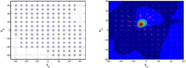
Finally we present a reconstruction calculation in case of scarce data,M =Mmin,h=hmax, (see formula (65)),

at sensitivityS= 4·10−5_{. The values fornand tfor this run are indicated in Table 3. With those values for}

a b c n1 n2 n3

t1 t2 t3

-10 10 -5 -9.3626 10.4380 -5.4635 -10.0431 10.0359 -5.1183 0.8660 0 0.5000 0.8067 -0.0622 0.5877 0.8600 -0.0130 0.5102 -1.0000 2.0000 1.7321 -1.5165 1.8331 2.2752 -1.0468 2.0037 1.8154 -10 10 -10 -3.8306 12.8072 -9.6300 -9.9316 10.0195 -9.9248 0.8660 0 0.5000 0.8077 0.1184 0.5776 0.8650 0.0023 0.5018 -1.0000 2.0000 1.7321 -1.9958 0.6539 2.6566 -0.9971 1.9754 1.7096 -10 10 -40 28.0423 29.8760 -32.0114 -9.9138 9.9576 -39.9913 0.8660 0 0.5000 -0.7673 -0.2060 -0.6073 0.8669 0.0107 0.4984 -1.0000 2.0000 1.7321 2.4998 0.0825 -3.1867 -1.0240 1.9724 1.7390 -10 10 -5 -10.0000 10.0000 -4.3542 -9.9999 10.0003 -5.0001 0.7071 0.7071 0 0.7071 0.7071 0.0000 0.7071 0.7071 0.0000 0 0 2.0000 -0.0000 -0.0000 1.7412 -0.0000 -0.0000 2.0001 -10 10 -10 -10.0000 10.0000 -7.9563 -10.0000 10.0000 -10.0000 0.7071 0.7071 0 0.7071 0.7071 0.0000 0.7071 0.7071 0.0000 0 0 2.0000 0.0000 -0.0000 1.5903 -0.0000 -0.0000 2.0000 -10 10 -40 -10.1213 10.1213 -19.3468 -10.0003 10.0005 -39.9993 0.7071 0.7071 0 -0.7071 -0.7071 0.0000 0.7071 0.7071 -0.0000 0 0 2.0000 0.0012 -0.0012 -0.9467 0.0001 -0.0001 2.0000

Table 2– Reconstruction of faults defined by (a, b, c), n, t, at sensitivity S = 2·10−5_{, except in the third case}

where sensitivity had to be lowered to S= 10−5_{. First column indicates specific values in each case.}

In all cases λ = µ = 1, and values for u(x1, x2) are computed for (x1, x2) on a discrete grid of

points defined by the square [−M, M]×[−M, M], M = 200, and the spacing h= 2. Second column

indicates reconstruction after application of formulas derived in section 5. Third column contains sharper results obtained by applying a least square minimization technique with results from column two as initial values.

a b c

n1 n2 n3

t1 t2 t3

-10 10 -10 -17.7778 -10.7818 -33.9972 -10.0020 10.0038 -10.0030 0.8660 0 0.5000 0.9722 0.2300 0.0447 0.8659 -0.0005 0.5001 -1.0000 2.0000 1.7321 -4.9816 20.7632 1.5182 -0.9998 2.0003 1.7329

Table 3– Example of reconstruction from very scarce data. Sensitivity was set atS= 4·10−5_{, data is sampled}

−200 −150 −100 −50 0 50 100 150 200 −200

−150 −100 −50 0 50 100 150 200

−200 −150 −100 −50 0 50 100 150 200

−200 −150 −100 −50 0 50 100 150 200

−200 −150 −100 −50 0 50 100 150 200

−200 −150 −100 −50 0 50 100 150 200

−200 −150 −100 −50 0 50 100 150 200

−200 −150 −100 −50 0 50 100 150 200

−200 −150 −100 −50 0 50 100 150 200

−200 −150 −100 −50 0 50 100 150 200

−200 −150 −100 −50 0 50 100 150 200

−200 −150 −100 −50 0 50 100 150 200

−60 −40 −20 0 20 40 60 −60

−40 −20 0 20 40 60

x

1

x2

x

1

x2

−60 −40 −20 0 20 40 60

−60 −40 −20 0 20 40 60

Figure 7– Above: the set of data points used for the inversion procedure whose output is provided in table 3.

Appendix

Instead of giving formulas for each entry of the matrixH, it is advantageous to write out formulas for the coordinatesH t wheretis the vector (t1, t2, t3). We only present in this appendix formulas atx3= 0: the idea is to give a feel for the different terms involved. The complete formula forx3<0 is best left within a computer code.

It proves convenient to introduce polar surface coordinates.

7.3.

If

(

x

1

−

y

1

)

2

+ (

x

2

−

y

2

)

2

= 0

The three coordinates ofH tare then, respectively,

0 0

−µ(n1t1+n2t2) + 6 (λ+µ)n3t3 4πy32 (λ+µ)

7.4.

If

(

x

1

−

y

1

)

2

+ (

x

2

−

y

2

)

2

>

0

We set

ρ=p(x1−y1)2+ (x2−y2)2

d=

q

ρ2_+y2 3

c= x1−y1 ρ

s= x2−y2 ρ .

The first coordinate ofH tis the ratio of

αn1t1+βn2t2+γn3t3+δ(n1t2+n2t1) +(n1t3+n3t1) +ζ(n2t3+n3t2) (67)

to

(λ+µ)π ρ3d5 (68)

where, setting

A= y3dρ4+ 5/2y34+ 2y33dρ2+y36+y35dµ ,

α, β, γ, δ, γ, , ζ are given by,

α

c =−A 4c

2

−3

+

3/2λ c2+µ

ρ6−1/2µ 15c2−11

y32ρ4,

β

c =A 4c

2₋₃ −

3/2λ c2−1

ρ6+ 3/2µ 5c2−4

γ

c = 3/2 (λ+µ)y3

2_ρ4_,

δ

s =−A 4c

2

−1

+

3/2λ c2+ 1/2µ

ρ6−1/2µ 15c2−4

y32ρ4,

=−3/2ρ5_y

3c2(λ+µ),

ζ =−3/2 (λ+µ)csy3ρ5.

The second coordinate of H tis also in form of the ratio of (67) to (68), where this time α, β, γ, δ, γ, , ζ are given by

α

s =−A 4c

2

−1

+

3/2λ c2ρ6−3/2 5c2−1

µ y32ρ4,

β

s =A 4c

2₋₁

+

3/2λ+µ−3/2λ c2

ρ6+ 1/2µ −4 + 15c2

y32ρ4,

γ

s = 3/2 (λ+µ)y3

2_ρ4_,

δ

c =A 4c

2

−3

+

3/2λ+ 1/2µ−3/2λ c2

ρ6_{+ 1/2µ 15c}2₋₁₁

y32ρ4,

=−3/2 (λ+µ)csy3ρ5,

ζ = 3/2ρ5y3 c2−1(λ+µ).

Setting,

B= 1/2dρ5+dy32ρ3+ 1/2y35+ 1/2y34dρµ ,

the third coordinate ofH tis also in form of the ratio of (67) to (68), where this timeα, β, γ, δ, γ, , ζ are given by,

α=−B −1 + 2c2

+

−3µ c2−3/2λ c2+µ

y3ρ5−1/2µ 5c2−3y33ρ3,

β=B −1 + 2c2

+

−2µ+ 3/2λ c2−3/2λ+ 3µ c2

γ=−3/2 (λ+µ)y33ρ3,

δ

sc = ((−3/2λ−3µ)y3−dµ)ρ

5₊

−5/2µ y33−2dµ y32ρ3+ −dµ y34−µ y35ρ,

c = 3/2 (λ+µ)y3

2_ρ4_,

ζ

s = 3/2 (λ+µ)y3

2_ρ4_.

Remark: Denote (u1, u2, u3) the coordinates of Ht, whose expressions were given above. The following sym-metry properties hold:

u1(s, c, n1, n2, t1, t2) =u2(c, s, n2, n1, t2, t1),

u3(s, c, n1, n2, t1, t2) =u3(c, s, n2, n1, t2, t1).

These symmetry properties can be easily verified using thats2_+c2_{= 1. Physically, they express that the first} and the second coordinate play the same role for the displacement vectorHt, on the surfacex3= 0.

Acknowledgments

This is joint work with I. R. Ionescu. Partial support for this work was provided by NSF grant DMS 0707421.

References

[1] M. Abramowitz and I. Stegun, eds. (1992), Handbook of Mathematical Functions with Formulas, Graphs, and Mathematical Tables, Dover, New York.

[2] Dieterich, J.H.A model for the nucleation of earthquake slip, in Earthquake source mechanics, Geophys. Monogr. Ser., vol. 37, edited by S. Das, J. Boatwright, and C.H. Scholz, AGU, Washington, D. C. (1986), pp. 37-47.

[3] W.L. Elsworth and G.C. Beroza,Seismic evidence for an earthquake nucleation phase, Science, vol. 268 (1995), 851–855. [4] Y. Iio, Slow initial phase of the P-wave velocity pulse generated by microearthquakes, Geophys. Res. Lett., vol. 19(5) (1992)

pp. 477-480.

[5] I. R. Ionescu, D. Volkov, An inverse problem for the recovery of active faults from surface observations, Inverse Problems 22 (2006) 2103-2121.

[6] I. R. Ionescu, D. Volkov, Earth surface effects on active faults: an eigenvalue asymptotic analysis, Journal of Computational and Applied Mathematics archive Volume 220 , Issue 1-2 (October 2008).

[7] I. R. Ionescu, D. Volkov, Detecting tangential dislocations on planar faults from traction free surface observations, submitted to Inverse Problems.

[8] V. Kostoglodov, S. K. Singh, J.A. Santiago, S.I. Franco, K.M. Larson, A.R. Lowry and R. Bilham, A large silent earthquake in the Guerrero seismic gap, Mexico,Geophys. Res. Lett., Vol. 30 (15), (2003), doi:10.1029/2003GL017219

[9] A.R. Lowry, K.M. Larson, V. Kostoglodov and O. Sanchez, The fault slip budget in Guerrero, southern Mexico,Geophysical Journal, International, Vol. 200, (2005), pp. 1-15

[10] P. A. Martin, L. P¨aiv¨arinta, S. Rempel, A normal crack in an elastic half-space with stress-free surface. (English summary, Math. Methods Appl. Sci. 16 (1993), no. 8, 563–579.

[11] R. D. Mindlin, Force at a point in the interior of a semi infinite solid, Physics Vol. 7, 1936, p 195-202.

[12] M. Ohnaka, Y. Kuwakara and K. Yamamoto, Constitutive relations between dynamic physical parameters near a tip of the propagation slip during stick-slip shear failure,Tectonophysics,144(1987), 109-125.

[13] V.Z. Parton, P.I. Perlin, Integral Equations in Elasticity, Moscow, Mir Publisher, 1982. MR 509209 (80a:73001)

[14] T. Sagiya and S. Ozawa, Anomalous transient and silent earthquakes along the Nankai Trough subduction zones, Seismol. Res. Lett., vol. 73 (2), (2002), 234-235

[16] J. A. Steketee, On Volterra’s dislocations in a semi infinite elastic medium, Canadian Journal of Physics, 36, 1958, p 192-205. [17] E. P. Stephan, A boundary integral equation method for three dimensional crack problems in elasticity, Mathematical Methods

in the Applied Sciences, 1986, Volume 8-4, 609-623.