F. Coquel, M. Gutnic, P. Helluy, F. Lagouti`ere, C. Rohde, N. Seguin, Editors
CURRENT IDENTIFICATION IN VACUUM CIRCUIT BREAKERS
AS A LEAST SQUARES PROBLEM
∗Luca Ghezzi
1and Francesca Rapetti
2Abstract. In this work, a magnetostatic inverse problem is solved, in order to reconstruct the elec-tric current distribution inside high voltage, vacuum circuit breakers from measurements of the outside magnetic field. The (rectangular) final algebraic linear system is solved in the least square sense, by involving a regularized singular value decomposition of the system matrix. An approximated distri-bution of the electric current is thus returned, without the theoretical problem which is encountered with optical methods of matching light to temperature and finally to current density. The feasibility is justified from the computational point of view as the (industrial) goal is to evaluate whether, or to what extent in terms of accuracy, a given experimental set-up (number and noise level of sensors) is adequate to work as a “magnetic camera” for a given circuit breaker.
R´esum´e. Dans cet article, on r´esout un probl`eme inverse magn´etostatique pour d´eterminer la dis-tribution du courant ´electrique dans le vide d’un disjoncteur `a haute tension `a partir des mesures du champ magn´etique ext´erieur. Le syst`eme alg´ebrique (rectangulaire) final est r´esolu au sens des moin-dres carr´es en faisant appel `a une d´ecomposition en valeurs singuli`eres regularis´ee de la matrice du syst`eme. On obtient ainsi une approximation de la distribution du courant ´electrique sans le probl`eme th´eorique propre des m´ethodes optiques qui est celui de relier la lumi`ere `a la temp´erature et donc `a la densit´e du courant. La faisabilit´e est justifi´ee d’un point de vue num´erique car le but (industriel) est d’´evaluer si, ou `a quelle pr´ecision, un dispositif exp´erimental donn´e (nombre et seuil limite de bruit des senseurs) peut travailler comme une “cam´era magn´etique” pour un certain disjoncteur.
Introduction
Circuit breakers are protection devices which are inserted into electric networks in order to clear faults such as short circuits and overloads. Under faulty and possibly dangerous conditions, circuit breakers are operated in such a way to break the electric current flow by opening two contacting conductors, thus interrupting the electric continuity of the line. The technology adopted in circuit breakers, along with the size, depends on their rating, ranging from small devices that protect an individual household appliance up to large switchgear designed to protect high voltage circuits or power generators.
Whenever a current is interrupted, an electric arc is generated. This arc must be contained, cooled, and extinguished in a controlled way, so that the gap between the contacts can again withstand the voltage in the circuit. The medium in which the arc forms depends on the circuit breaker and may be vacuum, air, insulating gas (SF6,CO2), or even oil in old times. A common aspect is the crucial role played by plasma dynamics with
∗This project was supported by the grantMortar Elements for Industrial Devices (MEID)of the programProjets Exploratoires
PluridisciplinaireS (PEPS)in the themeMathematics in Industry (MI)funded by the CNRS-INSMI Institute. 1 ABB S.p.A., Via dell’Industria 18, 20010 Vittuone, Italy
2 Laboratoire J.A. Dieudonn´e, Universit´e de Nice Sophia-Antipolis, Parc Valrose, 06108 Nice c´edex 02, France c
EDP Sciences, SMAI 2012
reference to the final interruption outcome, which makes the arc the core technological issue in circuit breaker engineering; see [3]. The knowledge of electric current distribution in space and time, during an interruption process, helps understanding the complex physical behavior of the electric arc and allows technicians to evaluate the effect of design choices.
Standard experimental techniques for arc diagnostic are of optical nature, including imaging by means of CCD cameras or fiber optics. Despite being well assessed and appreciated, optical methods are deemed invasive and to some extent perturbative of the real physical conditions, since observations screens of different materials are produced, or holes for hosting fibers are drilled in the sidewalls of otherwise opaque circuit breakers. The preparation of the experimental setup is also time consuming and not easy, especially in the case of vacuum circuit breakers, owing to the need for preserving gastightness and preventing the surrounding atmosphere from penetrating inside the breaker. To prevent from saturation of the filming device, optical methods require suitable and non trivial filtering techniques, which may strongly affect the reliability of the collected data; see [7]. The translation of an observed light pattern into a temperature pattern and, finally, into an electric current density pattern is an issue itself, whose complexity is increased by the progressive blindening of the optical tool, produced by the soot and debris released during arcing.
An alternative experimental method is the reconstruction of the current distribution from measurements of the magnetic field. An inverse problem needs to be solved, allowing the determination of the causes, i.e., electric currents inside the circuit breaker, starting from the effects, i.e., the magnetic field outside the circuit breaker. In this work, we analyze from the numerical point of view the magnetic inverse problem to solve for the current reconstruction in the circuit breaker chamber. In the linear algebra framework, we are concerned with the least squares solution of a system of equations where the system matrix is generally rectangular (more unknowns than equations or viceversa) and frequently rank deficient. We note that the numerical solution of linear least-squares problems is a key computational task in science and engineering. Effective algorithms have been developed for the linear least-squares problems in which the underlying matrices have full rank and are well-conditioned. However, there are few efficient and robust approaches to solving the linear least-squares problem in which the underlying matrices are rank-deficient and sparse. The method to solve the considered circuit breaker problem is based on a classical Single Value Decomposition (SVD) of the system matrix [5] combined with a particular Smith normal form (SMF) algorithm [8, 9] for the divergence-free constraint on the current density.
1.
Continuous direct problem description
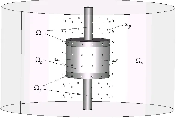
The current identification method is applied to a Vacuum Circuit Breaker (VCB). A simplified geometry of a typical VCB is shown in Fig. 1. The VCB is constituted by two copper terminals, occupying domains Ω1
and Ω2. The shape of each of the two conductors is approximated by the union of circular disc and a slender
cylinder, the latter being the connection of the VCB to the rest of the electric network. When the breaker is in closed position, the two discs contact one against the other. As soon as the contacts are opened, a cylindrical gap is formed, occupying the domain Ωp. Such a gap hosts the plasma phase, where electric current density has to be identified.
We denote by Ωc:= Ω1∪Ωp∪Ω2 the conductive or potentially conductive portion of the problem at hand,
including into this denomination also those region of Ωp characterized by a low electrical conductivity. The surrounding domain Ωais occupied by external air, and has to be considered as insulating, since electric current has no way to leave Ωc. Finally we introduce the domain Ω := Ωc∪Ωa. We may assume, with no loss of generality as regards the technical application, that both Ωc and Ω are simply connected.
In absence of (linear or nonlinear) ferromagnetic inclusions and charge accumulation, the direct problem consists in finding the magnetic field H which is related in Ω to the conduction current densityJ and to the magnetic flux densityBby
Figure 1. Geometry of a VCB.
where µ = µ0 since we consider “vacuum” circuit breakers. We remark that even in presence of para- or
dia-magnetic media in the breaker, the assumption µ=µ0 is still considered at the engineering level since the
highest errors are related to measurements. Problem (1) is closed by suitable boundary conditions related to the total currentI flowing through the VCB. Indeed, let∂Ω1
c (resp.,∂Ω2c) be the “in” (resp., “out”) terminal, i.e., the portion of the boundary∂Ωc of the conducting domain Ωc where electric currentI1=−I (resp.,I2= +I)
enters into (resp., exits from) Ωc. We may always assume, up to swapping the names of domains, that ∂Ω1
c (resp.,∂Ω2
c) be a portion of the boundary∂Ω1 (resp.,∂Ω2) of Ω1(resp., Ω2). LetA1(resp.,A2) be the surface
area of∂Ω1
c (resp.,∂Ω
2
c). Let∂Ω
0
c =∂Ωc\(∂Ω
1
c∪∂Ω
2
c) be the lateral skin of Ωc, that is, the interface between Ωcand Ωa. Since the latter is insulant, no cross flow of electric current is possible andJis tangent to∂Ω0
c, thus
Z
∂Ωi c
J·n=Ii, i∈ {0,1,2}, (2)
whereI0:= 0.
2.
Discrete inverse problem description
In order to state the discrete inverse problem, we firstly introduce T, a conforming discretization of the domain ¯Ω, consisting in oriented cells, that are simplices in the present case. LetSn be the set ofn-simplices of the complex T =∪3
n=0Sn. We termN =S0,E=S1,F =S2 andC=S3 the node, edge, face and cell sets,
respectively, of the complex T. Then|N |, |E|, |F| and|C| are the number of nodes, of edges, of faces and of cells, respectively. Additionally, let T1,T2, Tp, andTc be the sub-complexes ofT discretizing Ω1, Ω2, Ωp, and
Ωc, respectively. Union and intersection relations, such asT1∪Tp∪T2=Tc, are naturally inherited by analogous
relations holding in the exact, continuous frame. Finally, let|Np|,|Ep|,|Fp|and|Cp|be the number of nodes, of edges, of faces and of cells ofTp, respectively. Analogous definitions are assumed for the other sub-complexes.
Experimental or synthetic measures of the magnetic field intensityH are available in a collection{xp}|P|p=1 of
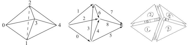
Figure 2. A simple mesh of two outwardly oriented simplices. The associated data structure includes the set of nodesN ={0,1,2,3,4}, the set of (internally) oriented edgesE ={ {0,1},
{0,2}, {0,3}, {1,2}, {1,3}, {1,4}, {2,3}, {2,4}, {3,4} }, the set of oriented facets F =
{ {0,1,2}, {0,1,3}, {0,2,3}, {1,2,3}, {1,2,4}, {1,3,4}, {2,3,4} } and the set of oriented tetrahedra T ={ {0,1,2,3}, {1,2,3,4} }. In this case, D is a 2×7 integer matrix with first line equal to (−1,1,−1,1,0,0,0) and second line (0,0,0,−1,1,−1,1).
each probe senses the whole magnetic field vector; the latter condition may always be obtained, albeit in a somewhat approximated way, by locating three directional sensors very close together, in a neighborhood of the same point, and aligned along three independent directions. We denote by|P|the number of sensors available, so that 3|P|is the number of measures. We thus introduce a vectorh of size 3|P| to collect the vectorsHp, that are the measures of the field H associated to the points xp. We denotes by j the vector containing the degrees of freedom ofJover the mesh T, that are the values of the electric density fluxes across the|F|mesh faces. The inverse discrete algebraic counterpart of problem (1) reads: find jsuch that
Dj=0 and Lj=h, (3)
whereDis the face-to-volume incidence matrix andLa linear discrete analogue of the Biot-Savart operator [1]. Note that, in typical industrial applications,|F| ≫3|P|.
The first equation in problem (3) represents the discrete form of the divergence free constraint on the current density J. The involved face-to-volume incidence matrixD is a|C| by|F|integer matrix with entries
Dcf ∈ {0,1,−1}, where|C|(resp. |F|) is the number of cells (resp. faces) in the meshT. In detail,Dcf = 0 iff is not a face of the cellc. Otherwise,Dcf = +1 (resp. −1) iff is a face ofcand its internal (for example counter-clockwise) orientation agrees (resp., disagrees) with the face orientation induced by the outward orientation of
c onf; see Fig. 2.
Letn:= dim kerDbe the dimension of the null space ofDandN ∈R|F |×nbe a matrix whose columns form a basis for kerD. SinceDNz=0,∀z∈R|F |, the expression
j=Nz (4)
originates a generic divergence free current density distribution. Plugging (4) into (3), one gets the linear system to solve, namely findz∈R|F |such that
LNz=h. (5)
Despite the divergence free constraint allows eliminating a number of unknowns, the algebraic system (5) on the free unknowns typically remains underdetermined. The matrix N can be computed relying on the Smith normal form ofD as described in the next section.
3.
Integer QR factorization with column pivoting to construct
N
(SVD) of A or on theQR factorization of A with column pivoting, a method proposed by Golub in the mid-sixties [5]. The second method is much cheaper than the SVD and consists in using a column pivoting strategy to determine a permutation matrixP such thatAP =QRwithQ∈Rn×n satisfyingQ⊤Q=I
n and the upper triangular matrix Ris partitioned as
R=
R11 R12
0 R22
where R11∈Rr×rand R22 is small in norm. Let us assumeσ1≥σ2 ≥...≥σn ≥0, where σi are the singular values of A. Mathematically, in terms of singular values, we say that Ahas rank r if and only if σr >0 and
σr+1= 0. However, computationally, we may haveσr+1 not exactly equal to zero butσr+1=O(ν), whereν is
the machine precision. Ifσr≫σr+1, we say thatAhas numerical rankr. Equivalently, if, say,||R22||2=O(ν),
it can be proved thatσr+1≤ ||R22||2. Thus we conclude that the original matrixAis guaranteed to haveat most
numerical rankr, that is, rankrup to the precisionν. TheQRfactorization ofAP, whereP is a permutation matrix chosen to yield a “small”R22, is referred to as the Rank-Revealing QR (RRQR) factorization ofA.
With both SVD and RRQR decompositions, the matrixAcan be factorized as
A=UΣV⊤, (6)
where U ∈Rn×n and V ∈Rm×m are orthogonal matrices and Σ∈Rn×m. Being orthogonal, the rows as well the columns ofUandV spanRnandRm, respectively. All of the non-zero entries of Σ are on the main diagonal and we suppose that these entries are ordered in such a way that the firstr are non-null, while the remaining
p−rare null, withp:= min{m, n}. This is always possible by means of a suitable permutation of the rows and columns ofA which will be memorized in the matricesU andV. In short, the following structure holds:
Σ =
d1 . . . 0 0 . . . 0
..
. . .. ... ... ... ... 0 . . . dr 0 . . . 0 0 . . . 0 0 . . . 0
..
. . .. ... ... ... ... 0 . . . 0 0 . . . 0
. (7)
The nullspace ofA is contained inV:
The nullspace (or kernel) of matrixA is a vector subspace ofRm of those vectorsxsuch thatAx=0. Owing to the factorization (6), withU invertible, the condition forxto be in the nullspace of Amay be rewritten as
ΣV⊤x=0. (8)
Let us expand explicitly the above product and write
y:= ΣV⊤x=
d1v⊤1x
.. .
drv⊤ rx 0 .. . 0
∈Rn. (9)
The condition that the newly introduced vector y must be null implies div⊤
i x = 0, i ∈ {1, . . . , r}. Since
di 6= 0,i∈ {1, . . . , r}, by hypothesis, this implies v⊤i x= 0,i∈ {1, . . . , r}. In short,x⊥<v1, . . . ,vr>, i.e.,x
A U Σ VT
=
r
n n r
r
n
m im(A)
ker(A)
m m m
n n
Figure 3. Visual sketch of the factorization (6), revealing the nullspace kerA(spanned by the
rows in the gray part of matrixV⊤) and the range imA(spanned by the columns in the gray part of matrixU); the main diagonal of each matrix is shown as a guide to visualize the matrix size; the bold part of the main diagonal of Σ contains the only non-null entries of such a matrix.
x must lie in the orthogonal complement of<v1, . . . ,vr>in Rm, which is the subspace spanned by the last m−rcolumns ofV. We thus have that the lastm−rcolumns ofV span the nullspace ofA.
The range of A is contained inU:
The range ofAis the subspace ofRn generated by those vectors of the formAxwithx∈Rm. We remind that
Ax=Uy. Thei-th component of the generic element of the range reads
(Ax)i= n
X
j=1
Uijyj= r
X
j=1
Uijyj+ n
X
j=r+1
Uij·0 = r
X
j=1
Uijyj, (10)
where the last passage holds because the lastn−rentries ofyare zero by (9). Therefore, the lastn−rcolumns of U do not contribute to give Ax, while others do. This means that the last n−r columns of U span the orthogonal complement of the range ofAin Rn. We thus have that the firstrcolumns of U span the range of
A. A visual sketch of the decomposition is shown in Fig.3.
We now particularize the RRQR to treat integer matrices with entries in{0,1,−1}and get aQRfactorization such thatQandRcontains entries which are still in{0,1,−1}, further detailing the presentation given in [8]. In the considered circuit breaker, the integer matrix is the volume-to-face incidence matrixDwhich appears in the divergence-free constraint on the global current densityj. To this purpose, we introduce suitable terminology.
A unimodular matrixM is a square integer matrix with determinant±1. Equivalently, it is an integer matrix that is invertible over the integers and its inverse is again a unimodular matrix. Note that permutation matrices are unimodular as well as matrices obtained by taking products of unimodular matrices are still unimodular.
A totally unimodular (TU) matrix is a matrix for which every square non-singular submatrix is unimodular. A TU matrix is not necessarily square. Moreover, from its definition it follows that any TU matrix has only entries in the set {0,+1,−1}. We note that the incidence matrixD is TU, as every column of D contains at most two-non zero entries (since an internal face is shared by two cells and a boundary face only by one cell) and its entries are 0,+1,−1. Moreover, it cannot happen that two non-zero entries in a column ofD have the same sign since all tetrahedra in a automatically generated mesh have an outward orientation, thus, as in Fig. 2, if a facef is shared by two cells, the orientation off agrees with that induced on it by one cell but disagrees with that induced on it by the other cell. These conditions together are sufficient forD to be a TU matrix.
For a TU matrixA∈ M(ℓ, q), we compute a unimodular matrixQand a permutation matrixP such that
R=QAP
op1 transformation of a vector v= (ǫi, ǫj)⊤ into the vector ˜v= (1,0)⊤. This can be done by multiplyingv on the left by the 2×2 matrix
Qel i,j =
ǫi 0
−ǫi ǫj
!
thanks to the fact that, in our case, ǫ2
i = 1.
op2 permutation of a vector components, i.e., transformation of a vector v = (ǫi, ǫj)⊤ into the vector ˜
v= (ǫj, ǫi)⊤. This can be done by multiplyingv on the left by the 2×2 matrix
Pel i,j=
0 1
1 0
!
Then, we can define
Q= Πlef tQi,j , P= ΠrightPi,j
where the notation Πlef t (resp., Πright) indicates that the matrices Qi,j (resp., Pi,j) have to be multiplied successively on the left (resp., on the right) and
Qi,j(s, r) =
I(s, r) s6=i , j r6=i , j Qel
i,j(1,1) s=i r=i
Qel
i,j(1,2) s=i r=j
Qel
i,j(2,1) s=j r=i
Qel
i,j(2,2) s=j r=j
The matrix Pi,j is similarly defined (just replace Qeli,j with Pi,jel in the previous definition). We remark that (Pel
i,j)−1=Pi,jel due to the fact thatPi,jel is a permutation matrix ((Pi,jel)2=I2). The inverse ofQeli,j is given by
(Qel i,j)−1=
ǫi 0
ǫj ǫj
!
.
Then (Qi,j)−1 is defined as before just replacingQel
i,j with (Qeli,j)−1 and finally we have
Q−1= ΠrightQ−1
i,j , P−
1= Πlef tP−1
i,j.
Now we describe the adopted procedure1to build upQ andP for a given TU matrixA.
function [Q,R,P]=smith(A) Initialization step:
Q=Iℓ , P =Iq per each column j with 1≤j≤min{ℓ, q} do
(1) local initialization step : k= 0, i1= 0, i2= 0
1The two functions “smith” and “nullspace” are originally written (in pseudo-language) by the authors, they do not exist
(2) loop on the rowsi withj≤i≤ℓ to define
Vj={i|j≤i≤ℓ , A(i, j)6= 0} , k= card (Vj)
i1= min(Vj) , i2= min(Vj\ {i1})
(3) in case k = 0 : let Pj,z be the matrix that permutes the jth column of A with the zth one. The zth column is chosen to be the first column, counted out starting from the last one, for which it exists a row index ssuch that A(s, z)6= 0. If the index z does not exist, then stop and R=A, otherwise do
P ←− P Pj,z
A ←− APj,z
and go back to step 2.
(4) in case k 6= 0 but A(j, j) = 0 we apply a sort of partial pivot strategy : let Qj,i1 be the matrix that
permutes the jth row with thei1th one (as explained in op2) and do
Q ←− Qj,i1Q
A ←− Qj,i1A
i1 ←− j
and go to step 5.
(5) in case k6= 0 andA(j, j)6= 0, then :
if k= 1, do j←− j+ 1 and restart the procedure from step 1.; if k≥2, let Qel
i1,i2 be the matrix that transforms the vector (A(i1, j), A(i2, j))
⊤ into the vector (1,0)⊤
(as explained in op1) and Qi1,i2 the associated matrix, then do
Q ←− Qi1,i2Q
A ←− Qi1,i2A
and go back to step 1.
At the end of the procedure, the matrixAhas been replaced byR, an upper triangular one. The null space of a matrix is not affected by elementary row operations. This makes it possible to usesmith(D) to compute
N. Starting fromD we thus use the procedure given below, sinceD has entries in the set{−1,0,1}.
function[N] =nullspace(D) Initialization step:
r= size(D,1), s= size(D,2), p=min(r, s),
(1) Use elementary row operations to putD in reduced row echelon form. To this purpose run [Q1, R1, P1]= smith (D)to getR1 upper triangular and run[Q2, R⊤, P2]= smith (R1⊤) to getR diagonal;
(2) determinerk, the rank ofR, by checking how many diagonal entries ofR are different from zero; (3) setn=s−rk, wherenis the dimension of the nullspace of D, and initializeN with
N = zeros(s, n).
variables. Thus, for each free variable xi, choose the vector for which xi = 1 and the remaining free variables are zero. Then, the matrix N of sizes×n is composed as follows
N(j, i) =−R(j, rk+i), i= 1, n, j= 1, r,
N(rk+i, i) = 1, i= 1, n
(5) apply back the two vector basis changes computed at steps (1) and (2), thus
N ←− P1Q2⊤N.
4.
The regularized LS problem
Problem (5) is solved in the least squares sense by relying on suitable factorizations of the matrixLN with real entries, as described at the beginning of section 3. If we setA=LN, x=zand b=h, the least squares (LS) form of the system of equations (5) reads
find z∈R|F |−|C| s.t. ||LNz−h||2
2= min
y∈R|F |−|C|||LNy−h||
2
2. (11)
The numerical solution of (11) lies at the heart of many computational problems arising in scientific, engineering and economic disciplines. Efficient algorithms are available when the system matrix has full rank and is well-conditioned. However, when the matrix is ill-conditioned or rank-deficient, numerical solution of (11) often requires some variant of rank-revealing QR factorization (RRQR) or singular value decomposition (SVD). Unfortunately, the column pivoting required in the RRQR strategy does not always work for a generic real matrix. This is a very interesting but delicate subject that goes beyond the scope of the present work. Note that the modified version presented in section 3 for TU matrices does not suffer from this inconvenient. To stay on the safe side with real matrices, we solve problem (5) by using the SVD of LN. Indeed, we know that the solution to (5) is not unique as n≤m. Thus, the minimum-norm solution
z= arg min
y∈RnkLNy−hk
2
2 (12)
is sought for, that is given by j = (LN)†h, where (LN)† is the pseudo-inverse ofLN computed by its SVD, defined as
(LN)† =VΣ†U⊤. (13)
4.1.
Error norms
We start with a reference current density distributionjrefto identify. then we superimpose Gaussian noise to
exact synthetic datahref=Ljref, and we measure the amount of noise by the signal to noise ratior(or better, by
its reciprocal, which is more suited for the present purposes). Currentsjrec,r are identified by solving the inverse problem with noisy data (jrec,0is the solution to the inverse problem without noise). The original referencejref
and reconstructed jrec,r current distributions are compared and the errorjerr,r =jrec,r−jref is evaluated. The
magnetic fieldhrec,r =Ljrec,r, relevant to the reconstructed currents, is computed and compared withhref, and
the error herr,r=hrec,r−hrefis also evaluated.
Two merit indicators are defined, namely the relative errors on currents and magnetic fields, in the 2-norm:
ǫj:=
kjerr,rk2 kjrefk2
, ǫh:=
kherr,rk2 khrefk2
. (14)
Since the goal of the method is to reconstruct currents, the most appropriate and ultimate error evaluator is a measure of the entity ofjerr,r, i.e., ǫj. The error on magnetic fields and thenǫh is a side-product which can be
0 50 100 150 200 250 300 350 400 450 500 10−8
10−7 10−6 10−5 10−4 10−3 10−2 10−1 100
Singular spectrum
i
s i
/ s
max
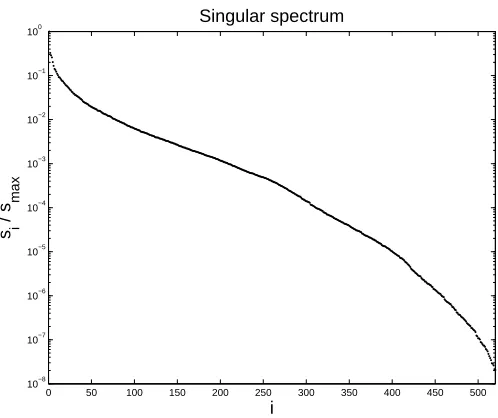
Figure 4. Singular value spectrum for a typical VCB case (fine approximating mesh and fine
sensor array).
4.2.
Tikhonov regularization and TSVD
A difficulty with inverse source magnetic problems is that they are notoriously ill-posed. If we consider noise as a perturbation on the magnetic field measures, the corresponding perturbation propagated to the currents is bounded by
kjrec,r−jrec,0k2 kjrec,0k2
≤κ2
khexp,r−hexp,0k2 khexp,0k2
∼κ2r, (15)
where
κ2:= smax
sr
(16)
is the condition number (in the 2-norm) of LN, that generalizes the analogous concept for standard linear systems with non singular matrices. If κ2 ≫ 1, it is possible (and virtually certain) that the unstabilized
solution (12) is completely unreliable and useless. This is due to the large nullspace ofLN and the consequent impossibility to block the back propagation of noise. By (16), small, non-null singular values, either intrinsic to theLN operator or of numerical error origin, yield a high condition numberκ2 (in fact, they result into large
reciprocals in Σ†). Therefore they need to be filtered out in order not to possibly enhance noisy components of the measures.
A typical singular value spectrum of the problem at hand is shown in Fig. 4. The singular values are observed to decay gradually toward zero and do not show an obvious jump between zero and nonzero singular values. The condition number κ2 remains finite, though very large. It is not infrequent that the maximum singular
value be tenths of orders of magnitude bigger than the smallest non-null singular value. After [2] and [6], we refer to an inverse problem with these features as adiscrete ill-posed problem. A typical regularization technique for such a class of problems isTikhonov regularization [2], [6], arising from finding a minimizer
z= arg min
y∈R|F |−|C| kLNy−hk
2 2+α
2kyk2 2
(17)
Figure 5. Discrete approximation of the VCB: fine mesh (left) and coarse mesh (right).
Other regularization techniques may be adopted and we use a synthetic representation for all of the most used ones. Let
(LN)♯:=V FΣ†UT (18)
be theregularized inverse [6], that is, the regularized counterpart of (13), whereF∈End(Rn) is a suitable filter matrix. For our needs it is sufficient to consider diagonal filter matrices of the form Fij =fiδij, where
fi:=
sβi
sβi +αβ
if si
smax > δ
0 (otherwise).
(19)
Whenδ= 0 andβ= 2, one finds Tikhonov regularization with the parameterα≪smax. It is immediately seen
that the effect of Tikhonov regularization is to reduce the contribution of progressively smaller singular values (si ≪α), for whichfi →0 and (FΣ†)ii =fi/si ∼si/α2 →0. When δ= 0 andβ = 1, one finds the damped SVD, similar to Tikhonov regularization but with a milder decay rate for small singular values. Whenα= 0 andβ >0, one finds thetruncated singular value decomposition (TSVD), such that all singular values below a toleranceδ≪smaxare forced to zero.
The regularized solution, replacing (12), reads
j=N(LN)♯h. (20)
It is important to notice that regularizing is not for free. As a matter of fact, with regularization schemes of the kind (19), the singular spectrum of the governing operator is altered, so that a practically unattainable precision is sacrificed, to some extent, for the sake of stability. As a consequence, the regularization scheme introduces a theoretical lower bound to the attainable accuracy.
5.
Numerical examples
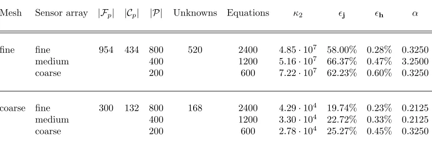
The current reconstruction method is tested numerically, according to what detailed hereafter. A summary of all results is reported in Table 1, where the model space (mesh,|Fp|,|Cp|) and data space (sensor array,|P|) are described, along with the resulting dimensions (number of unknowns and of equations) and conditioning (κ2) of the governing linear operator. For each case, the errors on currents (ǫj) and magnetic field (ǫh) are
We first consider a simple case characterized by |N |= 626 vertices, |E|= 3300 edges,|F|= 4914 faces and
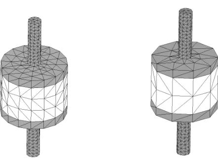
|C|= 2239 cells. This mesh will be termed fine; see Fig. 5 (left). The inverse problem is reduced to the plasma domain only, by means of a suitable condensation technique [3], such that the metal conductorsT1 andT2 are
condensed onto their interface surfaces with the plasma domainTp. The resulting, reduced, condensed problem has now only |Fp| = 954 faces and |Fc| = 434 cells. The divergence free constraint is introduced through the nullspace spanning matrix N, which has dimensions 954 by 520. Therefore, 434 additional equations, corresponding to the tetrahedra inTp, are introduced by the divergence free constraint, lowering the number of unknowns from 954 to 520.
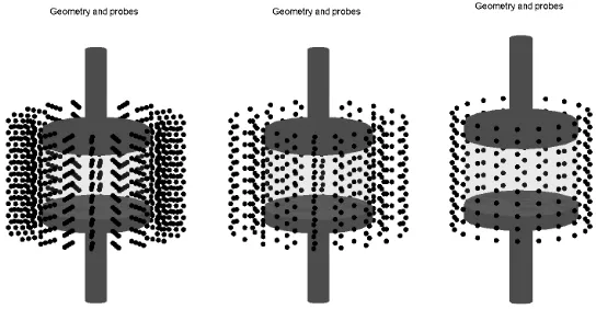
We use an array of 800 sensors (3|P|= 2400), located according to a cylindrical array with 4 layers of 10 circles with 20 probes along the circumference; see Fig. 6, left. This arrangement yields an over-determined system of equations, with matrixLN which is 2400 by 520. The singular spectrum of LN is shown in Fig. 4. The minimal and maximal singular values are found to besmin= 1.0997·10−5andsmax= 533.85, respectively.
The resulting condition number is thus κ2 = 4.85·107, a value that leaves no hope to approach a noisy case
without regularization.
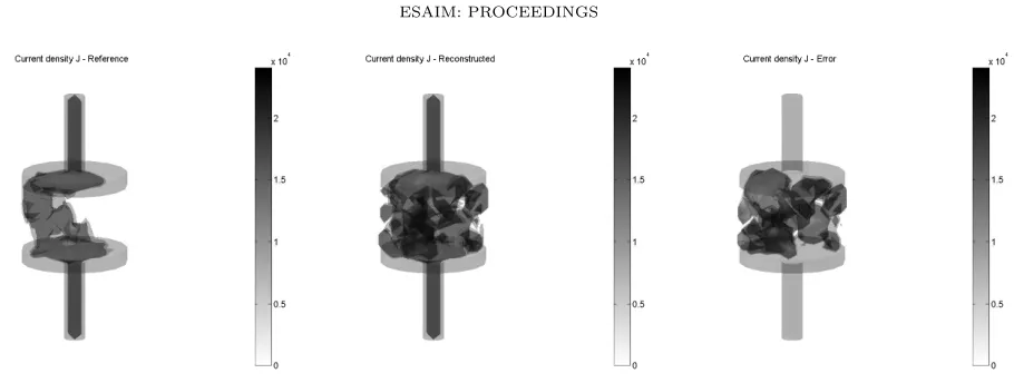
First, a noiseless condition is resolved. The procedure works very effectively, and no regularization is needed. A relative error on currentsǫj= 0.67% is found. The magnetic fields are practically exact, with a relative error ǫh= 8·10−11. Fig. 7 shows the current density field: reference (left), reconstructed (center) and error (right).
Two ISO-magnitude surfaces are shown, partially transparent and relevant to 20% and 24% of the maximal value of current density magnitude (note that the error is not in scale with the other two). The visual effect is that of a practically perfect reconstruction of the current density field.
Then, a noisy condition with signal-to-noise ratio (SNR) 1/1% is approached. As expected, the superimposed noise on the measurements has a disruptive effect on the ill-conditioning of the LN operator. We try to heal the inverse problem solution by means of Tikhonov regularization, obtaining the trends shown in Fig. 8, where in the left picture the relative errors on currents (bold line) and magnetic fields (thin line) are drawn Vs. theα
penalty factor (adimensionalized by the greatest singular value). Asαis increased, a steep descent is observed in the error on currents, from hyperbolic values down to ǫj = 58.00%. The right picture is a parametric plot
originated by the two relative errors, takingαas a parameter, and shows that the best compromise is found in the bend of the typical L shaped curve. Consequently, the error on magnetic fields is still low, and precisely
ǫh = 0.28%. Unfortunately, the error on currents, even in the best case, is useless for engineering purposes,
and some finer approach is needed. Fig. 9 shows the current density field, under the same assumptions already discussed in the exact case.
We tested the method also with the sensor arrays shown in Fig. 6 (center and right) and characterized by, respectively, only 2 and 1 layers, instead of 4. The good quality of the exact case solution is preserved, as well
Figure 6. Array of sensors located around the VCB under test: fine (left), medium (center),
Figure 7. Current density field in a noiseless case, with a fine mesh and fine sensor array: reference (left), reconstructed (center) and error (right).
as the trends and values observed in the regularization of the noisy case. Similar results (not reported) are obtained by means of the TSVD regularization scheme.
Since the problem with inverse identification is its ill-conditioning, and since the condition number increases with the size of the problem, the current reconstruction method is also tested on a coarser mesh, characterized by |N | = 497 vertices, |E| = 2567 edges, |F| = 3786 faces and |C| = 1715 cells. This mesh will be termed coarse; see Fig. 5 (right). When reduced to the plasma domain only, the resulting, condensed problem has now only|Fp|= 300 faces and|Cp|= 132 cells. The divergence free constraint is introduced through the nullspace spanning matrix N, which has dimensions 300 by 168. Therefore, 132 additional equations, corresponding to the tetrahedra inTp, are introduced by the divergence free constraint, lowering the number of unknowns from 300 to 168.
The fine sensor array is still used; see Fig. 6, left. This arrangement yields an over-determined system of equations, with matrix LN which is 2400 by 168. The minimal and maximal singular values are found to be
10−5
10−4
10−3
10−2
10−1
100
10−3
10−2
10−1
100
101
102
Error vs. Tikhonov regularization α parameter
α / s
max
εj
and
εh
10−3
10−2
10−1
100
10−1
100
101
102
α = 0.2125 − α / smax = 0.00039805
Error vs. Tikhonov regularization (parametric plot)
εh εj
Figure 8. Tikhonov regularization in a noisy case (SNR=1/1%), with a fine mesh and fine
sensor array. Left picture: error on currents (bold line) and on magnetic field (thin line) Vs. α
Figure 9. Current density field in a noisy case (SNR=1/1%), with a fine mesh and fine sensor array: reference (left), reconstructed (center) and error (right).
Figure 10. Current density field in a noisy case (SNR=1/1%), with a coarse mesh and fine
sensor array: reference (left), reconstructed (center) and error (right).
smin = 7.2727·10−3 andsmax = 311.79, respectively. The resulting condition number is thus κ2= 4.29·104,
which is three orders of magnitude lower than in the fine mesh case.
The noisy condition with signal-to-noise ratio (SNR) 1/1% is solved. A similar exploration method is used to get the optimalαpenalty factor. Correspondingly, the error on currents has decreased down toǫj= 19.74%,
and the error on magnetic fields is always low, and preciselyǫh= 0.23%. Fig. 10 shows the current density field,
under the same assumptions already discussed. Although the error on currents is better but still useless for engineering purposes, this test shows a clear trend (expected from the theory of inverse problems) and suggests trying to adopt a multi-scale approach, starting with a coarse mesh and later refining the result with finer grids. Well assessed regularization techniques exist, based on Tikhonov method, in order to penalize strong deviations from a former, coarser estimate of the solution; see, e.g., [6]. This idea is not developed in the present study.
6.
Concluding remarks
Mesh Sensor array |Fp| |Cp| |P| Unknowns Equations κ2 ǫj ǫh α
fine fine 954 434 800 520 2400 4.85·107 58.00% 0.28% 0.3250
medium 400 1200 5.16·107 66.37% 0.47% 3.2500
coarse 200 600 7.22·107 62.23% 0.60% 0.3250
coarse fine 300 132 800 168 2400 4.29·104 19.74% 0.23% 0.2125
medium 400 1200 3.30·104 22.72% 0.33% 0.2125
coarse 200 600 2.78·104 25.27% 0.45% 0.3250
Table 1. Summary of numerical results: all cases with signal-to-noise ratio = 1/1% (noiseless
case are solved practically exactly).
Electric, Pennsylvania Breaker, Siemens, Toshiba, Koncar HVS, BHEL, CGL, Square D (Schneider Electric). We have led a preliminary (simple and numerical) study of the current identification in vacuum circuit breakers. From the analyzes carried out it follows that it is numerically feasible to reconstruct the electric currents in the plasma phase inside a high voltage, vacuum circuit breaker by inverting magnetic field data. The presented results can however be improved by relying on other more sophisticated regularization techniques as well as by analyzing other ways to construct the Biot-Savart-like operator L, involving for example suitable (Whitney) elements [1] for the current and the magnetic field.
References
[1] A. Bossavit,Computational Electromagnetism. Academic Press, New York (1998).
[2] R.C. Aster, B. Borchers, C.H. Thurber,Parameter Estimation and Inverse Problems, Elsevier Academic Press (2005). [3] L. Ghezzi, A. Balestrero,Modeling and Simulation of Low Voltage Arcs, Ph.D. Dissertation, Technische Universiteit Delft
(2010).
[4] L. Ghezzi, D. Piva, L. Di Rienzo,Current Density Reconstruction in Vacuum Circuit Breakers by Inverting Magnetic Field Data, IEEE Transactions on Magnetics, under review.
[5] G.H. Golub, C.F. Van Loan,Matrix computations, The Johns Hopkins University Press, Maryland (1985).
[6] P.C. Hansen.Rank-Deficient and Discrete Ill-Posed Problems, Numerical Aspects of Linear Inversion.Society for Industrial and Applied Mathematics (1998).
[7] J.W. McBride, A. Balestrero, L. Ghezzi, G. Tribulato, K.J. Cross. Optical fiber imaging for high speed plasma motion diagnostics: Applied to low voltage circuit breakers,AIP Rev. Sci. Instr., 81(5) (2010).
[8] F. Rapetti, F. Dubois, A. Bossavit,Discrete vector potentials for non-simply connected three-dimensional domains, SIAM J. on Numerical Analysis, 41(4) (2003), pp. 1505-1527.