Integrated AC transmission network expansion and reactive power planning

© Shiraz University

INTEGRATED AC TRANSMISSION NETWORK EXPANSION

AND REACTIVE POWER PLANNING

*

M. RAHMANI AND M. RASHIDINEJAD

**

Dept of Electrical Engineering, Shahid Bahonar University of Kerman, Kerman, I. R. of Iran Email: [email protected]

Abstract– An integrated technique for solving transmission network expansion planning considering the allocation of reactive power sources using an AC model is presented in this paper. Embedding reactive power management in TNEP is a challenging task since AC load flow may not converge in absence of proper reactive power allocation. Usually transmission expansion planning and reactive power planning are considered as two distinct problems, but in this paper both problems are investigated concurrently. These two problems can be integrated because there is an inherent interaction between transmission line capacity and reactive power sources. In power systems, transferring reactive power may engage line capacity which requires more new transmission lines, while allocating reactive power sources close to the load centers may prevent the addition of new transmission lines. On the other hand, if reactive power sources are not included, real power losses will increase considerably and thereby reduce transmission line capacities. The main objective of this study is to show that both active and reactive power planning can be handled simultaneously. This non-convex combinatorial optimization problem is solved here using a real genetic algorithm (RGA). Significant results through case studies of two test systems show the advantages of the proposed integrated network planning.

Keywords– Transmission expansion planning, real genetic algorithm, reactive power planning, AC optimal power flow, VAr sources

1. INTRODUCTION

Transmission network expansion planning (TNEP) and reactive power planning (RPP) are crucial issues, especially in deregulated power systems. In the environment of a restructured electricity industry, open access to transmission systems introduces new challenges to market participants. As electricity consumption grows, new transmission lines are needed to provide alternative paths for power transfer from generators to load centers to assure continuous supply. On the other hand, reactive power sources are desired to support available transfer capability (ATC), power factor correction, loss reduction and voltage profile improvement. The voltage collapse phenomenon and other instability problems can be related to the system’s inability to meet reactive power demands. When AC model is used for TNEP, it makes sense to consider reactive power allocation simultaneously, because lack of reactive power support can lead to either 1) no convergence of the load flow program or 2) unrealistic results due to Q absorption by generators due to line charging VARs or 3) unacceptably low voltages in the system [1].

Despite the implicit interdependence of RPP and TNEP, due to the complexity of merging these two problems, each problem is solved separately. In this study a new methodology is proposed to solve these complicated problems concurrently. In the traditional approach, transmission network planning problem is

solved using simplified models. The transportation model, the hybrid model, the linear disjunctive model, and the DC model [2], among others, are used in this first stage, and the problem is solved through classical optimization techniques [3–6] as well as evolutionary algorithms such as simulated annealing [7], genetic algorithms [8-10], tabu search [11], GRASP [12], ant colony [13] and also hybrid heuristic algorithms [14]. Then, in a subsequent stage, the obtained expansion network is reinforced with new lines and reactive power sources [15-20] to satisfy all requirements of a real AC network. The problem of dealing with real power losses, reactive power demands, incorporating FACTS devices into the system, voltage stability and other operational requirements are other issues that may arise when working with the DC model in transmission planning. Since active and reactive power planning are dependent on each other, these approaches may not achieve the optimal solution. The interdependence of transmission lines and reactive power sources can be addressed as follows:

1. Reactive power demands: these are an inherent part of any load center and must be procured either locally, through reactive sources, or produced by generators and transferred through transmission lines.

2. Real power losses: these also occur in any transmission network and reduce transmission capacity effectively. Transmission line capacity can be increased by line reinforcement or reactive power support.

In this study a comprehensive model for integrated transmission expansion and reactive power planning using the AC model is employed.

Integrated transmission expansion and reactive power planning is a very complex mixed integer nonlinear programming problem and becomes more complicated, especially when the size of the transmission network increases. The use of metaheuristic approaches seems to be necessary for solving such a non-convex problem. In this study a real genetic algorithm (RGA) [14, 21] is used to solve the planning problem, since GA is suitable for multi-objective optimization problems resulting in good solutions while maintaining low computational efforts. RGA is used to handle discrete variables in a major problem and a nonlinear constrained optimization for fitness function evaluation is solved in a minor problem. The objective function of the minor problem is minimum active power losses associated with the minimum value of reactive power sources.

This paper is organized as follows: section 2 gives an overview of the TNEP-RPP problem, section 3 presents mathematical modeling of combined AC TNEP-RPP; in section 4, the optimization process is described; in section 5, a modified Garver system is used as an illustrative example and for further analysis of the proposed method; in section 6, a modified IEEE 24-bus system is employed as another practical case study. Conclusions are made in section 7.

2. OVERVIEW OF TNEP-RPP PROBLEM

sources from step 2, the RPP problem is solved to find the location and minimum capacities of the VAr-plants needed for feasible system operation. In [22] a constructive heuristic algorithm (CHA) is proposed to allocate transmission lines in an iterative manner, while the reactive sources are allocated prior to lines allocation at weak buses using an index obtained by the Lagrange multiplier of the reactive power balances in each bus. The main characteristics of [1, 21-22] are that all of them solve the TNEP-RPP in several steps where it seems difficult to obtain the optimum solutions by these methods.

3. MATHEMATICAL MODELING

A mathematical model for the TNEP and RPP problem can be formulated in equations (1–11):

0

min _{v =c n}T ₍₁₎

1 Loss

min ( , )

v

=

K P D F

_e

+

q x

(2) s.t.

( , , )

θ

−

_G

+

_D

=

0

P U

n

P

P

(3)

( , , )

θ

−

_G

+

_D

− =

Q U

n

Q

Q

q 0

(4)

G

≤

G

≤

G

P

P

P

(5)

G G

G

≤

≤

Q

Q

Q

(6)

≤ ≤

q q q

(7)

≤ ≤

U U U (8)

0 from 0

(N N S+ ) ≤(N N S+ ) (9)

0 to 0

(N N S+ ) ≤(N N S+ ) (10)

0

≤ ≤

n n

(11)

n

and

u

are integer and

θ

is unbounded

where:

c

and n represent the costs vector of the prospective transmission lines and the prospective transmission lines, respectively.

N

and _N0_{are diagonal matrices containing prospective and the existing} circuits, respectively.

K

_e is the cost of energy, D is the system operating time,

P

_Loss is the total real power loss, F( , )q x is the cost function of VAr sources and q is the MVAr size of the VAr sources vector. x is the binary vector that indicates whether or not to install reactive power sources at load buses.

0

v

is the investment due to the addition of new circuits to the networks;

v

₁ is the total cost of active power losses and VAr sources. n is the vector containing the maximum number of prospective transmission lines.

θ

is the phase angle vector.

P

_G and

Q

_G are the existing real and reactive power generation vectors.

D

P

and

Q

_D are the real and reactive power demand vectors;

U

is the voltage magnitude vector;

P

G,QG

are the apparent power flow vectors (MVA) in the branches in both terminals and their limits. The objective function Eq. (1) considers only the expansion costs of transmission lines, while the objective function Eq. (2) considers the minimum cost of power losses associated with the costs of VAr sources that can be installed. Equations (3) and (4) represent the conventional equations of AC power flow considering n, the number of circuits (lines and transformers), and q, the size of VAr sources, as variables. The limits for real and reactive power in the generators are represented by Eq. (5) and Eq. (6), respectively; for VAr sources by Eq. (7) and for the voltage magnitudes by Eq. (8). The limits (MVA) of the flows are represented by Eq. (9) and Eq. (10). The constraints in the capacities of the added circuits are represented by Eq.(11). The costs of the VAr sources can be defined as follows:

0 1

( , )

(

)

l

k k k k

k

F

c

c q x

∈

=

∑

+

Ω

q x

(12)

where

Ω

_l represents the set of all load buses, and

c

_0k and

c

_1k are the installation cost and unit cost of the VAr source at bus

k

.

q

_kis the MVAr size of VAr source at bus

k

.

x

_k is a binary variable that indicates whether or not to install reactive power source at bus

k

. The active power losses can be calculated by the following equation:

2 2

[

2

cos(

)] g

Loss i j i j i j ij

ij

P

U

U

U U

θ θ

∈Ω

=

∑

+

−

−

(13)

Where: Ω is the set of all transmission lines,

U

_{i and}

θ

_{i are the magnitude and angle of voltage at bus} i.

ij

g is the conductance of the line between buses i _and

j

. The P U( , , )

θ

n and Q U( , , )

θ

n in equations (3) and (4) are basic AC power flow elements and they are given various papers [21-23]. The integer variable n, the number of circuits added in branch

ij

, and the binary variable x, and connection or disconnection of VAr sources to a load bus are the most important decision variables, and a feasible operation solution of the electric power system depends on these values. The remaining variables only represent the operating state of a feasible solution. For a feasible investment proposal, defined through specified values of n and x, one can have several feasible operation states.

4. OPTIMIZATION PROCESS

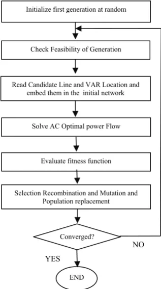
Different steps to find the optimum solution for TNEP-RPP are described as follows:

a) Initialization of the first generation

Each individual is chosen in a random fashion, while the data of an individual are the number and location of new lines as well as the location of VAr sources at load buses. The individual is a solution proposal for the planning problem, or better yet, is the topology made up of all transmission lines and reactive power sources added to the system corresponding to an investment proposal. In TNEP-RPP individuals are represented by a vector size. Each vector is constructed as the number of new transmission lines that are proposed to be added to respective branches and those load buses that VAr sources might be allocated to [25]. The value of each new transmission line can vary between zero and the maximum number of lines. For reactive power sources, two choices are possible: whether to install reactive power sources or not. Thus in the codification shown in Fig. 2, branch 2–6 has two new lines; branch 3–5 has one new line and bus 4 is a candidate for reactive power sources.

b) Feasibility checking

In TNEP-RPP, which is NP-hard [1], computational requirements of an optimization solver blow out with the dimensionality of the problem. Hence, the solution of TEP problem within the framework of optimization generally requires a reduction in search space. In order to reduce the search space of the problem each individual is checked in terms of costs; those individuals whose investments are too high will be pruned

1-2 1-4 3-5 2-6 4-6 . . . 2 4

0 0 1 2 1 . . . 0 1

Branches reactive power sources

Initialize first generation at random

Check Feasibility of Generation

Read Candidate Line and VAR Location and embed them in the initial network

Solve AC Optimal power Flow

END Evaluate fitness function

Selection Recombination and Mutation and Population replacement

Converged?

NO YES

Fig. 1. Flowchart of the TNEP considering reactive power allocation using RGA

out. However, it should be noted that setting a low threshold for pruning individuals may cause the algorithm to lose the optimum solution or even the high quality solutions.

c) Setting up the network

Read out the data of each individual, consisting of the number and location of new lines and the location of VAr sources and construct the new network. However, some individuals may create an unconnected network. The unconnected network may consist of several subsystems. A subsystem is referred to as a set of buses and transmission lines which are not connected to other subsystems. In this case special care should be taken into account when solving the AC optimal power flow. A common task for this difficulty is to solve an AC-OPF for each subsystem, and then sum up the objective function of each AC-OPF as the overall objective function.

d) Solving AC-OPF

For each individual, solve a particular AC optimal power flow with real and reactive power sources as optimization objectives. In this step the following problem is solved:

1 Loss

min ( )

v

=

K P D f

e

+

q

(14)

st.

( , )

θ

−

_G

+

_D

=

0

P U

P

P

(15)

( , )

θ

−

_G

+

_D

− =

Q U

Q

Q

q 0

(16)

G

≤

G

≤

G

P

P

P

(17)

G G

G

≤

≤

Q

Q

Q

(18)

≤ ≤

q q q

(19)

≤ ≤

U U U (20)

from

≤

S

S

(21)

to

≤

S

S

(22)

θ

is unbounded.

When new lines are embedded in the initial network, there is no need to separate the existing lines from new lines; i.e. all lines are existing lines. Also, since new VAr sources are included in the system, the binary variable vector x, connection or disconnection of a VAr source to a load bus is unnecessary in this formulation. There is no integer variable in this formulation, so we just need to solve an AC OPF. This problem can be solved using any nonlinear programming software.

e) Fitness function evaluation

behavior of the aforementioned objectives. However, other techniques could be implemented to calculate fitness. The fitness of a solution is assessed against the degree of membership of a specific solution to a given membership function [26, 27], where higher membership values imply a better solution, as described in Fig. 3.

Fig. 3. A typical membership function

Membership values can be represented by Eq. (23) which lies between 0 and 1, where

h f X

_i

( ( ))

is a strictly monotonically decreasing function that can be either linear or nonlinear.

min

min max

max 1 if ( )

( ) ( ( )) if ( ) 0 if ( )

i

i i

f i i i i

i i

f X f

X h f X f f X f

f X f

μ

⎧ < ⎫

⎪ ⎪

⎪ ⎪

=_⎨ ≤ ≤ _⎬

⎪ _> ⎪

⎪ ⎪

⎩ ⎭

(23)

Since the main objective of a TNEP-RPP is to minimize the costs of new transmission lines and VAr sources such that all constraints must be satisfied, fitness evaluation can be based upon Eq. (24).

1 1( )0 2 2( ) ( (1 3 3 ) 4( ) 5( ))

fitness w=

μ

v +w

μ

v + w

μ

dU +

μ

dG +

μ

dS (24)

Where all terms of the fitness function are fuzzy numbers with the appropriate membership function.

1

,

2

w w

and

w

₃ are tuning weights which can be selected by a decision satisfying Eq. (25).

1 2 3

1

w w

+

+

w

=

(25)

0

v

is the total cost of new lines and

v

₁ is the total cost of VAr sources.

d

_U

,

d

_G and

d

_Sare the sum of constraints deviations from voltage limits, power generation limits and branch flow limits, respectively. These Parameters are obtained after solving the AC OPF discussed in the last subsection. The range of fitness function is between 0 and 1, such that when the fitness value equals one it means that the costs of new transmission lines as well as the costs of VAr plants are zero (

v

₀

=

0

,

v

₁

=

0

). It can also be said that the deviations from the AC OPF constraints are zero, which means that all decision variables are inside their limits (

d

_U

=

0;

d

_G

=

0;

d

_S

=

0

).

f) Real genetic operators

When OPF is solved for the entire individuals and the fitness values of each is figured out, the selection, recombination, and mutation operators of RGA are implemented in order to construct a new generation of individuals. These operators are not described in this paper. A detailed discussion about RGA operators is given in [14, 21, 23].

5. CASE STUDIES

Unfortunately, we were unable to compare the results of this paper with other papers since the TNEP problem and RPP are usually solved and reported separately. There are only a few works that consider both TNEP and RPP jointly. However, the case studies proposed in [1], [21- 23] were found insufficient for implementing in this paper. In [1] the case studies and the proposed strategy, the possibility of installing the new transmission lines in the system is not considered; it only considers the reinforcement of the existing transmission lines. In [21- 23] the authors modified the original data provided in [1, 29] in which the generators and maximum flow capacity of transmission lines are augmented; modifying the tests systems will not provide the planner with the importance of implementing of TNEP-RPP and the necessary reinforcement of the system when compared with DC TNEP reported in many papers. To implement RGA for optimum TNEP-RPP, a population of 100 individuals is used, while recombination and mutation rates are 76 % and 3 %, respectively. The selection process would be terminated when there is no new individual in the population. Since in GA new generation may consist of previous individuals, a pool of all individuals is constructed to speed up the process. To calculate the fitness function for repetitive individuals we do not carry out all the calculations and simply pull out the fitness values from the pool. All calculations are carried out for the new individuals and, finally, their data and fitness values are inserted into the pool. One of the important parameters in this paper is the cost of energy

K

_e. This parameter depends on the average cost of energy in a year. For example, the values for peak wholesale and average retail electricity prices in the United States for the year 2006 are given in [29]. However, the updated prices can be obtained from [30]. This paper does not obtain the updated cost of energy since the costs of transmission lines are not updated. Instead these parameters are adjusted in a manner to be comparable with the transmission lines cost. In this paper, since the cost of energy is provided annually, the cost of transmission lines must also be provided annually. It is usually assumed that a line built today will be operative for several years [31]. To have an estimate of the annual transmission line costs the capital recovery factor might be calculated as(1+i)n_{/[ (1+i)}n _{-1], where}

i

_{is the discount rate and}

n

_{is the} number of years [31]. This paper assumes that the provided costs of energy for case studies in [2, 28] are annual.

a) Garver 6-bus system

For the illustrative examples, the Garver 6-bus system is used. This system has 6 buses and 15 branch candidates with a total demand of 760 MW and 190 MVAr, and a maximum of 5 lines can be added to each branch. Since the real transmission lines have shunt susceptances that represent significant sources of reactive power, the Garver system is modified to contain shunt susceptances. In this case, bij =.03Xij

was added for each transmission line. The modified Garver system data is provided in Appendix A. • TNEP-RPP for the Garver System

To locate transmission lines and allocate reactive power sources, 10 independent runs of the RGA with different random seeds are conducted. Each run of RGA converges after approximately 6 generations and solves about 175 OPF, and about 70% of the runs get optimal solutions. In this example, the fixed costs of VAr installation is

c

₀

=

0.1

UM

(UM: Monetary Unit) and the VAr variable cost is

1

0.3 /

c

=

UM MVAr

, while

K D

_e is set to 1 (see equations (2) and (12)). RGA finds the two following solutions for the Garver system:

1. In the first solution, as shown in Fig. 4, the line costs are UM 250.000 with the following details:

n

_{2 6}−

=

4

,

;

n

3 5−

=

2

;

n

4 6−

=

3

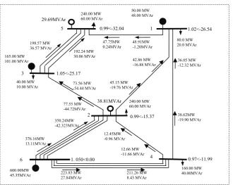
. Also, a total of 68.5 MVAr reactive sources should be

The line costs for the second solution are UM 250.000 with a different topology, n_{2 6−} =5; n_{3 5}− =2; n4 6− =2 and a total of 57.6 MVAr is needed for installation at buses 4 and 5. Active and reactive power losses are 55.00 MW and 210.40 MVAr, respectively. Figure 5 shows the complete results for this solution. Detailed investment for transmission lines, VAr sources and real power losses are given in Table 1.

Table 1 Results for the Garver System

Costs (US $)

Garver system (Solution 1)

Garver system (Solution 2)

Transmission lines ₍ 250.000

2 6 4; 3 5 2; 4 6 3

n− = n− = n− = )

250.000

(n_{2 6−} =5;n_{3 5−} =2;n_{4 6−} =2)

Power losses 55.000 55.000

VAr sources 20.750 17.480

Total 325.750 322.480

As indicated, with different topologies, transmission line costs are equal for both solutions, but solution 2 is preferred since it has a lower total investment cost. The results obtained through this example illustrate a significant realization of simultaneous transmission expansion and reactive power source allocation. Additionally, the final topology may have a reliable operation when tested with an AC power flow, so the solution may not require additional transmission line reinforcement. Such reinforcements, starting with the transmission line planning, are generally necessary when a DC model is used to handle the planning process. The solution for a DC model of this system is reported in [2, 9], where the investment cost is UM 200.000 with installation of the following lines: n_{2 6−} =4; n_{3 5}− =1; n4 6− =2. This solution falls short when

AC network is considered, however, the results obtained in this section provide the planner with the exact topology in the real system conditions (AC Network).

b) IEEE-24 bus system

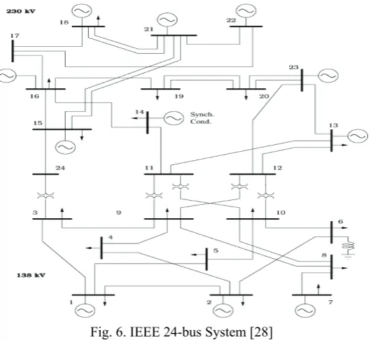
The IEEE 24-bus system data is given in [28] and depicted in Fig. 6. This system is to expand to a future condition with generation levels and the loads three times their original values (i.e, up to a total

80.0 MW 20.0 MVAr 240.00 MW 60.00 MVAr 1 5 3 2

6 4

160.00 MW 40.00MVAr 40.00 MW 10.00 MVAr 240.00 MW 60.00 MVAr 36.05 MW -12.32 MVAr 223.83 MW 27.84MVAr 211.26 MW 8.43 MVAr 12.45MW -0.96 MVAr 38.62MW -19.90 MVAr 165.00 MW 101.00 MVAr 73.56 MW -54.44 MVAr 77.55 MW -44.72MVAr 42.86 MW -16.88 MVAr 47.75MW 0.24MVAr 48.91MW -1.20MVAr 198.57 MW 36.57 MVAr 350.24MW -42.323MVAr 376.16MW 13.11MVAr 50.00 MW 48.00 MVAr 600.00MW 45.35MVAr 45.15 MW -19.76 MVAr 192.24 MW 30.06 MVAr 1.02<-26.54 0.97<-11.99 1.05<-25.17 1. 050<0.00 0.99<-15.37 0.99<-32.04 12.66 MW -11.66 MVAr 38.81MVAr 29.69MVAr

10215 Mw maximum generation capacity and 8550 Mw peak demand). Therefore there appears to be enough generation capacity, but according to [28], it is shown that new lines are required to be installed to avoid load curtailment. The IEEE 24-bus system has 24 buses and 41 transmission lines. In this case the VAr fixed cost of installation is considered to be c₀=10000 US$ and the VAr variable cost is

1 3 US$ / r

c = kVA . The cost of energy (

k

_e) is considered to be 0.06 $/KW hour and system duration time is

1*365* 24( )

D= hour for a one-year planning horizon.

Fig. 6. IEEE 24-bus System [28]

RGA is used to find the optimal solution for the TNEP-RPP in a unique stage, while twenty independent runs of RGA are implemented to find a solution. Each run of RGA converges after an average of 15 generations, solving about 210 OPF. About 40% of the runs have optimal solutions. Results are obtained

80.0 MW 20.0 MVAr

240.00 MW 60.00 MVAr

1 5

3

2

6 4

160.00 MW 40.00MVAr 40.00 MW

10.00 MVAr

240.00 MW 60.00 MVAr

25.75 MW -6.50 MVAr

190.98 MW 20.16 MVAr

177.42 MW -12.3 MVAr 9.76MW

-6.05 MVAr

27.09MW -18.77 MVAr 165.00 MW

101.00 MVAr

78.60 MW -54.98 MVAr

83.06 MW -43.23MVAr

48.38 MW -19.93 MVAr 43.16MW

3.65MVAr

44.13MW 1.57MVAr 203.61 MW

36.03 MVAr

384.15MW -9.2 MVAr

409.00MW 37.65MVAr

50.00 MW 48.00 MVAr

600.00MW 57.81MVAr

51.34 MW -19.91 MVAr 196.83 MW

27.30 MVAr

1.01<-26.11

0.97<-15.63 1.04<-23.85

1. 050<0.00

0.98<-13.25 0.98<-31.09

9.66 MW 4.94 MVAr

28.6MVAr 29.06MVAr

by the following new lines: n_{7 8}− =2; 2; 1; 1n_{6 10}− = n_{14 16}− = n_{10 12}− = . A total of 901.48 MVAr reactive sources are installed at buses 3, 8, 9, 11 and 12, with the size of 170.34, 109.14, 210.15, 172.61 and 239.23 MVAr, respectively. Active and reactive power losses are 209.15 MW and 780 MVAr, respectively. The total investment is US$ 280,684,410, which is shown in Table 2.

Table 2. Overall results for the IEEE 24-bus system

The optimum solution for DC model is reported in [9], with 152,000,000 investment on the following transmission lines:n_{7 8−} =2; 1; 1; 1n_{6 10−} = n_{14 16−} = n_{10 12−} = . However, this topology is not able to provide a viable operation when considering the complete AC network where power losses and reactive demands play an important role in the network. The solution provided for the AC model of the IEEE-24 bus system in this paper shows the importance of integrated transmission and reactive power planning. The result of the AC OPF with the proposed transmission lines and reactive sources is given in Tables 3 and 4. Table 3 shows the results related to the system buses, while Table 4 shows branch results. The voltage magnitude and angle, the real and reactive power demand, the real and reactive power generation and the allocated reactive power sources at system buses are shown in Table 3. The results related to the system branches in Table 4 contain: the existing and new transmission lines, the active, reactive and apparent power flow at each end of the transmission lines and the active and reactive power losses.

Table 3. Detailed results of the IEEE 24-buses system ( Bus View) [28]

Costs (US $) IEEE 24 Bus System

Transmission Lines ₍ 168,000,000

7 8 2; 6 10 2; 14 16 1; 10 12 1

n₋ = n₋ = n ₋ = n ₋ = )

Power Losses 109,930,000

VAr sources 2,754,410

Total 280,684,410

Bus Type _(Volt) Vm _(Rad) Teta PD

[MW] QD

[MVAr] PG

[MW] QG

[MW]

VAR [MVAr]

1 Vθ 1.03 0 324 66 569.33 -79.46 0

2 PV 1.05 -0.03 291 60 576 219.57 0

3 PQ 0.96 -11.12 540 111 0 0 170.34

4 PQ 0.96 -11 222 45 0 0 0

5 PQ 0.99 -8.16 213 42 0 0 0

6 PV 1.04 -10.07 408 84 0 -262.11 0

7 PV 1.05 -1.33 375 75 899.19 104.11 0

8 PQ 1.02 -6.98 513 105 0 0 109.14

9 PQ 1.01 -7.32 525 108 0 0 210.15

10 PQ 1.05 -6.65 585 120 0 0 0

11 PQ 1.04 8.17 0 0 0 0 172.61

12 PQ 1.02 7.64 0 0 0 0 239.23

13 PV 1.05 20.23 795 162 1489.42 274.21 0

14 PV 1.05 12.58 582 117 0 331.91 0

15 PV 1.03 22.01 951 192 645 330 0

16 PV 1.04 20.91 300 60 465 240 0

17 PQ 1.04 27.78 0 0 0 0 0

18 PV 1.05 31.11 999 204 1180.91 232.95 0

19 PQ 1.01 21.57 543 111 0 0 0

20 PQ 1.02 28 384 78 0 0 0

21 PV 1.05 32.89 0 0 1149.40 5.19 0

22 PV 1.05 31.17 0 0 13.53 -13.50 0

23 PV 1.05 33.53 0 0 1771.38 236.59 0

24 PQ 0.95 10.14 0 0 0 0 0

Table 4. Detailed result of the IEEE 24-buses system ( Branch View) [28]

from to Nij Nij0 _[MW] Pij _[MW] Qij _[MW] Sij _[MW] Pjj _[MW] Qji _[MW] Sji Loss P _[MW] Loss Q _[MW] Sij max

[MW]

1 2 0 1 -24.34 -173.30 175 24.90 126.44 128.87 0.56 -46.86 175 1 3 0 1 94.99 17.23 96.54 -90.13 -4.06 90.22 4.86 13.17 175 1 5 0 1 174.68 10.61 175 -168.37 11.50 168.76 6.31 22.11 175 2 4 0 1 163.71 46.42 170.16 -155.04 -16.40 155.91 8.67 30.02 175 2 6 0 1 96.39 -13.29 97.30 -92.15 23.98 95.22 4.24 10.69 175 3 9 0 1 -60.19 -26.85 65.90 61.63 29.30 68.24 1.44 2.46 175 3 24 0 1 -389.69 90.25 400 393.72 56.87 397.80 4.03 147.11 400 4 9 0 1 -66.96 -28.60 72.81 68.48 31.79 75.50 1.53 3.19 175 5 10 0 1 -44.63 -53.50 69.67 45.72 55.25 71.71 1.09 1.74 175 6 10 2 1 -315.85 -370.09 486.55 320.16 -416.08 525 4.31 -786.17 525 7 8 2 1 524.19 29.11 525 -510.93 16.74 511.21 13.26 45.85 525

8 9 0 1 5.55 4.79 7.33 -5.52 -9.27 10.79 0.03 -4.48 175

8 10 0 1 -7.62 -17.39 18.98 7.73 13.04 15.16 0.12 -4.35 175 9 11 0 1 -332.71 18.52 333.22 335.22 73.08 343.09 2.51 91.60 400 9 12 0 1 -316.89 31.82 318.48 319.18 51.86 323.37 2.29 83.68 400 10 11 0 1 -330.41 66.58 337.05 332.78 19.91 333.37 2.37 86.49 400 10 12 1 1 -628.21 161.22 648.57 632.60 -1.10 632.60 4.39 160.12 800 11 13 0 1 -467.67 79.68 474.41 480.46 9.18 480.54 12.78 88.86 500 11 14 0 1 -200.32 -0.06 200.32 202.33 6.04 202.42 2.01 5.98 500 12 13 0 1 -484.34 55.04 487.46 498.20 42.36 500 13.86 97.41 500 12 23 0 1 -467.44 133.43 486.11 495.73 65.17 500 28.30 198.60 500 13 23 0 1 -284.24 60.66 290.64 292.87 -13.40 293.18 8.64 47.26 500 14 16 1 1 -784.33 208.87 811.67 799.36 -109.82 806.87 15.03 99.05 1000 15 16 0 1 108.51 -80.83 135.31 -108.14 79.88 134.44 0.37 -0.94 500 15 21 0 2 -819.94 81.95 824.03 840.23 53.63 841.94 20.29 135.58 1000 15 24 0 1 405.43 136.87 427.91 -393.72 -56.87 397.80 11.71 80.01 500 16 17 0 1 -492.17 69.80 497.09 499.73 -16.36 500 7.56 53.44 500 16 19 0 1 -34.05 140.13 144.21 34.65 -140.61 144.82 0.60 -0.48 500 17 18 0 1 -438.70 24.46 439.38 441.89 -2.28 441.90 3.19 22.18 500 17 22 0 1 -61.03 -8.10 61.57 61.49 -12.54 62.76 0.46 -20.64 500 18 21 0 2 -259.98 31.23 261.85 261.01 -35.15 263.37 1.03 -3.92 1000 19 20 0 2 -577.65 29.61 578.41 586.05 18.44 586.34 8.40 48.05 1000 20 23 0 2 -970.05 -96.44 974.83 982.77 184.82 1000 12.72 88.37 1000 21 22 0 1 48.15 -13.29 49.95 -47.96 -0.96 47.97 0.19 -14.26 500

Total 6 209.15 780.92

6. CONCLUSION

REFERENCES

1. Gajbhiye, R. K., Naik, D., Dambhare, S. & Soman, S. A. (2008). An expert system approach for multi-year short-term transmission system expansion planning: An Indian experience. Power Systems, IEEE Transactions on, Vol. 23, No. 1, pp. 226-237.

2. Romero, R., Monticelli, A., Garcia, A. & Haffner, S. (2002). Test systems and mathematical models for transmission network expansion planning. IEE Proc. Gen. Trans. Distrib., Vol. 149, No. 1, pp. 27–36.

3. Romero, R. & Monticelli, A. (1994). A hierarchical decomposition approach for transmission network expansion planning. IEEE Trans. Power Syst., Vol. 9, No. 1, pp. 373–380.

4. Rider, M. J., Garcia, A. V. & Romero, R. (2008). Transmission system expansion planning by a branch-and-bound algorithm. IET Gener. Trans. Distrib., Vol. 2, No. 1, pp. 90–99.

5. Binato, S, Pereira, M. V. F. & Granville, S. (2001). A new Benders decomposition approach to solve power transmission network design problems. IEEE Trans. Power Syst., Vol. 16, No. 2, pp. 235–240.

6. Alguacil, N., Motto, A. L. & Conejo, A. J. (2003). Transmission expansion planning: a mixed-integer LP approach. IEEE Trans. Power Syst., Vol. 18, No. 3, pp. 1070–1077.

7. Gallego, R. A., Alves, A. B., Monticelli, A. & Romero, R. (1997). Parallel simulated annealing applied to long term transmission network expansion planning, IEEE Trans. Power Syst., Vol. 12, No. 1, pp. 181–188.

8. Gallego, R. A, Monticelli, A. & Romero, R. (1998). Transmission systems expansion planning by an extended genetic algorithms. IEE Proc. Gen. Trans. Distrib., Vol. 145, No. 3, pp. 329–335

9. Romero, R., Rider, M. J. & Silva, I. D. J. (2007). A metaheuristic to solve the transmission expansion planning. IEEE Trans. Power Syst., Vol. 22, No. 4, pp. 2289-2291.

10. Pavluchenko, D. A. & Manusov, V. Z. (2006). Electrical network optimization by genetic algorithm. Euro. Trans. Electr. Power; Vol. 16, pp. 569–576.DOI: 10.1002/etep.104

11. Da Silva, E. L., Ortiz, J. M. A., De Oliveira, G. C. & Binato, S. (2001). Transmission network expansion planning under a Tabu search approach. IEEE Trans. Power Syst., Vol. 16, No. 1, pp. 62–68.

12. Binato, S., De Oliveira, G. C. & De Araujo, J. L. (2001). A greedy randomized adaptive search procedure for transmission expansion planning. IEEE Trans. Power Syst., Vol. 16, No. 2, pp. 247–253.

13. Paulun, T. (2006).Strategic expansion planning for electrical networks considering uncertainties. Euro. Trans. Electr. Power, Vol. 16,pp. 661–671.

14. Forghani, M. A., Seyed-Esfahani, M., Rashidinejad, M. & Farahmand, H. (2008). A goal attainment model for transmission expansion planning using a meta heuristic technique. Iranian Journal of Science & Technology, Transaction B, Engineering, Vol. 32, No. B3, pp. 235-247.

15. Wenjuan, Z., Fangxing, L. I. & Tolbert, L. M. (2007). Review of reactive power planning: objectives, constraints, and algorithms. Power Systems, IEEE Transactions, Vol. 22, No. 4, pp. 2177-2186.

16. Delfanti, M., Granelli, G., Marannino, P. & Montagna, M. (2000). Optimal capacitor placement using deterministic and genetic algorithms. IEEE Trans. Power Syst., Vol. 15, No. 3, pp. 1041–1046.

17. Eghbal, M., Yorino, N., El-Araby, E. E. & Zoka, Y. (2008). Multi-load level reactive power planning considering slow and fast VAR devices by means of particle swarm optimisation. Generation, Transmission & Distribution, IET, Vol. 2, No. 5, pp.743-751.

18. Zhang, W. & Liu, Y. (2002). Optimal VAr planning in area power system. Proc. Int. Conf. Power System Technology, pp. 2072–2075.

19. Estevam, C. R. N., Rider, M. J, Amorim, E. & Mantovani, J. R. S. (2010). Reactive power dispatch and planning using a non-linear branch-and-bound algorithm. Generation, Transmission & Distribution, IET, Vol. 4, No. 8, pp.963-973.

21. Rahmani, M., Rshidienjad, M. & Romero, R. (2010). Efficient method for AC transmission network expansion planning. Electric Power Systems Research, Vol. 80, No. 9, pp. 1056-1064.

22. Rider, M. J., Garcia, A. V. & Romero, R. (2007). Power system transmission network expansion planning using AC model. IET Gener. Transm. Distrib., 2007, 1 (5), pp. 731–742.

23. Rahmani, M., Rashidinejad, M., Carreno, E. M. & Romero, R. A. (2010). A combinatorial approach for transmission expansion & reactive power planning. Transmission and Distribution Conference and Exposition: Latin America (T&D-LA), 2010 IEEE/PES, pp.529-536.

24. Goldberg, D. E. (1989). Genetics algorithms in search, optimization and machine learning. Addison–Wesley. 25. Niknam, T., Ranjbar, A. M., Shirani, A. R. & Ostadi, A. (2005). A new approach based on ANT algorithm for

volt/var control in distribution network considering distribution generation. Iranian Journal of Science & Technology, Transaction B, Engineering, Vol. 29, No. B4.

26. Li-Xin, W. (1997). A course in fuzzy systems and control. Prentice Hall.

27. Choi, J, El-Keib. A. A. & Tran, T. (2005). A fuzzy branch and bound-based transmission system expansion planning for the highest satisfaction level of the decision maker. IEEE Trans. Power Syst., Vol. 20, No. 1, pp. 475-484.

28. Fang, R. & Hill, D. J. (2003). A new strategy for transmission expansion in competitive electricity markets.

IEEE Trans. on Power Systems, Vol. 18, No. 1, pp. 374–380.

29. Poonpun, P. & Jewell, W. T. (2008). Analysis of the cost per kilowatt hour to store electricity. Energy Conversion, IEEE Transactions on, Vol. 23, No. 2, pp.529-534.

30. http://www.eia.gov/electricity/wholesale/index.cfm

31. De la Torre, S., Conejo, A. J. & Contreras, J. (2008). Transmission expansion planning in electricity markets.