A Stochastic Operational Planning Model for Smart Power
Systems
S. Jadid*(C.A.) and S. A. Bahreyni*
Abstract: Smart Grids are result of utilizing novel technologies such as distributed energy resources, and communication technologies in power system to compensate some of its defects. Various power resources provide some benefits for operation domain; however, power system operator should use a powerful methodology to manage them. Renewable resources and load add uncertainty to the problem. So, independent system operator should use a stochastic method to manage them. A Stochastic unit commitment is presented in this paper to schedule various power resources such as distributed generation units, conventional thermal generation units, wind and PV farms, and demand response resources. Demand response resources, interruptible loads, distributed generation units, and conventional thermal generation units are used to provide required reserve for compensating stochastic nature of various resources and loads. In the presented model, resources connected to distribution network can participate in wholesale market through aggregators. Moreover, a novel three-program model which can be used by aggregators is presented in this article. Loads and distributed generation can contract with aggregators by these programs. A three-bus test system and the IEEE RTS are used to illustrate usefulness of the presented model. The results show that ISO can manage the system effectively by using this model.
Keywords: Aggregator, Demand Response, Distributed Energy Resource, PV Farm, Stochastic Unit Commitment, Wind Farm.
1 Introduction 1
Smart Grids are result of using novel technologies in power system. This integration enhances some features of power systems; it provides essential infrastructure for performing demand response program, and it improves the condition for utilizing high penetration of distributed generation. Also, nowadays, renewable resources are considered as significant resources for electric power generation in smart grids. These new elements provide more options for power system operator in order to supply demand.
The new power resources help power system operator to provide power demand more environmental and economical, and with higher power quality. In order to achieve these goals, Independent System Operator (ISO) should manage these resources effectively. ISO can choose between various options for providing demand. Most of these resources are uncertain; for
Iranian Journal of Electrical & Electronic Engineering, 2014. Paper first received 6 Nov. 2014 and in revised form 2 July 2014. * The Authors are with the Center of Excellence for Power System Automation and Operation, Department of Electrical Engineering, Iran University of Science and Technology, Tehran, Iran.
E-mails: [email protected] and [email protected].
instance, renewable resources and demand response resources are not completely predictable. Renewable generations are thoroughly dependent to the weather condition. Interruptible load may deny reducing their consumption when it is essential. In order to accommodate the uncertain nature of these resources, scheduling in an electricity market [1, 2] need to be modified during the actual operation of the power system. The reserves are the ancillary services traded in the market to overcome these uncertainties.
As the amount of uncertainties increase, the requirement for spinning and non-spinning reserves increases [3], and this increase causes higher operation cost. So, operator and planner must tradeoff between the advantages of using these resources and their disadvantage (increasing cost by raise in essential reserves level).
To this end, an appropriate optimization model is essential to determine the amount of power which should be produced by each of generation resources and the amount of required reserve. Many valuable works has been done to determine optimal amount of power generation and reserves by each generation unit. The traditional criterion for adjusting the minimum amount
of the spinning reserve requirement is that it should be greater than or equal to the capacity of the largest online generating unit [4]. This criterion guarantees that no load has to be curtailed if any single generating unit is unexpectedly disconnected. However, this deterministic method opposes the economic principles. The intermittency and unpredictability of renewable power generation and other power resources make some difficulties in control of frequency. So, using an effective method for power system operational scheduling seems essential.
A considerable number of unit commitment approaches has been submitted, especially in recent years. Some of them [5-11], model a security-constrained UC. Paper [5, 6] offers a stochastic security market-clearing problem which defines the involuntary load shedding and reserve services in a way that pre-contingency social welfare and expected operating costs would be optimized. In this method, expected cost is reduced but instead, an amount of energy not supplied is resulted because scheduling for more reserves would not be economical. Paper [7] proposes an approach for generation scheduling using sensitivity characteristic of a Security Analyzer Neural Network (SANN) for improving static security of power system. Furthering the previous model, [8] and [9] has considered variable wind power sources in a stochastic SCUC model, but yet other distributed resources like solar resources was not considered. In [8], a market clearing mechanism is formulated as a stochastic optimization problem where the net demand forecast error is modeled as a normally distributed random variable. A relevant paper on wind-thermal scheduling problem is [12]; air pollutants emission level and operating costs are considered as two objective functions of a multi-objective mathematical programming model. Paper [13], proposes a benders decomposition approach to solve thermal unit commitment problem. The model is divided to master mixed integer problem and a nonlinear sub-problem and a comparison for different methods is also proposed.
Moving toward smart grids, [10, 11] have considered the impact of demand response on the hourly operation and control of constrained power systems; papers [11, 14], have used demand response providers to aggregate the costumer responses. Reserve provided by demand response and spinning reserve is scheduled in this stochastic model. [15, 16] aimed to minimize the expected cost and air pollutant emission during UC scheduling for a set of scenarios; some renewable energy sources and plug-in hybrid electric vehicles are considered during this scheduling. Although these papers consider UC with gridable vehicles and emission reduction objective, they use a deterministic approach resulting in non-optimal reserve level and extra operation cost.
Assorted elements of smart grids will be utilized in diverse levels. Many of them will be used by domestic customers. Renewable generation resources such as
wind micro turbine, PV panels, batteries, and electric vehicles are some of these resources. In addition, customers who will use AMI can participate in demand response programs; they will be able to manage their energy usage. Domestic customers will be able to provide their own energy; also, they will be able sell their extra energy to other consumers. Moreover, one of the main goals of smart grids is to use distributed generation instead of bulk power generation units. So, many policies are written with the aim of encouraging investor to invest in distributed generation units. These units are desirable for providing local loads; however, they can sell their extra electric power to upper-hand grid.
The amount of electric energy produced by domestic customers and distributed generations are not substantial to participate in wholesale market directly. Aggregators are service providers who can work with low power generators and customers connected to distribution network and bid their aggregated power to wholesale market [17]. In addition, customers who are connected to distribution network can sell their energy consumption reduction through aggregators. Large factories which are connected to transmission network directly can participate in wholesale market as interruptible loads. Interruptible loads can bid for reducing their power consumption which works the same as power generation. They can bid their demand reduction as electric power production or as reserve. Interruptible loads can only reduce their power consumption in discrete steps because they have to turn off a part of production process for reducing their power consumption.
Using renewable energies for producing power is requisite in smart grids. These resources will be used in both distributed generation form and in the form of massive plant. So, other resources which should be considered by ISO for producing power are vast renewable plants. Wind and PV farms are two common power generation plants in smart grid paradigm.
The innovations of this paper are highlighted as follows:
• Setting presents a pragmatic model for interruptible loads which represents actual behavior of large scale costumers.
• Introducing a novel model for aggregators’ contracts with domestic loads and distributed generation.
• Considering a scenario-based uncertainty model for wind and solar power generation, load prediction and the interruptible loads.
In this paper, a stochastic UC model considering aggregator bids, bids from thermal units, and wind and PV generations is presented. Renewable generation outputs, interruptible loads, and load predictions are considered as elements which contain uncertainty. This
stochastic model calculates sufficient amount of reserve from appropriate resources for covering uncertainties. In addition, a novel model for aggregators’ contracts is presented. In the next sections, the model is presented; then, the presented model is tested in a three-bus case study and IEEE RTS system. Also, the results are discussed. Finally, a conclusion is presented.
2 Model
As explained in the introduction, ISO can use various resources to provide power demand. Conventional units, renewable farms, interruptible loads, and aggregators are some of these resources. In addition, ISO can provide required amount of reserve through various resources. Conventional units, interruptible loads, and aggregators are appropriate resources for providing required amount of reserve. In order to avoid probable misleading solutions resulted from deterministic programming, we modeled stochastic nature of Wind, PV, load, and interruptible load through scenario based uncertainty modeling. A common way of solving problems of stochastic programming type is to perform scenario analysis, which is counted as one of the methods for solving stochastic problems [18]. In this part, a stochastic optimization model is used to calculate appropriate amount of reserve from each resource.
2.1 Objective Function
The objective function in the presented model is minimization of expected cost for providing the required power and reserve from diverse resources. It is given below in Eq. (1). The notation is observable in the appendix.
Each line of objective function is explained below: 1. Start-up cost of the conventional generating units; 2. The energy offer cost of the generating units minus
the demand utility;
3. The offer cost of contracting up/down spinning and non-spinning reserves from conventional generating units;
4. The offer cost of wind and PV farms;
5. The energy and reserve offer cost of interruptible loads; It is considered that these customers are large industrial loads that have bought their required demand through long-term contracts.
6. The energy and reserve offer cost of aggregators; 7. The cost resulting from the changes of the start-up
and shut-down plan of generating units in each scenario;
8. The cost associated to the actual use of reserve from generating units;
9. The cost associated to the actual use of reserve from interruptible loads and aggregators;
10. The cost of the load shedding;
(
)
(
,)
1 1
,
1 1 1
, , , 1 , , 1 1 , 1 t C
t C L
jt
C
U D NS
WP PV
DR DR DR S dt dt N N
it t i
N N N
C C S L S
t it it jt
t i j
N
C R U C R D C R NS it it it it it it i
N N
WP WP S PV PV S vt vt pt pt
v p
N
DR R DR dt dt d
p R
Cost
SUC
d p L
R R R
p p
λ λ
λ λ
λ λ λ
λ λ = = = = = = = = = + + + = ⎡ − ⎢ ⎢⎣ + + + + +
∑∑
∑ ∑
∑
∑
∑
∑
(
, ,)
1 ,1 1 1
, 1 1 , , 1 1 , 1 Ag
w t C
t C
Ag DR
L N
Ag Ag S Ag R Ag at at at at a
N N N
A
w it w
w t i
N N
C C t it it w
t i
N N
DR DR Ag Ag dt dt w at at w
d a
N
jt jt w j p R SUC d r r r VOLL LC λ λ ρ λ λ λ = = = = = = = = = + + ⎤⎥ ⎥⎦ ⎧⎪ + ⎨ ⎪⎩ ⎡ + ⎢ ⎢⎣ + + ⎫ ⎤⎪ + ⎥⎬ ⎥⎪ ⎦⎭
∑
∑
∑ ∑∑
∑ ∑
∑
∑
∑
(1)2.2 Electricity Market Constraints
1- Market Balance:
, , ,
1 1 1
, ,
1 1 1
.
C WP PV
Ag
DR L
N N N
C S WP S PV S
it wt pt
i w p
N
N N
DR S Ag S S
dt at jt
d a j
p p p
p p L t
= = = = = = + + + + = , ∀
∑
∑
∑
∑
∑
∑
(2)As it is mentioned before, conventional units, wind and PV farms, interruptible loads, and aggregators can provide required power. Network constraints are not considered in the representation of the market. So, network constraints are only enforced in the actual operation of the power system.
2- Production Limits:
,min , ,max
,
C C C S C C
i it it i it
p Ι ≤p ≤p Ι , ∀ ∀i t (3)
3- Wind and PV Generation Limits:
,min , ,max
,
W P W P W P S W P W P
vt vt vt vt vt
p Ι ≤ p ≤p Ι , ∀ ∀v t
(4)
,min , ,max
,
PV PV PV S PV PV
pt pt pt pt pt
p Ι ≤p ≤p Ι , ∀ ∀p t (5)
where W P,max
vt
p and W P,min
vt
p are parameters submitted as part of the wind plant energy offer.
4- Interruptible loads:
The proposed model for interruptible loads is one of the innovations of this paper. Interruptible loads should curtail some parts of their electricity usage if they are committed in power and reserve provision. For instance, a factory, when needed, should turn off a production line for being considered as power producer in power balance equation. So, interruptible loads can reduce their electricity usage in discrete manner. In other words, ISO should consider this limit in power system operational planning; ISO should allocate logical energy production amount to interruptible loads. This limit would be announced by interruptible loads as a part of their bid to energy market while the minimum limit should be confirmed by ISO. This limit is illustrated in Eqs. (6) and (7).
,
DR S DR
dt dt d
p =
α
p , ∀ ∀d t (6)min max
,
DR S DR
d dt dt d dt d t
α Ι ≤α ≤α Ι , ∀ ∀ (7)
where αdtis an integer
5- Demand Bounds:
,min ,max
,
S S S
jt jt jt
L ≤L ≤L , ∀ ∀ j t (8)
In the case of inelastic demand, the two limits are equal, that is, LSjt,min =LSjt =LSjt,max.
6- Scheduled Reserve Determination Constraints: a) Generation-side:
Spinning reserve:
,max
0≤RUit ≤RitU Ι , ∀ ∀Cit i, t (9)
,max
0≤RitD ≤RitD Ι , ∀ ∀Cit i, t (10)
Non-spinning reserve:
(
)
,max
0≤RitNS ≤RitNS 1− Ι , ∀ ∀Cit i, t (11) b) Interruptible loads:
,max
0≤RdtDR ≤RdtDR , ∀ ∀d, t (12) 7- Aggregators’ constraint:
As it is mentioned in previous sections, DG owners and domestic customers who have AMI or/ and micro-generation units can participate in wholesale market by making contracts with aggregators. A novel model including three types of contracts is presented in this paper. Aggregators define three types of contracts; DG owners and customers can select the most desirable contract and accept all aspects of it. Customers or DG owners who choose these three contracts accept to provide only reserve, only energy and both reserve and energy, respectively in these three contracts, if aggregator is selected by ISO. Eqs. (13-19) show aggregators’ constraints which should be considered by ISO.
2,min 2, 2,max
,
Ag Ag Ag S Ag Ag
at at at at at
p Ι ≤ p ≤p Ι , ∀ ∀a t (13)
3,min 3, 3,max
,
A g A g A g S A g A g
at at at at at
p Ι ≤p ≤p Ι , ∀ ∀a t (14)
, 2, 3,
,
A g S A g S A g S
at at at
p = p +p , ∀ ∀a t (15)
1,min 1 1,max
,
R R
Ag A g A g A g Ag
at at at at at
R Ι ≤R ≤R Ι , ∀ ∀a t (16)
3,min 3 3,max
,
R
A g A g A g A g
at at at at
R Ι ≤R ≤R , ∀ ∀a t (17)
1 3
,
A g A g A g
at at at
R =R +R , ∀ ∀a t (18)
3,max 3,max 3,
,
R
A g A g Ag A g S
at at at at
R =p I −p , ∀ ∀a t (19)
8- Start-Up Cost:
(
, 1)
,SU C C
it i it i t
SUC ≥λ Ι − Ι − , ∀ ∀i t (20)
0 ,
it
SUC ≥ , ∀ ∀i t (21)
2.3 Actual System Operation Constraints
1- Power Balance Constraints: a) Power Balance at Every Node n:
, ,
:( , ) :( , )
, ,
:( , ) :( , )
, ,
:( , ) :( , )
, ,
:( , )
( , )
( ) 0,
, ,
G w
p d
a L
C WP
it w wt w
i i n M w w n M
PV DR
pt w dt w
p p n M d d n M
Ag
at w t w
a a n M r n r
jt w jt w
j j n M
p p
p p
p f n r
L LC
n t w
∈ ∈
∈ ∈
∈ ∈Λ
∈
+ +
+ +
−
− − =
∀ ∀ ∀
∑
∑
∑
∑
∑
∑
∑
(22)
where pW Pwt w, , PV, pt w p , DR,
dt w
p and A g, at w
p are considered to be zero at this equation except at nodes in which their power generation is injected.
b) Power flow through line (n, r) from n to r:
, ,
, ,
( , ) ( , )
2
( , )( ), ( , ) , ,
loss t w t w
nt w rt w
P n r f n r
B n r δ δ n r t w
= +
− ∀ ∈ Λ ∀ ∀
(23)
2- Generation Limits:
,min ,max
, , , , ,
C CW C C CW
i it w it w i it w i t w
p Ι ≤ p ≤ p Ι , ∀ ∀ ∀ (24) 3- Aggregators limit:
The only aggregators’ contract including both energy and reserve contract is the third one.
3,min 3 3,max
, , , , ,
Ag A gW Ag Ag AgW
at at w at w at at w
p Ι ≤p ≤p Ι , ∀ ∀ ∀a t w (25)
4- Transmission Capacity Constraints:
max max
,
( , ) ( , ) ( , ),
( , ) , ,
t w
f n r f n r f n r
n r t w
− ≤ ≤
∀ ∈ Λ ∀ ∀ (26)
5- Uncontrolled Load Shedding Constraints:
,
0≤LCjt w ≤LSjt, ∀ ∀ ∀j, t, w (27) Amount of load shedding is determined based on value of loss load (VOLL) and the operation cost in each scenario with taking into consideration their probabilities.
2.4 Constraints Linking the Market and the Actual System Operation
1- Determining optimal amount of up, down, and non-spinning reserves from conventional units:
,
0≤rit wU ≤RUit , ∀ ∀ ∀i, t, w (28)
,
0≤rit wD ≤RitD, ∀ ∀ ∀i, t, w (29)
,
0≤rit wNS ≤RitNS, ∀ ∀ ∀i, t, w (30)
, , , , , ,
U NS D C
it w it w it w it w
r +r −r =r , ∀ ∀ ∀i t w (31)
, ,max ,
, , ,
C S C C C S
it it w i it
p r p p i t w
− ≤ ≤ − , ∀ ∀ ∀ (32)
2- Determining optimal amount reserves from aggregators:
1 1
,
0≤rat wA g ≤RatA g , ∀ ∀ ∀a, t, w (33)
3 3
,
0≤rat wAg ≤RatAg , ∀ ∀ ∀a, t, w (34)
1 3
, , , , ,
A g A g A g
at w at w at w
r +r =r , ∀ ∀ ∀a t w (35)
3- Determining optimal amount reserves from interruptible loads:
,
0≤rdt wDR ≤RdtDR, ∀ ∀ ∀d, t, w (36) 4- Second-Stage Start-Up Cost Adjustments:
, , , , ,
A
it w it w it
SUC =SUC −SUC ∀ ∀ ∀i t w (37)
(
)
, , , 1, , ,
SU S S
it w i it w i t w
SUC ≥λ Ι − Ι − , ∀ ∀ ∀i t w (38)
, 0 , ,
it w
SUC ≥ , ∀ ∀ ∀i t w (39)
5- Decomposition of the Power Consumed by each Load:
, , , , , ,
C S U D
jt w jt jt w jt w
L =L −r +r ∀ ∀ ∀j t w (40)
6- Deployed Reserve Determination Constraints:
,
0≤rjt wU ≤RUjt, ∀ ∀ ∀j, t, w (41)
,
0≤rjt wD ≤RDjt, ∀ ∀ ∀j, t, w (42)
3 Numerical Results
The proposed model is examined through two test system. A modified three-bus test system and IEEE RTS test system [19] have been used in this paper in order to show usefulness of the model. The optimization was solved by using the mixed-integer linear programming solver CPLEX 9.0 under GAMS [20] and had been implemented on a Pentium IV, 2.00 GHz processor with 2 GB of RAM.
The data of modified three-bus test system is taken from [21]. The hourly demand, which is considered to be in bus 3, is 30, 80, 110, and 40 MW, respectively. The value of lost load is considered to be 1000 $/MWh. Data of conventional generation units is given in Table 1; these data is taken from [21].
Table 1Generator data three-bus system.
Generator No. i
1 2 3
,min
C i p
(MW) 10 10 10
,max
C i p
(MW) 100 100 50
it
S UC ($) 100 100 100 C
it
λ
($/MWh) 30 40 20
, U
C R it λ
($/MWh) 5 7 8
, D
C R it λ
($/MWh) 5 7 8
, NS
C R it
λ ($/MWh) 4.5 5.5 7
A wind farm is considered in bus 2 in this test system. A wind farm is considered in bus 2 in this test system. The wind power generation is predicted to be 6, 20, 35, and 8 MW, respectively. These predictions are equal to wind power prediction in [21].
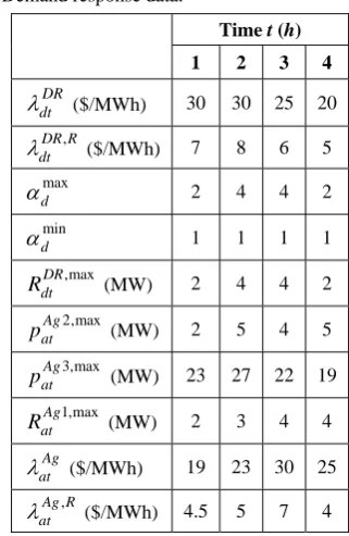
A solar generation units is considered to be in bus 1. The generation prediction of this unit is considered to be 4, 10, 5, and 0 MW, respectively. A large consumer such as a factory which is connected to transmission system can participate in wholesale market and offer its electricity usage as a power or/and reserve provider. These types of consumers can provide their power and energy through their local power generation units (such as diesel generators) or their electricity usage reduction. Most of large consumers provide important part of their electricity usage through long-term contracts. Later, they can reduce and sell a part of their electricity usage as power or reserve. Some of these large consumers offer power and reserve to wholesale market. ISO decide whether they should reduce their electricity usage base on its main goal (lower cost in presented model). Interruptible loads can reduce their electricity usage as pre-specified intervals. For instance, in this case study, the interruptible loads can reduce 1 MW or 2 MW of their electricity usage in hour 1; however, it is impossible for it to reduce 1.5 MW. As it is explained in previous section, the reason of this interval is that load should turn off or curtail one part of its production chain; so, it is impossible for it to reduce their electricity usage in continuous amount. Data of this interruptible load is given in Table 2. In other words, DR
d
p is
considered to be 1 MW, and αdtS is assumed as a
discrete variable which varies between a minimum and maximum in each hour. As it is explained in previous section, DG owner and consumers which are connected to distribution network can participate in wholesale markets through aggregators. Data of such aggregators are illustrated in Table 2.
Table 2 Demand response data.
Time t (h)
1 2 3 4
DR dt
λ ($/MWh) 30 30 25 20 ,
DR R dt
λ ($/MWh) 7 8 6 5 max
d
α 2 4 4 2
min
d
α 1 1 1 1
,max
DR dt
R (MW) 2 4 4 2
2,max
Ag at
p (MW) 2 5 4 5
3,max
Ag at
p (MW) 23 27 22 19 1,max
Ag at
R (MW) 2 3 4 4
Ag at
λ ($/MWh) 19 23 30 25 ,
Ag R at
λ ($/MWh) 4.5 5 7 4
Minimum power generation limit for second and third program is considered to be zero. Also, minimum reserve of first and third program is considered to be zero. In this model, wind generation, solar generation, load, and interruptible load power are considered as uncertain variables. Each of these variables may have three discrete amounts in each hour. For instance, wind generation can be 4 MW (low), 6 MW (as predicted), and 9 MW (high) in first hour. The uncertainty of wind
generation unit, solar generation unit, and load is considered as follows: Wind power expected values are 100, 150 and 70 percent of the predicted value with probability of 0.6, 0.2 and 0.2 respectively. The predicted solar power value is multiplied by 100, 120 and 80 percent whiles 0.7, 0.15 and 0.15 are probability of each amount, respectively, and load uncertain sates is considered to be 100, 105, 95 percent of the predicted value with probability of 0.6, 0.2 and 0.2, respectively. Although interruptible loads may accept to reduce their electricity usage, their main goal is to produce their own production and increase their benefit. So, they may refuse to reduce their electricity usage in real time because of various reasons. As a result, ISO should consider this uncertainty in order to improve security of operational scheduling. Interruptible load may reduce its electricity usage according to its contract with probability of 0.8; however, it may reduce its usage in amount of 1 MW lower than its contract with probability of 0.2. Although two scenarios are considered in this case study for electricity usage reduction of interruptible loads, any other models can be used for this purpose without any important changes. With these consumptions for uncertainties, this case study will have 54 (2×3×3×3) scenarios.
The results of operational planning are shown in Tables 3 and 4. These tables show power generation and reserve scheduling respectively. It is clear that wind and PV generation units are adjusted on as predicted value except for solar generation in period 3. Third conventional unit is a low cost unit. As it is illustrated in Table 3, this unit is assigned to produce power through the scheduling period.
Table 3 Power generation operational scheduling.
Table 4 operational scheduling for reserve.
Period t DR dt
R
(MW)
Ag at
R (MW) RitU (MW) RitD (MW) RitNS (MW)
1st prog. 2nd prog. 3rdprog. G1 G2 G3 G1 G2 G3 G1 G2 G3
1 1.000 0 0 3.300 0 0 0 0 0 0 5.300 0 0
2 1.000 0 0 11.000 0 0 0 0 0 16.000 0 0 0
3 4.000 3.000 0 10.000 0 0 0 0 0 24.000 0 0 0
4 2.000 0 0 3.400 0 0 0 0 0 6.000 0 0 0
Period t
,
WP S vt
p
(MW)
,
PV S pt
p
(MW)
,
DR S dt
p (MW)
Ag at
p (MW) pC Sit, (MW) 1st prog. 2nd prog. 3rd prog. G1 G2 G3
1 6.000 4.000 0 0 0 4.700 0 0 15.300
2 20.000 10.000 0 0 0 0 0 0 50.000
3 35.000 5.000 4.000 0 4.000 12.000 0 0 50.000
4 8.000 0 0 0 0 0 0 0 32.000
Due to the high amount of electricity demand in period two and three, third units is scheduled on its maximum value. Because of higher electricity demand in period 3, interruptible load, which has lower cost than conventional units except unit 3, is scheduled to produce power in maximum available power. Even by producing power by unit 3, interruptible load, wind, and PV generation, the electricity demand will not be met. So, the first conventional unit which has lower cost than the second is adjusted to produce power in the third period of time. In addition, aggregator is assigned to produce power in the first period of time because the offered cost of it is rather low in this period.
As it is illustrated in Table 4, aggregator and interruptible load are assigned to provide reserve in most periods of time. The amount of assigned up-spinning reserve is determined through stochastic program while various scenarios are considered; these assigned amounts cover diverse uncertainties in each period of time. In most of time intervals, the third unit is assigned to provide down-spinning reserve. In period 1, 2, and 4, conventional units are not assigned to provide up-spinning reserve. In these periods, unit 3 is the only conventional unit which is committed in providing power. Due to the high offered up-spinning reserve cost of this unit, it is not committed in providing up-spinning reserve. In the third period, the unit 1 is committed in providing power; so, it will be turned on in this period and can participate in providing spinning reserve. As this unit offered lower cost for up-spinning reserve than aggregator, this unit is assigned to provide up-spinning reserve in this time interval.
The results of operational planning are shown in Tables 3 and 4. These tables show power generation and reserve scheduling respectively. It is clear that wind and PV generation units are adjusted on as predicted value except for solar generation in period 3. Third conventional unit is a low cost unit. As it is illustrated in Table 3, this unit is assigned to produce power through the scheduling period. Due to the high amount of electricity demand in period two and three, third units is scheduled on its maximum value. Because of higher electricity demand in period 3, interruptible load, which has lower cost than conventional units except unit 3, is scheduled to produce power in maximum available power. Even by producing power by unit 3, interruptible load, wind, and PV generation, the electricity demand will not be met. So, the first conventional unit which has lower cost than the second is adjusted to produce power in the third period of time. In addition, aggregator is assigned to produce power in the first period of time because the offered cost of it is rather low in this period.
As it is illustrated in Table 4, aggregator and interruptible load are assigned to provide reserve in most periods of time. The amount of assigned up-spinning reserve is determined through stochastic program while various scenarios are considered; these assigned amounts cover diverse uncertainties in each
period of time. In most of time intervals, the third unit is assigned to provide down-spinning reserve. In period 1, 2, and 4, conventional units are not assigned to provide up-spinning reserve. In these periods, unit 3 is the only conventional unit which is committed in providing power. Due to the high offered up-spinning reserve cost of this unit, it is not committed in providing up-spinning reserve. In the third period, the unit 1 is committed in providing power; so, it will be turned on in this period and can participate in providing spinning reserve. As this unit offered lower cost for up-spinning reserve than aggregator, this unit is assigned to provide up-spinning reserve in this time interval.
The data of IEEE RTS system is taken form [19]. A wind farm and a PV farm are considered to be installed in bus 9 and 20 respectively. The 24 hour wind and PV generation forecast is considered as the following sets:
144,170,176,182,184,184,200, 200, 178,164,200,192,184,180,178,132,
104,108,110,105,106,156,182,152
W F
⎧ ⎫
⎪ ⎪
= ⎨ ⎬
⎪ ⎪
⎩ ⎭
0, 0, 0, 0, 0, 0, 0.4,122,220, 252,266,
250, 257,224,68,91,0, 0, 0, 0, 0, 0, 0, 0
SF= ⎨⎧ ⎫⎬
⎩ ⎭
(43)
where WF and SF represent wind and solar power forecast in MW respectively.
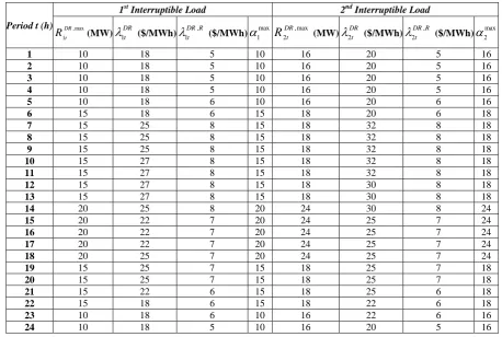
It is considered that two industrial loads have nominated for acting as interruptible loads. These interruptible loads are located in buses 3 and 18 respectively. The essential data of the interruptible loads are illustrated in Table 5. Three aggregators are considered in this test system. This assumption means that aggregators work in only three areas; consumers and distributed generations which are located in these areas can participate in wholesale market and offer their energy consumption reduction and their generation. These aggregators are located in buses number 3, 15, and 18. Essential data of these aggregators are illustrated in Table 6.
The uncertainty of wind generation, solar generation, load prediction and the interruptible loads are considered as in 3-bus test system. The proposed unit commitment model without elements of smart grid such as interruptible loads, distributed generations, demand response, and aggregators has been tested on IEEE RTS test system; the result of this test is compared with the result of proposed model while elements of the smart grid are included. The results show 3.2% decrease in total operation costs. Operation cost includes conventional and renewable generation cost and reserve cost. The total power generation cost is reduced from 678497.082$ to 656147.070$ and the total reserve cost is also reduced from 34362.435$ to 33852.015$ by using Smart Grid technologies. Fig. 1 compares the scheduled reserves for 24 hours both with and without smart grid. It is illustrated that using smart grid and the proposed method for its management, reduce operation cost while increase the amount of reserve and security.
Table 5 Hourly interruptible load data.
Period t (h)
1st Interruptible Load 2nd Interruptible Load
,max 1
DR t
R (MW)
λ
1DRt ($/MWh)λ
1DR Rt , ($/MWh)α
1max R2DRt ,max (MW)λ
2DRt ($/MWh)λ
2DR Rt , ($/MWh)α
2max1 10 18 5 10 16 20 5 16
2 10 18 5 10 16 20 5 16
3 10 18 5 10 16 20 5 16
4 10 18 5 10 16 20 5 16
5 10 18 6 10 16 20 6 16
6 15 18 6 15 18 20 6 18
7 15 25 8 15 18 32 8 18
8 15 25 8 15 18 32 8 18
9 15 25 8 15 18 32 8 18
10 15 27 8 15 18 32 8 18
11 15 27 8 15 18 32 8 18
12 15 27 8 15 18 30 8 18
13 15 27 8 15 18 30 8 18
14 20 25 8 20 24 30 8 24
15 20 22 7 20 24 25 7 24
16 20 22 7 20 24 25 7 24
17 20 22 7 20 24 25 7 24
18 20 25 7 20 24 25 7 24
19 15 25 7 15 18 25 7 18
20 15 25 7 15 18 25 7 18
21 15 22 6 15 18 25 6 18
22 15 18 6 15 18 22 6 18
23 10 18 6 10 16 22 6 16
24 10 18 5 10 16 20 5 16
Table 6 Hourly aggregators data.
t (h)
1st Aggregator 2nd Aggregator 3rd Aggregator
2,max 1
Ag t
p
(MW)
3,max 1
Ag t p
(MW)
1,max 1
Ag t
R
(MW)
1
Ag t
λ
($/MWh)
, 1
Ag R t
λ
($/MWh)
2,max 2Agt
p
(MW)
3,max 2
Ag t
p
(MW)
1,max 2
Ag t
R
(MW)
2
Ag t λ
($/MWh)
, 2
Ag R t λ
($/MWh)
2,max 3
Ag t
p
(MW)
3,max 3
Ag t
p
(MW)
1,max 3Agt
R
(MW)
3
Ag t
λ
($/MWh)
, 3
Ag R t
λ
($/MWh)
1 12 70 10 16 3.5 9 50 8 18 4 22 120 20 15 3.5
2 12 70 10 16 3.5 9 50 8 18 4 22 120 20 15 3.5
3 12 70 10 16 3.5 9 50 7 18 4 22 120 20 15 3.5
4 12 70 10 16 3.5 9 50 7 18 4 22 120 20 15 3.5
5 12 70 10 16 4 9 50 7 18 4 22 120 20 15 3.5
6 24 70 10 17 4 9 50 8 19 4.5 35 120 20 17 3.5
7 24 70 15 20 4.5 20 50 13 22 4.5 35 120 25 18 4.5
8 24 70 15 20 4.5 20 75 13 22 5.5 35 150 25 18 4.5
9 24 70 15 22 6.5 20 75 13 24 5.5 35 150 25 18 5.5
10 36 90 15 24 6.5 20 75 13 26 6.5 40 150 25 23 6
11 36 90 15 24 6.5 20 75 13 30 7 40 150 25 25 6
12 36 90 15 24 5.5 20 75 13 30 6.5 40 150 25 23 5.5
13 36 90 19 24 5.5 20 75 13 30 5.5 40 150 32 23 5
14 30 90 19 22 5.5 20 75 15 26 5.5 40 150 32 22 5
15 30 90 19 22 5.5 20 75 15 28 5.5 35 150 32 22 5
16 30 90 19 22 5.5 18 75 15 28 5.5 35 150 25 23 5
17 30 90 19 22 5.5 16 75 10 30 5.5 30 150 25 25 5.5
18 25 90 19 24 5.5 16 75 10 33 6.5 30 150 25 25 5.5
19 25 90 19 24 5.5 16 75 10 33 7 30 150 25 28 5.5
20 25 90 19 22 5.5 17 75 10 30 7 30 150 25 23 5
21 32 70 13 22 4.5 18 75 12 28 5.5 35 150 22 23 4.5
22 32 70 13 18 4.5 20 50 12 26 4.5 35 150 22 18 4
23 20 70 13 17 3.5 20 50 11 21 4.5 25 120 22 17 3.5
24 20 70 13 17 3.5 9 50 9 18 3.5 25 120 20 15 3.5
Fig. 1 The Scheduled Reserves For 24 Hours.
4 Conclusion
A stochastic model for operational planning of smart power system is presented in this paper. Renewable resources, aggregators, and demand response resources are fundamentals of smart power systems. A novel and effective model for managing these resources is presented in this paper. Wind, PV, load, and interruptible load are considered as uncertain resources in this paper. These uncertainties are formulated through a stochastic programming model. The Model is tested in a modified three-bus test system and IEEE RTS. Results show usefulness and applicableness of the mode.
Appendix
The main notation used in this paper is stated below.
Indices and Numbers
n Index of system buses, running from 1 to
B
N .
i Index of conventional units, running from 1 to NC.
V Index of wind generations, running from 1 to NWP.
P Index of solar generations, running from 1 to NPV.
D Index of interruptible loads, running from 1 to NDR.
A Index of aggregator, running from 1 to
Ag
N .
j Index of loads, running from 1 to NL.
t Index of time periods, running from 1 to
t
N.
w Index of scenarios, running from 1 to NW.
Continuous Variables it
S UC Cost due to the scheduled start-up of unit
i in periodt [$]. SUCit w, is the actual
start-up cost incurred by unit i in period
t and scenariow .
,
C S it
p Scheduled power output for uniti in
periodt [MW].
S jt
L Scheduled power for load j in period t
[MW].
U it
R Spinning reserve up scheduled for unit
i in period t [MW]. Limited to RUit,max.
D it
R Spinning reserve down scheduled for
uniti in period t [MW]. Limited to ,max
D it
R .
NS it
R Nonspinning reserve scheduled for
uniti in period t [MW]. Limited to ,max
NS it
R .
,
W P S vt
p Scheduled wind power for unitv in
period t [MW].
,
PV S pt
p Scheduled solar power for unitpin
period t [MW].
,
DR S dt
p Scheduled interruptible load power for
unit d in period t [MW].
DR dt
R Scheduled interruptible load reserve for
unit d in period t [MW]. ,
Ag S at
p Scheduled aggregator power for unit ain period t [MW].
Ag at
R Scheduled aggregator reserve for unit a
in period t [MW]. 2,
Ag S at
p Scheduled aggregator power in 2nd
program of unit a in period t [MW]. 3,
Ag S at
p Scheduled aggregator power in 3rd
program of unit a in period t [MW].
1
A g at
R Scheduled aggregator power in 1st
program of unit a in period t [MW].
3
Ag at
R Scheduled aggregator power in 3rd
program of unit a in period t [MW].
,
A it w
SUC Cost due to the change in the start-up plan
of unit i in period t and scenario
w
[$].,
C it w
p Power output of unit i in period t and scenario w [MW].
,
C it w
r Reserve deployed by unit i in period t
and scenario w [MW].
,
U it w
r
Reserve up deployed by unit i in periodt and scenario w [MW]. ,
D it w
r
Reserve down deployed by unit i inperiod t and scenario w [MW]. ,
NS it w
r
Nonspinning reserve deployed by unit iin period t and scenario w [MW]. ,
DR dt w
r
Interruptible load reserve deployed byunit d in period t and scenario w
[MW].
,
Ag at w
r
Aggregator reserve deployed by unit a in period t and scenario w [MW].1 ,
Ag at w
r
Aggregator reserve deployed by 1stprogram of unit a in period t and scenario w [MW].
3 ,
Ag at w
r Aggregator reserve deployed by 3rd
program of unit a in periodt and scenario w [MW].
,
jt w
L Demand of load j in period t and
scenario w [MW].
,
jt w
LC Power curtailed from load j in period t
and scenario w [MW].
Binary Variables C
it
Ι 0/1 variable that is equal to 1 if unit i is scheduled to be committed in period t.
,
CW it w
Ι 0/1 variable that is equal to 1 if unit i is online in period t and scenario w.
W P vt
Ι 0/1 variable that is equal to 1 if wind unit
v is scheduled to be committed in period
t .
PV pt
Ι 0/1 variable that is equal to 1 if solar unit p
is scheduled to be committed in period t .
DR dt
Ι 0/1 variable that is equal to 1 if
interruptible load dis scheduled to be committed in period t.
Ag at
Ι 0/1 variable that is equal to 1 if aggregator
a is scheduled to be committed in period
t .
R
Ag at
Ι 0/1 variable that is equal to 1 if reserve of aggregator a is scheduled to be committed in period t .
Constants t
d Duration of time period t [h].
C it
λ Marginal cost of the energy offer
submitted by the unit i in period t
[$/MWh].
L jt
λ Utility of consumer j in period t
[$/MWh].
, U
C R it
λ
Marginal cost of the reserve up offersubmitted by the unit i in period t
[$/MWh].
, D
C R it
λ Marginal cost of the reserve down offer
submitted by the unit i in period t
[$/MWh]. , NS
C R it
λ Marginal cost of the nonspinning reserve offer submitted by the unit i in period t
[$/MWh]. WP
vt
λ
Marginal cost of the energy offersubmitted by the wind unit v in period t
[$/MWh].
PV pt
λ Marginal cost of the energy offer
submitted by the solar unit v in period t
[$/MWh]. DR
dt
λ
Marginal cost of the energy offersubmitted by the interruptible load d in period t [$/MWh].
,
DR R dt
λ Marginal cost of the reserve offer
submitted by the interruptible load d in
period t [$/MWh].
A g at
λ Marginal cost of the energy offer
submitted by the aggregatora in period
t [$/MWh]. ,
Ag R at
λ Marginal cost of the reserve offer
submitted by the aggregatora in period
t [$/MWh].
jt
VOLL Value of load shed for consumer j in period t [$/MWh].
DR d
p Power usage of the interruptible
production lines of interruptible load d
[MW].
w
ρ Probability of scenario w .
References
[1] T. Barforoushi, M. P. Moghaddam, M. H. Javidi and M. K. Sheik-El-Eslami, “A New Model Considering Uncertainties for Power Market”,
Iranian Journal of Electrical & Electronic Engineering, Vol. 2, No. 2, pp. 71-81, Apr. 2006. [2] H. Monsef and N. T. Mohamadi, “Generation
scheduling in a competitive environment”,
Iranian Journal of Electrical & Electronic Engineering, Vol.1, No. 2, pp. 68-73, Apr. 2005. [3] E. Denny and M. O'Malley, “Wind generation,
power system operation, and emissions reduction”, IEEE Trans. Power Syst., Vol. 21, No. 1, pp. 341-347, Feb. 2006.
[4] A. J. Wood and B. F. Wollenberg, Power
Generation Operation and Control, second ed., New York, John. Wiley & Sons, Inc., 1996. [5] F. Bouffard, F. D. Galiana and A. J. Conejo,
“Market-clearing with stochastic security-part I: formulation”, IEEE Trans. Power Syst., Vol. 20, No. 4, pp. 1818-1826, Nov. 2005.
[6] F. Bouffard, F. D. Galiana and A. J. Conejo, “Market-clearing with stochastic security-Part II: Case studies”, IEEE Trans. Power Syst., Vol. 20, No. 4, pp. 1827-1835, Nov. 2005.
[7] M. R. Aghamohammadi, “Static Security
Constrained Generation Scheduling Using Sensitivity Characteristics of Neural Network”,
Iranian Journal of Electrical & Electronic Engineering, Vol. 4, No. 3, pp. 104-114, Jul. 2008.
[8] F. Bouffard and F. D. Galiana, “Stochastic Security for Operations Planning With Significant Wind Power Generation”, IEEE Trans. Power Syst., Vol. 23, No. 2, pp.306-316, May 2008. [9] J. F. Restrepo and F. D. Galiana, “Assessing the
Yearly Impact of Wind Power Through a New Hybrid Deterministic/Stochastic Unit Commitment”, IEEE Trans. Power Syst., Vol. 26, No. 1, pp.401-410, Feb. 2011.
[10] A. Khodaei, M. Shahidehpour and S. Bahramirad, “SCUC With Hourly Demand Response
Considering Intertemporal Load Characteristics”,
IEEE Trans. Smart Grid, Vol. 2, No. 3, pp. 564-571, Sep. 2011.
[11] M. Parvania and M. Fotuhi-Firuzabad, “Demand Response Scheduling by Stochastic SCUC”,
IEEE Trans. Smart Grid, Vol. 1, No. 1, pp. 89-98, June 2010.
[12] M. A. Khorsand, A. Zakariazade and S. Jadid, “Stochastic wind-thermal Generation Scheduling Considering Emission Reduction: A Multiobjective Mathematical Programming Approach”, Asia-Pacific Power and Energy Engineering Conference (APPEEC), pp. 1-4, Wuhan, China, Mar. 2011.
[13] T. Niknam, A. Khodaei and F. Fallahi, “A new decomposition approach for the thermal unit commitment problem”, Applied Energy, Vol. 86, No. 9, pp. 1667-1674, Sep. 2009.
[14] F. Aminifar and M. Fotuhi-Firuzabad.
“Reliability-Constrained Unit Commitment Considering Interruptible Load Participation”,
Iranian Journal of Electrical & Electronic Engineering, Vol. 3, Nos. 1 & 2, pp. 10-20, Jan. 2007.
[15] A. Y. Saber and G. K. Venayagamoorthy,
“Resource Scheduling Under Uncertainty in a Smart Grid with Renewables and Plug-in Vehicles”, IEEE Syst. J., Vol. 6, No. 1, pp. 103-109, Mar. 2012.
[16] A. Y. Saber and G. K. Venayagamoorthy,
“Intelligent unit commitment with vehicle-to-grid -A cost-emission optimization”, J. Power Sources, Vol. 195, No. 3, pp. 898-911, Feb. 2010. [17] NIST, “NIST Framework and Roadmap for Smart Grid Interoperability Standards, Release 1.0”,
National Institute of Standards and Technology, U.S. Department of Commerce, Jan. 2010.
[18] P. Kall and S. W. Wallace, Stochastic
programming, John Wiley & Sons, Chichester, 1999.
[19] C. Grigg, P. Wong, P. Albrecht, R. Allan, M. Bhavaraju, R. Billinton, Q. Chen, C. Fong, S. Haddad, S. Kuruganty, W. Li, R. Mukerji, D. Patton, N. Rau, D. Reppen, A. Schneider, M.
Shahidehpour and C. Singh, “The IEEE Reliability Test System-1996. A report prepared by the Reliability Test System Task Force of the Application of Probability Methods Subcommittee”, IEEE Trans. Power Syst., Vol. 14, No. 3, pp.1010-1020, Aug 1999.
[20] A. Brooke, D. Kendrick, A. Meeraus and R. Raman, GAMS: A User’s Guide, [Online]. Available: http://www.gams.com/, 2003.
[21] J. M. Morales, A. J. Conejo and J. Perez-Ruiz, “Economic Valuation of Reserves in Power Systems With High Penetration of Wind Power”,
IEEE Trans. Power Syst., Vol. 24, No. 2, pp.900-910, May 2009.
Shahram Jadid received the Ph.D. degree in 1991 from the Indian Institute of Technology, Bombay, India. He is a Professor in the Department of Electrical Engineering, Iran University of Science and Technology, Tehran, where he is also currently Head of the Green Research Center. His main research interests are power system operation and restructuring, smart grid, load and energy management, and knowledge-based systems.
Seyed Amirhossein Bahreyni was born in 1988 in Mashhad, Iran. He received the B.Sc. degree in electrical engineering from Ferdowsi University of Mashhad, in 2010 and M.Sc. degree from Iran University of Science and Technology, Tehran in 2012. Since 2012, he is pursuing the Ph.D. degree in Iran University of Science and Technology. His research interests include smart grid, DG expansion planning, transmission expansion planning, stochastic optimization.