Soft Computing-based New Interval-valued Pythagorean Triangular Fuzzy Multi-criteria Group Assessment Method without Aggregation: Application to a Transport Projects Appraisal

Please cite this article as: M. Aghamohagheghi, S. M. Tashakkori Hashemi, R. Tavakkoli-Moghaddam, Soft Computing-based New Interval-valued Pythagorean Triangular Fuzzy Multi-criteria Group Assessment Method without Aggregation: Application to a Transport Projects Appraisal, International Journal of Engineering (IJE), IJE TRANSACTIONS B: Applications Vol. 32, No. 5, (May 2019) 737-746

International Journal of Engineering

J o u r n a l H o m e p a g e : w w w . i j e . i r

Soft Computing-based New Interval-valued Pythagorean Triangular Fuzzy

Multi-criteria Group Assessment Method without Aggregation: Application to a Transport

Projects Appraisal

M. Aghamohagheghia_{, S. M. Tashakkori Hashemi}a

,

_{R. Tavakkoli-Moghaddam*}b,c

a _{Department of Mathematics and Computer Science, Amirkabir University of Technology, Tehran, Iran} b _{School of Industrial Engineering, College of Engineering, University of Tehran, Tehran, Iran}

c _{Arts et Métiers ParisTech, LCFC, Metz, France}

P A P E R I N F O

Paper history: Received 28 January 2019

Received in revised form 19 April 2019 Accepted 21 April 2019

Keywords:

Comparison Technique Fuzzy Number

Interval-valued Pythagorean Triangular Multi-attributive Border Approximation Area Multiple Attribute Group Decision Making Sustainability

Transport Projects

A B S T R A C T

In this paper, an interval-valued Pythagorean triangular fuzzy number (IVPTFN) as a useful tool to handle decision-making problems with vague quantities is defined. Then, their operational laws are developed. By introducing a novel method of making a decision on the concept of possibility theory, a multi-attribute group decision-making (MAGDM) problem is considered, in which the attribute values are expressed with the IVPTFN and the information on the decision makers’ (DM) weights is completely unknown. Two novel forms of a multi-attributive border approximation area comparison (MABAC) technique are proposed to solve the problem. One of them is applied to compute the weights of the decision makers, and the other is used to rank the preference order of alternatives, that is based on the possibility expected value and standard deviation and has no aggregation of information. Finally, to illustrate the practicality and effectiveness of proposed method in real-world problems, the proposed method is applied in a real case study of an Iranian transport complex to sustainability assessment of its transport projects.

doi: 10.5829/ije.2019.32.05b.16

1. INTRODUCTION1

The Pythagorean fuzzy set (PFS) introduced by Yager [1] is a generalization of the intuitionistic fuzzy set [2], which assigns to each element a membership degree and a non-membership degree satisfying the condition that the square sum of its membership degree and non-membership degree equals to or less than 1. However, in decision-making processes, exactly quantify the degrees of the membership and non-membership as an exact numeric value is often a difficult task. Zhang [3] generalized the PFS in the spirit of the ordinary valued fuzzy set and defined the notion of an interval-valued Pythagorean fuzzy set (IVPFS). Both PFS and IVPFS have been broadly applied to multi-attribute decision making (MADM) [3–9] and MAGDM problems [10–19]. In spite of the great powerful ability of PFSs and IVPFSs in modeling uncertainties in MADM/ MAGDM

*Corresponding Author Email: [email protected] (R. Tavakkoli-Moghadam)

problems, their applications are problematic. The domain in PFSs and IVPFSs is a discrete set.

Definition of IVPTFNs as the new extension of IVPFSs, can be considered to extend the domain of this fuzzy set from the discrete set to a continuous one. In comparison with interval-valued Pythagorean fuzzy numbers (IVPFNs), the extension of IVPFSs defined on the set of real number, INPTFNs is defined based on triangular fuzzy numbers that show membership and non-membership functions that is believed to express ill-known quantities better. Thus, in this paper, IVPTFNs are defined. Their operational laws are proposed. Since the existing MAGDM methods cannot be used in the MAGDM problems with IVPTFNs, a novel MAGDM method is proposed based on possibility theory and MABAC method.

performances of each criterion/attribute function are classified into the upper approximation area (UAA) containing ideal solutions and lower approximation area (LAA) containing anti-ideal solutions [20–22]. MABAC owns a straightforward computation process, systematic procedure, and is logically sound. Hence, it is an interesting research topic to apply the MABAC to MAGDM problems, in which the attribute values are denoted by IVPTFNs. To our best of knowledge, however, there is a few investigations on the applications of the MABAC method to the MAGDM problems. Peng and Yang [12] proposed two MABAC based MAGDM approaches that use the Choquet integral operator for Pythagorean fuzzy aggregation operators into aggregating experts’ opinions so that an appropriate decision was made. On the other hand, aggregation of information would possibly cause some information to be lost.

To overcome this issue, we propose a novel form of MABAC technique to solve the group decision-making problem in an IVPTF environment, which has no aggregation of information. In contrast to previous studies on the extensions of the MABAC method under a fuzzy environment, this paper for the first time in the literature proposes a novel fuzzy MABAC method by utilizing the possibility theory. The notions of possibility expected value and variance of IVPTFNs have introduced as well as the possibility standard deviation and based on these concepts, intended form of MABAC technique is proposed to solve the problem.

Moreover, another new form of MABAC is developed to subjectively determine the completely unknown weights of the DMs in an IVPTF environment. In summary, the main features of this paper that separate it from similar studies in this area are as follows:

• IVPTFNs as the new extension of IVPFSs are

introduced to increase the flexibility of expressing and calculating the uncertainty in MAGDM problems.

• Operational rules of IVPTFNs are defined.

• The possibility expected value and variance as well

as the possibility standard deviation of IVPTFNs are defined to support decision making based on the possibility theory.

• A new method is proposed to objectively determine

the completely unknown weights of each expert in MAGDM under an IVPTFNs environment.

• Novel soft computing based MAGDM method is

proposed in an IVPTF environment based on the possibility theory.

• The MABAC method is modified so that the

aggregation(s) of experts’ knowledge in a group decision-making process and consequently loss of information can be avoided.

The rest of the paper is organized as follows. Section 2 presents the basic definitions and arithmetic operations

of IVPTFNs. The possibility expected value and variance of IVPTFNs is introduced in section 3. In section 4, a new MAGDM method with incompletely unknown decision expert weights information is proposed under IVPTF environment. In section 5, the method is applied in a real case study, and the results are presented. Finally, the concluding remarks are presented in section 6.

2. DEFINITIONS AND NOTATIONS

2. 1. Definitions and Operations of IVPTFNs We start this section by definition of IVPTFNs and introducing some basic related concepts.

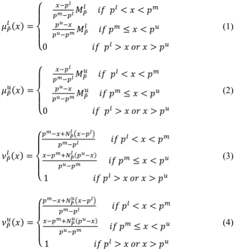
Definition 2. 1. An Interval-valued Pythagorean

triangular fuzzy number _{= 〈 , , , ,} 〉 is

an extension of Interval-valued Pythagorean fuzzy number whose interval-valued membership and non-membership functions are represented as follows:

=

! < <

#

# ! ≤ <

0 ! > '( >

(1)

=

! < <

#

# ! ≤ <

0 ! > '( >

(2)

) =

*+

! < < *+,- #

# ! ≤ <

1 ! > '( >

(3)

) =

*+_,-#

! < < *+_,-# #

# ! ≤ <

1 ! > '( >

(4)

respectively, as depicted in Figure 1.

The values _{= ,} and _{= ,} represent the bound of the maximum degree of membership and the minimum degree of non-membership, respectively, in a way that they satisfy the following conditions:

⊆ 00,11; ⊆ 00,11; 0 ≤ 3+ 3 ≤ 1 and , , ∈ 9

Definition 2. 2. Let _: and ₃ be two IVPTFNs and ; ≥ 0, then their arithmetical operations are defined by Equations (5) to (8); which can make sure that the operational outcomes are also in form of IVPTFNs. Definition 2. 3. let _{; = = 1,2} be two IVPTFNs, then the Hamming distance between _: and ₃ can be defined by Equation (9).

Definition 2. 4. let _{?; @ = 1,2, … , B} be a collection of IVPTFNs, then the function _{CD EFGHI: Ω}L_{→ Ω is} known as an interval-valued Pythagorean triangular fuzzy weighted averaging operator and is expressed in Equation (10), where _N? is the weight of _?, _{N? ∈ 00,11} and ∑L?P:N? = 1.

2. 2. Cut Sets of IVPTFNs

Definition 2. 5. A _{Q, R} -cut set of an IVPTFN is

defined as _{Q,R= S | ≥ Q, ) ≤ RU}, where _{0 ≤}

Q ≤ , _{≤ R ≤ 1} and _{0 ≤ Q}V_{+ R}V_{≤ W.}

Definition 2. 6.A _X -cut set of an IVPTFN is composed

of two crisp subsets, which is defined as _{Q =}

Y | ≥ Z[ and _{Q = S | ≥ ZU}, where _{0 ≤ Z ≤}

and _{0 ≤ Z ≤} , respectively. Then _Q and _Q are closed intervals, which are denoted by:

Q= \Q] , Q^_ = ` + _a Q

,- , +

#_Q

a_,- b , 0 ≤ Q ≤

(11)

Q = \ Q] , Q^_ = ` + _a Q

,-# , + #_Q

a_,-# b , 0 ≤ Q ≤

(12)

Definition 2. 7. A _R -cut set of an IVPTFN is composed of two crisp subset, which are defined as _R=

Y |) ≤ R[ and _{R = S |) ≤ RU}, where _≤

R ≤ 1 and _{≤ R ≤ 1} ,respectively. Then _R and _R are closed intervals, which are denoted by:

R= \ R] , R^_ = `: R * R +

,-: +_,- ,

: R * R +_,- #

: +_,- b , ≤ R ≤ 1

(13)

R = \ R] , R^_ = `: R * R +,-#

: +_,-# , : R * R + ,-# #

: +_,-# b , ≤ R ≤ 1

(14)

:⨁ 3= 〈0 :+ 3, : + 3, :+

31, def _gh

3

+ f _ih3− f _gh3f _ih3, ef _gh3+ f _ih3− f _gh3f _ih3k , _{g i}, _{g i} 〉 (5)

:⨂ 3= 〈0 : 3, : 3, : 31, g i, g i , def gh

3

+ f _ih3− f _gh3f _ih3, ef _gh3+ f _ih3− f _gh3f _ih3k〉

(6)

; := 〈0; :, ; :, ; :1, mn1 − o1 − f gh

3

pq, n1 − o1 − f _gh3pqr , \ _g q, _g q_〉 , ; ≥ 0 (7)

: q= 〈\ :q, : q, :q_ , \ g

q

, _g q_ , mn1 − o1 − f _gh3pq, n1 − o1 − f _gh3pqr〉 (8)

s : , 3 =:_t\uf g

3

− _g3h :− f i

3

− _i3h 3u + uf g

3₋

g

3

h :− f i

3₋

i

3

h 3u + uf g

3

− _g3h : −

f _i3− _i3h 3u + uf g

3₋

g

3

h : − f i

3₋

i

3

h 3u + uf g

3

− _g3h : − f i

3

− _i3h 3u +

uf _g3− _g3h :− f i

3₋

i

3

h 3u_

(9)

CD EFGHI :, 3, … , L = N: :⊕ N3 3⊕ … ⊕ NL L=

〈∑ ?

L

?P: N?, ∑L?P: ? N?, ∑L?P: ?N? mn1 − ∏ o1 − f - xh

3

pIx

L

?P: , n1 − ∏ o1 − f -xh

3

pIx

L

?P: r

\∏

-x

Ix

L

?P: , ∏ -x

Ix

L

?P: _

3.POSSIBILITY EXPECTED VALUE AND VARIANCE OF IVPTFNs

In this section, based on the basic concepts and definitions used in possibility theory, the possibility expected value and variance of IVPTFNs are defined.

3. 1. The Possibility Expected Value of IVPTFNs

Definition 3. 1. Let be an IVPTFN. With respect to Definition2.6, the lower and upper possibilistic expected values of membership function for are explained in the following, respectively.

yz = y Q = { Q |o + _a Q

,- p +

a

,-}

o + _a #Q

,- p~ •Q =

: t

3

+ 4 +

(15)

yz = y Q = { Q |o + _a Q

,-# p +

a,-#

}

o + _a #Q

,-# p~ •Q =

: t

3

+ 4 +

(16)

Definition 3. 2. Let be an IVPTFN. According to Definition2.7, the lower and upper possibilistic expected values of non-membership function for are respectively defined as follows:

y• = y R = { R |o: R _{: +}* R +

,-,- p +

: +

,-o: R * R +,- #

: +_,- p~ •R = :

t 1 − f +

4 + + 2 + + h

(17)

y• = y R = { R |o: R * R +

,-#

: +_,-# p +

: +_,-#

o: R * R +,-# #

: +_,-# p~ •R =:_t 1 − f +

4 + + 2 + + h

(18)

3. 2. The Possibility Variance of IVPTFNs

Definition 3. 3. Let be an IVPTFN. According to Definition2.6, the lower and upper possibilistic variance of membership function for are respectively defined as follows:

D‚(z = D‚( Q =:₃{ Q |o + _a Q

,- p −

a

,-}

o + _a #Q

,- p~

V

•Q =_3ƒ: 3 − 3

(19)

D‚(z = D‚( Q =:₃{ Q |o + _a Q

,-# p −

a_,-#

}

o + _a #Q

,-# p~

V

•Q =_3ƒ: 3 − 3

(20)

Definition 3. 4. Let be an IVPTFN. According to Definition2.7, the lower and upper possibilistic variance of non-membership function for are respectively defined as follows:

D‚(• = D‚( R =:₃{ R |o: R _{: +}* R +

,-,- p −

: +

,-o: R * R +,- #

: +_,- p~ V

•R =_3ƒ: 1 − +

3 − 3

(21)

D‚(• = D‚( R = :

3{ R |o

: R * R +_,-#

: +_,-# p +

: +_,-#

o: R * R +,-# #

: +_,-# p~

V

•R =_3ƒ: 1 − +

3 − 3

(22)

4. NOVEL IVPTF-MAGDM METHOD WITHOUT AGGREGATION

This section presents two new developed forms of MABAC technique to solve the MAGDM problem in IVPTF environment, one is applied to compute the weights of DMs, while the other one is employed to rank the preference order of each alternative. Let _{… =} S…:, …3, … , … U be a discrete set of _{† † ≥ 2} feasible alternatives and _{‡ = S‡:, ‡3, … , ‡L}U be a finit set of _B

B ≥ 2 criteria. Let _{yˆ = S‰ˆ:, ‰ˆ3, … , ‰ˆŠU} be a group of DMs, and let _{; = ;:, ;3, … , ;Š} be the weight vector of DMs, where _{0 ≤ ;‹≤ 1} and _∑Š _;‹

‹P: = 1. We denote the weight vector of criteria for each DM by _N‹₌

N:‹_{, N3}‹_{, … , NL}‹ _{‹ = 1,2, … , Œ , where N}‹ _{is a} normalized vector of attribute relative importance weights satisfying the conditions _∑L _N•‹ ₌

•P: 1 and N•‹≥ 0.

In practical situations of MAGDM, DM and attribute weighting information can be known in advance. In this paper, we suppose that the attribute weights are known precisely, but the DMs’ weighting information is completely unknown. The decision maker _‹ employs the IVPTFN _Ž•‹ _{to show the criterion value of …}

Ž while considering the criterion _‡•. Hence, it is possible to explain the MAGDM problem with IVPTFNs concisely in IVPTF decision matrix as presented in the following:

‹₌

Ž•‹ _×L, ‹ = 1,2, … , Œ (23)

determine the weights of DMs based on IVPTFN. The following presents the basic steps:

i

Construct the weighted IVPTF decision matrix ‘-‹_{= ‘}

-Ž• ‹

×Lfor each DM by appling the

multiplication by a constant operator on ‹₌ Ž•‹ _×Land N‹= N:‹, N3‹, … , NL‹ by:

‘-‹_{= N}

•‹ Ž•‹ _×L=

’ “ “ “ “ ”

\N•‹ Ž•‹, N•‹ Ž•‹ , N•‹ Ž•‹ _ ,

mn1 − |1 − o

•–‹p

3 ~

I–‹

, n1 − |1 − o

•–‹p

3 ~

I–‹

r ,

do _•–‹p

I–‹

, o _•–‹p

I–‹

k

— ˜ ˜ ˜ ˜ ™

×L

(24)

(ii)

Finding a boarder approximation area of each element of a decision matrix in order to distinguish the ideal and the anti-ideal solutions. For this purpose, the CD EFGšI operator is used. The following is therefore presented:

›Ž•= ∏ ‘-Ž•‹

g œ

Š

•P: = ; = 1,2, … , † ž = 1,2, … , B

〈

d∏ fŸŽ•‹h

g œ

Š

•P: , ∏ fŸŽ•‹ h

g œ

Š

•P: , ∏ fŸŽ•‹ h

g œ

Š

•P: k

∏ o -_‘-_•–‹p

g œ

Š

•P: , ∏ o -‘-_•–‹p

g œ

Š

•P: ¡ ,

¢n1 − ∏ |1 − o -_‘-_•–‹p

3 ~

g œ

Š

•P: , n1 − ∏ |1 − o -‘-_•–‹p

3 ~

g œ

Š

•P: £

〉

(25)

by using the values of _{›Ž•, = 1,2, … , † ž =} 1,2, … , B , the matrix _› which denotes the area of border approximation can be obtained as the following format:

› = ›Ž• _×L (26)

(iii)

In order to compute the relative distance of each element of weighted IVPTF decision matrix from the border approximation, the Hamming distance operator of IVPTFNs is employed and the distance matrix _D‹ _is constructed as follows:

D‹_{= s}

Ž•‹ _×L (27)

sŽ•‹= s ‘-Ž•‹ , ›Ž• =:_t`¥o _‘-_•–‹3− _‘ -•– ‹3p Ÿ_Ž•‹ −

f _¦•–3− _¦•–3h §Ž•¥ + ¥o ‘-_•–‹3− _‘ -•– ‹3p Ÿ_Ž•‹ −

f _¦•–3− _¦•–3h §Ž•¥ + ¥o ‘-_•–‹3− _‘ -•–

‹3p Ÿ_Ž•‹ −

f _¦•–3− _¦•–3h §Ž•¥ + ¥o ‘-_•–‹3− _‘ -•–‹

3 p ŸŽ•‹ − f _¦•–3− _¦•–3h §Ž•¥ + ¥o ‘-_•–‹3− _‘

-•–‹

3_{p Ÿ} Ž• ‹ ₋

f _¦•–3− _¦•–3h §Ž•¥ + ¥o ‘-_•–‹3− _‘ -•–

‹3p Ÿ_Ž•‹ −

f _¦•–3− _¦•–3h §Ž•¥b

(28)

Obviously, the element _‘-_Ž•‹ _{will be a part of to the border} approximation area, the area which contains the ideal

solutions, if _sŽ•‹_{= 0. In the same way, ‘} -Ž•

‹ _{will belong to} the upper approximation area or the lower approximation area which contain the anti-ideal solutions when _sŽ•‹ _{≥ 0.}

(iv)

Determine the weight of each DMs based on the distance matrices _D‹ _{‹ = 1,2, … , Œ . In order for matrix} ‘-‹ _{and consequently ‹}©ª _{DM to be chosen as the most} important one, it is necessary for it to have as many elements as possible belonging to the border approximation area. As a result, the following is used to compute the weight of each DM:

;‹= 1 ∑ ∑ «•–

‹ ¬ –-g •-g

∑œ‹-g∑•-g∑¬–-g«•–‹

® (29)

(v)

Normalize the weight of each DM such that _;‹≥ 0, ∑Š ;‹

‹P: = 1.

;‹= ;‹ _∑Š _;‹ ‹P:

¯ (30)

4. 2. New Extended Version of MABAC Method based on Possibility Theory for Ranking the Preference Order of Alternative In this subsection, a modified version of MABAC method is proposed based on possibility theory. As is known, the decision information may be lost by applying the aggregation operators. In order to avoid information loss, the proposed approach has no aggregating process. A MAGDM model can be described in detail by means of the following steps:

I. Based on the weight vector of DMs _{;‹ , ‹ =} 1,2, … , Œ , _;‹ is assigned to individual decision matrix ‘-Ž•‹ as Equation (31).

II. Different attributes with various amounts own various dimensions. To diminish the consequence of this sort of inconvenience, various attribute scales ought to be changed to a scale that is comparable. Equation (32) presents the normalizing relations, where, _°‹_{± =} max

Ž °Ž•

‹ _{and °} ŽL ‹ _{= min}

Ž °Ž•

‹ _{. Based on the values} ´-µ¶‹

····, = 1,2,…,† ž = 1,2,… ,B , the normalized weighted decision matrix _´- ···· = f´-‹

µ¶ ‹ ····h

×Lcan be formed. III. The possibilistic expected value of the _´-µ¶····‹ _are computed according to definition 3.1 and definition 3.2, as Equation (33); where yzf´-····h =µ¶‹ :_to _´-···_¸¹‹p

3 o°··· +µ¶‹

4°···µ¶‹ + °···µ¶‹ p, yzf´-····h = µ¶‹ :_to _´-···_¸¹‹p

3

o°··· + 4°µ¶‹ ··· + °µ¶‹ ···pµ¶‹ , y•f´-····h =µ¶‹ :_t o1 − _´-···_¸¹‹p | ···_´-¸¹‹ o°··· + 4°µ¶‹ ···µ¶‹ + °···µ¶‹ p +

2 o°··· + °µ¶‹ ···µ¶‹ + °···µ¶‹ p~ and y•f´-····h =µ¶‹ :_to1 −

´-¸¹‹

···p | _´-···_¸¹‹ o°··· + 4°µ¶‹ ···‹µ¶ + °···µ¶‹ p + 2 o°··· + °µ¶‹ ···µ¶‹ +

(31)

´-‹_{= ;}

‹‘-Ž•‹ _×L

= º\;‹ŸŽ•‹ , ;‹ŸŽ•‹ , ;‹ŸŽ•‹ _ , mn1 − |1 − o ‘-_•–‹p

3 ~

q‹

, n1 − |1 − o _‘

-•– ‹p

3 ~

q‹

r , do _‘

-•– ‹p

q‹

, o _‘

-•– ‹p

q‹

k» ×L

(32)

´-µ¶‹ ···· = |d

°_•–‹ °‹_•¬ °‹¼½ °‹•¬,

°_•–‹ °‹_•¬ °‹¼½ °‹•¬,

°_•–‹ # °‹_•¬

°‹¼½ °‹•¬k , ` ´-•–‹, ´-•–‹b , ` ´-•–‹, ´-•–‹b~ ; ž ∈ ›enefit

|d°‹¼½ °•–‹ #

°‹¼½ °‹•¬,

°‹¼½ °•–‹

°‹¼½ °‹•¬,

°‹¼½ °•–‹

°‹¼½ °‹•¬k , ` ´-•–‹, ´-•–‹b , ` ´-•–‹, ´-•–‹b~ ; ž ∈ Áost

(33)

y f´-µ¶····h = \yz‹ _f´-µ¶····h,y•‹ _f´-µ¶····h_ = `\y‹ _zf´-µ¶····h,yz‹ _f´-µ¶····h_,\y•‹ _f´-µ¶····h,y‹ _{• f´-µ¶}····h_b‹

IV. The possibilistic variance of the IVPTFN _´-····_µ¶‹ _are computed according to definition 3.3 and definition 3.4, as

D‚(f´-····h = \D‚(µ¶‹ zf´-····h,D‚(µ¶‹ •f´-····h_ =µ¶‹

`\D‚(zf´-····h,D‚(µ¶‹ z f´-····h_,\D‚(‹µ¶ •f´-····h ,D‚(µ¶‹ • f´-····h_bµ¶‹

(34)

where _D‚(zf´-····h =_µ¶‹ : 3ƒo ´-···p¸¹‹

3

f°··· − °µ¶‹ ···hµ¶‹ 3

,

D‚(z f´-µ¶····h =‹ _3ƒ: o

´-¸¹ ‹

···p3f°µ¶··· − °µ¶‹ ···h‹ 3_{, D‚(•f´-µ¶}····h =‹ :

3ƒ o1 − ´-···p o¸¹‹ ´-···¸¹‹+ 3p f°µ¶

‹

··· − °···hµ¶‹ 3

and

D‚(• f´-····h =µ¶‹ _3ƒ: o1 − ···p o_´-¸¹‹ _´-···_¸¹‹+ 3p f°··· − °µ¶‹ ···hµ¶‹ 3

. Accordingly, the possibilistic standard deviation of _´-····_µ¶‹_is calculated as

ÄÅf´····h = \ÄÅ-_µ¶‹

zf´····h,ÄÅ-µ¶‹ •f´····h_ =-µ¶‹

deD‚(zf´····h,eD‚(-µ¶‹ z f´····hk,deD‚(-µ¶‹ •f´····h,eD‚(-µ¶‹ • f´····hk¡-µ¶‹

(35)

V. The possibilistic expected value matrix, _Æ‹_{, and the} possibilisti standard deviation matrix, _ÇÈ‹_{, of the} normalized weighted decision matrix _´-···· = f´-‹

µ¶‹ ····h

×Lare constructed as follows:

Æ‹_{= É} Ž• ‹

×L=

f`\ ÉŽ•‹ <sub>:</sub>, ÉŽ•‹ <sub>3</sub>_ , \ ÉŽ•‹ <sub>Ê</sub>, ÉŽ•‹ <sub>ƒ</sub>_bh ×L= f`\y_z f´-····h,yµ¶‹ _z f´-····h_,\y‹µ¶ • f´-····h,yµ¶‹ • f´-····h_bhµ¶‹

×L

‹ = 1,2, … , Œ

(36)

ÇÈ‹_{= ËÌ}

Ž• ‹

×L=

f`\ ËÌŽ•‹ _:, ËÌŽ•‹ ₃_ , \ ËÌŽ•‹ _Ê, ËÌŽ•‹ _ƒ_bh

×L=

f`\ÄÅ_z f´-····h,Äŵ¶‹ _z f´-····h_,\Äŵ¶‹ • f´-····h,Äŵ¶‹ • f´-····h_bhµ¶‹

×L ‹ = 1,2, … , Œ

(37)

VI. The individual possibilistic expected value matrix, Æ‹_{, and possibilistic standard deviation matrix, ÇÈ}‹ _are converted into the group decision form of alternative as follows:

ÆŽ_{= É} ‹• Ž

©×L=

f`\ É‹•Ž _:, É‹•Ž ₃_ , \ É‹•Ž _Ê, É‹•Ž _ƒ_bh ©×L = 1,2, … , †

(38)

ÇÈŽ_{= ËÌ} ‹• Ž

©×L=

f`\ ËÌ‹•Ž _:, ËÌ‹•Ž ₃_ , \ ËÌ‹•Ž _Ê, ËÌ‹•Ž _ƒ_bh ©×L = 1,2, … , †

(39)

where the element _É‹•Ž _{is the element É}

Ž•‹ shown in Æ‹ and similarly, the element _ËÌ‹•Ž _{is is the element ËÌŽ•}‹ _shown in _ÇÈ‹_.

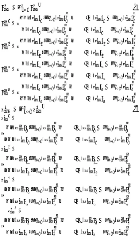
VII. The border approximation area matrix based on the expected and the standard deviation values are defined by Equations (40 and 41).

VIII. Using the Euclidean distance operator, the distances of the candidate alternative from the expected value-based and the standard deviation-value-based border approximation area matrices, _{BÎ and BÏÐ}, are computed to construct the expected value-based distance matrix XŽ₌

‹•Ž _Š×Land the standard deviation -based distance matrix _YŽ_{= Ó}

‹•Ž _Š×Las shown in Equations (42 and 43).

BÎ = o∏ É‹•Ž

g

ÔP: p

©×L= | `∏ É‹• Ž

:

g

ŽP: , ∏ É‹•Ž ₃

g

ŽP: b , `∏ É‹•Ž _Ê

g

ŽP: , ∏ É‹•Ž _ƒ

g

ŽP: b¡~

©×L

(40)

BÏÐ= o∏ ËÌ‹•Ž

g

ÔP: p

©×L= | `∏ ËÌ‹• Ž

:

g

ŽP: , ∏ ËÌ‹•Ž ₃

g

ŽP: b , `∏ ËÌ‹•Ž _Ê

g

ŽP: , ∏ ËÌ‹•Ž _ƒ

g

ŽP: b¡~

©×L

‹•Ž = ∑ƒ?P: ‹•Ž ? (42)

‹•Ž := Õ

−s o É‹•Ž _: , ∏ É‹•Ž _:

g

ŽP: p ! É‹•Ž _:< ∏ É‹•Ž _:

g

ŽP:

s o É‹•Ž _: , ∏ É‹•Ž _:

g

ŽP: p ! É‹•Ž _:> ∏ É‹•Ž _:

g

ŽP:

‹•Ž 3= Õ

−s o É‹•Ž ₃ , ∏ É‹•Ž ₃

g

ŽP: p ! É‹•Ž ₃< ∏ É‹•Ž ₃

g

ŽP:

s o É‹•Ž ₃ , ∏ É‹•Ž ₃

g

ŽP: p ! É‹•Ž ₃> ∏ É‹•Ž ₃

g

ŽP:

‹•Ž Ê= Õ

s o É‹•Ž _Ê , ∏ É‹•Ž _Ê

g

ŽP: p ! É‹•Ž _Ê< ∏ É‹•Ž _Ê

g

ŽP:

−s o É‹•Ž _Ê , ∏ É‹•Ž _Ê

g

ŽP: p ! É‹•Ž _Ê> ∏ É‹•Ž _Ê

g

ŽP:

‹•Ž ƒ= Õ

s o É‹•Ž _ƒ , ∏ É‹•Ž _ƒ

g

ŽP: p ! É‹•Ž _ƒ< ∏ É‹•Ž _ƒ

g

ŽP:

−s o É‹•Ž _ƒ , ∏ É‹•Ž _ƒ

g

ŽP: p ! É‹•Ž _ƒ> ∏ É‹•Ž _ƒ

g

ŽP:

Ó‹•Ž = ∑ƒ?P:Ó‹•Ž ? (43)

Ó‹•Ž :=

Õs o ËÌ‹•

Ž

: , ∏ ËÌ‹•Ž :

g

ŽP: p ! ËÌ‹•Ž _:< ∏ ËÌ‹•Ž _:

g

ŽP:

−s o ËÌ‹•Ž _: , ∏ ËÌ‹•Ž _:

g

ŽP: p ! ËÌ‹•Ž _:> ∏ ËÌ‹•Ž _:

g

ŽP:

Ó‹•Ž 3=

Õs o ËÌ‹•

Ž

3 , ∏ ËÌ‹•Ž 3

g

ŽP: p ! ËÌ‹•Ž ₃< ∏ ËÌ‹•Ž ₃

g

ŽP:

−s o ËÌ‹•Ž ₃ , ∏ ËÌ‹•Ž ₃

g

ŽP: p ! ËÌ‹•Ž ₃> ∏ ËÌ‹•Ž ₃

g

ŽP:

Ó‹•Ž Ê=

Õ−s o ËÌ‹•

Ž

Ê , ∏ ËÌ‹•Ž Ê

g

ŽP: p ! ËÌ‹•Ž _Ê< ∏ ËÌ‹•Ž _Ê

g

ŽP:

s o ËÌ‹•Ž _Ê , ∏ ËÌ‹•Ž _Ê

g

ŽP: p ! ËÌ‹•Ž _Ê> ∏ ËÌ‹•Ž _Ê

g

ŽP:

Ó‹•Ž ƒ=

Õ−s o ËÌ‹•

Ž

ƒ , ∏ ËÌ‹•Ž ƒ

g

ŽP: p ! ËÌ‹•Ž _ƒ< ∏ ËÌ‹•Ž _ƒ

g

ŽP:

s o ËÌ‹•Ž _ƒ , ∏ ËÌ‹•Ž _ƒ

g

ŽP: p ! ËÌ‹•Ž _ƒ> ∏ ËÌ‹•Ž _ƒ

g

ŽP:

IX. In order to evaluate the alternatives, the closeness

coefficient _ℵŽ _{of group decision of each alternative to the} border approximation area is defined as:

ℵŽ_{= × ∑ ∑} ‹•Ž L ŽP: Š

‹P: + 1 − × f ∑Š‹P:∑LŽP:Ó‹•Ž h (44) where, _{0 ≤ × ≤ 1} is the importance coefficient. Value of × can be decided based on the group’s opinion.

X. Closeness coefficients of alternatives are used to rank them. The alternatives are ranked in decreasing order of the closeness coefficient _ℵŽ_{. The bigger values}

5. CASE STUDY

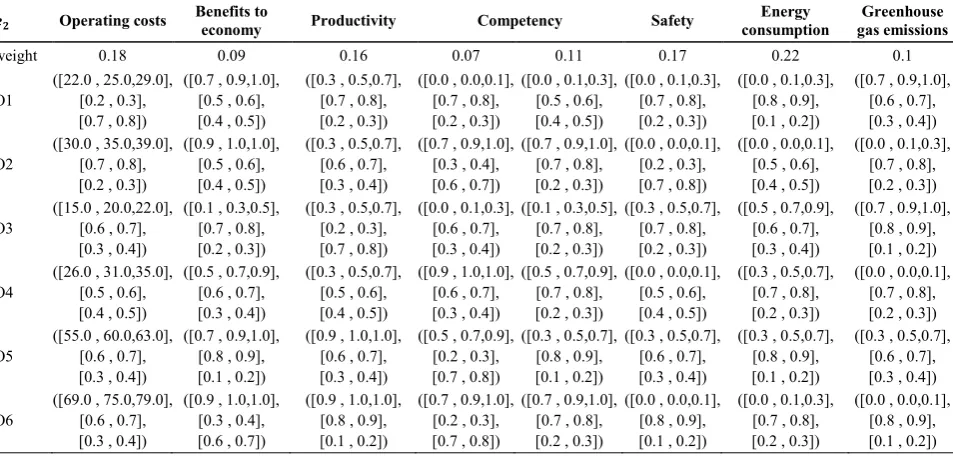
In this section, in order to explain the applicability of the proposed methods in real-world problems, they are used in a real case study of an Iranian transport complex. The company is presented with six alternative marine transport investments, _{… = S…:, …3, …Ê, …ƒ, …Ø, …t}U. Due to the limited investment funds, the company wants to choose the best one of the projects to fund and operate. Their main goal is to improve their position in the market through focusing on issues, such as operating costs _‡: ,

benefits to economy _‡3 , productivity _‡Ê ,

competency _‡ƒ , Safety _‡Ø , Energy consumption _‡t and Greenhouse gas emissions _‡Ù . Due to the competitive environment, the company has reserved the information of candidate projects as confidential.

A committee of three decision makers, _{yˆ =} S‰ˆ:, ‰ˆ3, ‰ˆÊU, with at least 9 years of experience in the marine transport sector is formed to select the best sustainable marine transportation project for investment.

The assessment value of alternatives with respect to criteria and the information about the attribute weights are directly provided by experts’ judgments as shown in Tables 1 to 3. By utilizing the method proposed in

TABLE 1. IVPTFN decision matrix given by expert _‰ˆ:

ÚˆW Operating costs Benefits to _economy Productivity Competency Safety Energy consumption _{gas emissions} Greenhouse

weight 0.26 0.14 0.15 0.09 0.16 0.1 0.1

O1

([20.0,27.0,29.0], [0.3,0.4], [0.6 , 0.7])

([0.3,0.5,0.7], [0.5 , 0.6], [0.4 , 0.5])

([0.7, 0.9,1.0], [0.7 , 0.8], [0.2 , 0.3])

([0.7 , 0.9,1.0], [0.6 , 0.7], [0.3 , 0.4])

([0.1 , 0.3,0.5], [0.7 , 0.8], [0.2 , 0.3])

([0.7 , 0.9,1.0], [0.8 , 0.9], [0.1 , 0.2])

([0.7 , 0.9,1.0], [0.6 , 0.7], [0.3 , 0.4])

O2

([33.0,35.0,40.0], [0.7 , 0.8], [0.2 , 0.3])

([0.3 , 0.5,0.7], [0.7 , 0.8], [0.2 , 0.3])

([0.3 , 0.5,0.7], [0.6 , 0.7], [0.3 , 0.4])

([0.9 , 1.0,1.0], [0.7 , 0.8], [0.2 , 0.3])

([0.7 , 0.9,1.0], [0.7 , 0.8], [0.2 , 0.3])

([0.0 , 0.1,0.3], [0.8 , 0.9], [0.1 , 0.2])

([0.0 , 0.1,0.3], [0.7 , 0.8], [0.2 , 0.3])

O3

([11.0 , 20.0,23.0], [0.6 , 0.7], [0.3 , 0.4])

([0.7 , 0.9,1.0], [0.3 , 0.4], [0.6 , 0.7])

([0.3 , 0.5,0.7], [0.8 , 0.9], [0.1 , 0.2])

([0.0 , 0.1,0.3], [0.7 , 0.8], [0.2 , 0.3])

([0.0 , 0.1,0.3], [0.8 , 0.9], [0.1 , 0.2])

([0.5 , 0.7,0.9], [0.5 , 0.6], [0.4 , 0.5])

([0.7 , 0.9,1.0], [0.8 , 0.9], [0.1 , 0.2])

O4

([24.0 , 29.0,33.0], [0.2 , 0.3], [0.7 , 0.8])

([0.7 , 0.9,1.0], [0.7 , 0.8], [0.2 , 0.3])

([0.5 , 0.7,0.9], [0.5 , 0.6], [0.4 , 0.5])

([0.9 , 1.0,1.0], [0.8 , 0.9], [0.1 , 0.2])

([0.7 , 0.9,1.0], [0.6 , 0.7], [0.3 , 0.4])

([0.0 , 0.1,0.3], [0.7 , 0.8], [0.2 , 0.3])

([0.0 , 0.0,0.1], [0.7 , 0.8], [0.2 , 0.3])

O5 ([58.0 , 62.0,65.0],[0.5 , _{0.6],[0.4 , 0.5])}

([0.5 , 0.7,0.9], [0.1 , 0.2], [0.8 , 0.9])

([0.0 , 0.1,0.3], [0.6 , 0.7], [0.3 , 0.4])

([0.0 , 0.1,0.3], [0.6 , 0.7], [0.3 , 0.4])

([0.3 , 0.5,0.7], [0.8 , 0.9], [0.1 , 0.2])

([0.7 , 0.9,1.0],[0.3, 0.4],[0.6 , 0.7])

([0.3 , 0.5,0.7], [0.6 , 0.7], [0.3 , 0.4])

O6

([72.0 , 78.0,85.0], [0.3 , 0.4], [0.6 , 0.7])

([0.5 , 0.7,0.9], [0.7 , 0.8], [0.2 , 0.3])

([0.1 , 0.3,0.5], [0.8 , 0.9], [0.1 , 0.2])

([0.7 , 0.9,1.0], [0.7 , 0.8], [0.2 , 0.3])

([0.7 , 0.9,1.0], [0.6 , 0.7], [0.3 , 0.4])

([0.0 , 0.1,0.3], [0.3 , 0.4], [0.6 , 0.7])

TABLE 2. IVPTFN decision matrix given by expert _‰ˆ3

ÚˆV Operating costs Benefits to _economy Productivity Competency Safety _consumption Energy _{gas emissions} Greenhouse

weight 0.3 0.18 0.28 0.1 0.05 0.07 0.02 0.1

O1

([17.0,22.0,25.0], [0.7 , 0.8], [0.2 , 0.3])

([0.9,1.0,1.0], [0.7 , 0.8], [0.2 , 0.3])

([0.7,0.9,1.0], [0.6 , 0.7], [0.3 , 0.4])

([0.1 , 0.3,0.5], [0.2 , 0.3], [0.7 , 0.8])

([0.3 , 0.5,0.7], [0.7 , 0.8], [0.2 , 0.3])

([0.3 , 0.5,0.7], [0.7 , 0.8], [0.2 , 0.3])

([0.3 , 0.5,0.7], [0.8 , 0.9], [0.1 , 0.2])

([0.7 , 0.9,1.0], [0.6 , 0.7], [0.3 , 0.4])

O2

([36.0,40.0,42.0], [0.7 , 0.8], [0.2 , 0.3])

([0.5 , 0.7,0.9], [0.7 , 0.8], [0.2 , 0.3])

([0.0 , 0.1,0.3], [0.6 , 0.7], [0.3 , 0.4])

([0.5 , 0.7,0.9], [0.6 , 0.7], [0.3 , 0.4])

([0.7 , 0.9,1.0], [0.8 , 0.9], [0.1 , 0.2])

([0.1 , 0.3,0.5], [0.7 , 0.8], [0.2 , 0.3])

([0.1 , 0.3,0.5], [0.6 , 0.7], [0.3 , 0.4])

([0.0 , 0.1,0.3], [0.7 , 0.8], [0.2 , 0.3])

O3 ([10.0,16.0,24.0],[0.8 , 0.9], [0.1 , 0.2])

([0.3 , 0.5,0.7], [0.7 , 0.8], [0.2 , 0.3])

([0.5 , 0.7,0.9], [0.5 , 0.6], [0.4 , 0.5])

([0.0 , 0.1,0.3], [0.7 , 0.8], [0.2 , 0.3])

([0.1 , 0.3,0.5], [0.6 , 0.7], [0.3 , 0.4])

([0.1 , 0.3,0.5], [0.2 , 0.3], [0.7 , 0.8])

([0.5 , 0.7,0.9], [0.6 , 0.7], [0.3 , 0.4])

([0.7 , 0.9,1.0], [0.8 , 0.9], [0.1 , 0.2])

O4 ([26.0,30.0,37.0],[0.6 , 0.7], [0.3 , 0.4])

([0.0 , 0.1,0.3], [0.7 , 0.8], [0.2 , 0.3])

([0.1 , 0.3,0.5], [0.7 , 0.8], [0.2 , 0.3])

([0.5 , 0.7,0.9], [0.7 , 0.8], [0.2 , 0.3])

([0.7 , 0.9,1.0], [0.8 , 0.9], [0.1 , 0.2])

([0.1 , 0.3,0.5], [0.7 , 0.8], [0.2 , 0.3])

([0.1 , 0.3,0.5], [0.5 , 0.6], [0.4 , 0.5])

([0.0 , 0.0,0.1], [0.7 , 0.8], [0.2 , 0.3])

O5 ([53.0,57.0,61.0],[0.7 , 0.8], [0.2 , 0.3])

([0.5 , 0.7,0.9], [0.7 , 0.8], [0.2 , 0.3])

([0.3 , 0.5,0.7], [0.3 , 0.4], [0.6 , 0.7])

([0.7 , 0.9,1.0], [0.7 , 0.8], [0.2 , 0.3])

([0.3 , 0.5,0.7], [0.6 , 0.7], [0.3 , 0.4])

([0.9 , 1.0,1.0], [0.8 , 0.9], [0.1 , 0.2])

([0.5 , 0.7,0.9], [0.7 , 0.8], [0.2 , 0.3])

([0.3 , 0.5,0.7], [0.6 , 0.7], [0.3 , 0.4])

O6 ([75.0,80.0,84.0],[0.3 , 0.4], [0.6 , 0.7])

([0.7 , 0.9,1.0], [0.7 , 0.8], [0.2 , 0.3])

([0.7 , 0.9,1.0], [0.2 , 0.3], [0.7 , 0.8])

([0.9 , 1.0,1.0],[0.6 , 0.7],[0.3 , 0.4])

([0.7 , 0.9,1.0], [0.7 , 0.8], [0.2 , 0.3])

([0.5 , 0.7,0.9], [0.6 , 0.7], [0.3 , 0.4])

([0.1 , 0.3,0.5], [0.5 , 0.6], [0.4 , 0.5])

([0.0 , 0.0,0.1], [0.8 , 0.9], [0.1 , 0.2])

TABLE 3. IVPTFN decision matrix given by expert _‰ˆÊ

ÚˆV Operating costs Benefits to _economy Productivity Competency Safety _consumption Energy _{gas emissions} Greenhouse

weight 0.18 0.09 0.16 0.07 0.11 0.17 0.22 0.1

O1

([22.0 , 25.0,29.0], [0.2 , 0.3], [0.7 , 0.8])

([0.7 , 0.9,1.0], [0.5 , 0.6], [0.4 , 0.5])

([0.3 , 0.5,0.7], [0.7 , 0.8], [0.2 , 0.3])

([0.0 , 0.0,0.1], [0.7 , 0.8], [0.2 , 0.3])

([0.0 , 0.1,0.3], [0.5 , 0.6], [0.4 , 0.5])

([0.0 , 0.1,0.3], [0.7 , 0.8], [0.2 , 0.3])

([0.0 , 0.1,0.3], [0.8 , 0.9], [0.1 , 0.2])

([0.7 , 0.9,1.0], [0.6 , 0.7], [0.3 , 0.4])

O2

([30.0 , 35.0,39.0], [0.7 , 0.8], [0.2 , 0.3])

([0.9 , 1.0,1.0], [0.5 , 0.6], [0.4 , 0.5])

([0.3 , 0.5,0.7], [0.6 , 0.7], [0.3 , 0.4])

([0.7 , 0.9,1.0], [0.3 , 0.4], [0.6 , 0.7])

([0.7 , 0.9,1.0], [0.7 , 0.8], [0.2 , 0.3])

([0.0 , 0.0,0.1], [0.2 , 0.3], [0.7 , 0.8])

([0.0 , 0.0,0.1], [0.5 , 0.6], [0.4 , 0.5])

([0.0 , 0.1,0.3], [0.7 , 0.8], [0.2 , 0.3])

O3

([15.0 , 20.0,22.0], [0.6 , 0.7], [0.3 , 0.4])

([0.1 , 0.3,0.5], [0.7 , 0.8], [0.2 , 0.3])

([0.3 , 0.5,0.7], [0.2 , 0.3], [0.7 , 0.8])

([0.0 , 0.1,0.3], [0.6 , 0.7], [0.3 , 0.4])

([0.1 , 0.3,0.5], [0.7 , 0.8], [0.2 , 0.3])

([0.3 , 0.5,0.7], [0.7 , 0.8], [0.2 , 0.3])

([0.5 , 0.7,0.9], [0.6 , 0.7], [0.3 , 0.4])

([0.7 , 0.9,1.0], [0.8 , 0.9], [0.1 , 0.2])

O4

([26.0 , 31.0,35.0], [0.5 , 0.6], [0.4 , 0.5])

([0.5 , 0.7,0.9], [0.6 , 0.7], [0.3 , 0.4])

([0.3 , 0.5,0.7], [0.5 , 0.6], [0.4 , 0.5])

([0.9 , 1.0,1.0], [0.6 , 0.7], [0.3 , 0.4])

([0.5 , 0.7,0.9], [0.7 , 0.8], [0.2 , 0.3])

([0.0 , 0.0,0.1], [0.5 , 0.6], [0.4 , 0.5])

([0.3 , 0.5,0.7], [0.7 , 0.8], [0.2 , 0.3])

([0.0 , 0.0,0.1], [0.7 , 0.8], [0.2 , 0.3])

O5

([55.0 , 60.0,63.0], [0.6 , 0.7], [0.3 , 0.4])

([0.7 , 0.9,1.0], [0.8 , 0.9], [0.1 , 0.2])

([0.9 , 1.0,1.0], [0.6 , 0.7], [0.3 , 0.4])

([0.5 , 0.7,0.9], [0.2 , 0.3], [0.7 , 0.8])

([0.3 , 0.5,0.7], [0.8 , 0.9], [0.1 , 0.2])

([0.3 , 0.5,0.7], [0.6 , 0.7], [0.3 , 0.4])

([0.3 , 0.5,0.7], [0.8 , 0.9], [0.1 , 0.2])

([0.3 , 0.5,0.7], [0.6 , 0.7], [0.3 , 0.4])

O6

([69.0 , 75.0,79.0], [0.6 , 0.7], [0.3 , 0.4])

([0.9 , 1.0,1.0], [0.3 , 0.4], [0.6 , 0.7])

([0.9 , 1.0,1.0], [0.8 , 0.9], [0.1 , 0.2])

([0.7 , 0.9,1.0], [0.2 , 0.3], [0.7 , 0.8])

([0.7 , 0.9,1.0], [0.7 , 0.8], [0.2 , 0.3])

([0.0 , 0.0,0.1], [0.8 , 0.9], [0.1 , 0.2])

([0.0 , 0.1,0.3], [0.7 , 0.8], [0.2 , 0.3])

([0.0 , 0.0,0.1], [0.8 , 0.9], [0.1 , 0.2])

subsection 4.1, the weight vector of experts can be obtained by:

;:= 0.4029, ;3= 0.2167, ;Ê= 0.3804 (45) The decision procedure for the selection of appropriate sustainable marine transportation project can be detailed by the following steps, proposed in subsection 4.2. The ranking order of all the alternatives is obtained by (_{× =} 0.5):

…Ê≻ …Ø≻ …:≻ …ƒ≻ …t≻ …3 (46)

In order to explore the robustness of the model, parameter × is changed. The results show that the ranking stays robust.

6. CONCLUSION

an uncertain environment. Therefore, to better model, such information in decision problems, the notion of IVPTFNs is defined and their operational rules are proposed. To address group decision making with preference values that can be best expressed in the form of IVPTFNs and have the unknown DMs’ weights, this paper offered a new approach of decision making based on the possibility theory, employing the possibility expected value and variance of IVPTFNs. The proposed method is straightforward, the alternative that possesses high possibilistic mean value in addition to low possibilistic standard deviation will be selected. Moreover, the presented method has no loss of information because the aggregation(s) in a decision process is avoided. In this method, the distance measure between the individual and the border approximation area matrix was used to objectively determine the DMs’ weights. The proposed method is tested in a case study of the Iranian transport complex. The results show that this method is promising. Furthermore, the method can be used to assess the sustainability of the company’s transport projects. For further research, extending the developed method to support a higher degree of uncertainty in the model will be an interesting idea. For instance, definition and application of the interval-valued Pythagorean trapezoidal fuzzy numbers will also allow incorporating additional knowledge about uncertainty in the decision-making process.

7. REFERENCES

1. Yager, R. R., “Pythagorean fuzzy subsets”, In 2013 Joint IFSA World Congress and NAFIPS Annual Meeting (IFSA/NAFIPS), (2013), 57–61.

2. Atanassov, K. T., “Intuitionistic fuzzy sets”, Fuzzy Sets and Systems, Vol. 20, No. 1, (1986), 87–96.

3. Zhang, X., “Multicriteria Pythagorean fuzzy decision analysis: A hierarchical QUALIFLEX approach with the closeness index-based ranking methods”, Information Sciences, Vol. 330, (2016), 104–124.

4. Vahdani, B., Salimi, M., and Mousavi, S.M., “A New Compromise Decision-making Model based on TOPSIS and VIKOR for Solving Multi-objective Large-scale Programming Problems with a Block Angular Structure under Uncertainty”, International Journal of Engineering - Transactions B: Applications, Vol. 27, No. 11, (2014), 1673–1680.

5. Garg, H., “A novel accuracy function under interval-valued Pythagorean fuzzy environment for solving multicriteria decision making problem”, Journal of Intelligent & Fuzzy Systems, Vol. 31, No. 1, (2016), 529–540.

6. Ma, Z. and Xu, Z., “Symmetric Pythagorean Fuzzy Weighted Geometric/Averaging Operators and Their Application in Multicriteria Decision-Making Problems”, International Journal of Intelligent Systems, Vol. 31, No. 12, (2016), 1198– 1219.

7. Ren, P., Xu, Z., and Gou, X., “Pythagorean fuzzy TODIM approach to multi-criteria decision making”, Applied Soft Computing, Vol. 42, (2016), 246–259.

8. Zeng, S., Chen, J., and Li, X., “A Hybrid Method for Pythagorean Fuzzy Multiple-Criteria Decision Making”, International Journal of Information Technology & Decision Making, Vol. 15, No. 02, (2016), 403–422.

9. Li, H., Cao, Y., Su, L., and Xia, Q., “An Interval Pythagorean Fuzzy Multi-criteria Decision Making Method Based on Similarity Measures and Connection Numbers”, Information, Vol. 10, No. 2, (2019), 80.

10. Dorfeshan, Y., and Mousavi, S.M., “A group TOPSIS-COPRAS methodology with Pythagorean fuzzy sets considering weights of experts for project critical path problem”, Journal of Intelligent & Fuzzy Systems, Vol. 36, No. 2, (2019), 1375–1387. 11. Dorfeshan, Y., Mousavi, S.M., Vahdani, B., and Mohagheghi, V.,

“Solving Critical Path Problem in Project Network by a New Enhanced Multi-objective Optimization of Simple Ratio Analysis Approach with Interval Type-2 Fuzzy Sets”, International Journal of Engineering - Transactions C: Aspects, Vol. 30, No. 9, (2017), 1352–1361.

12. Peng, X. and Yang, Y., “Pythagorean Fuzzy Choquet Integral Based MABAC Method for Multiple Attribute Group Decision Making”, International Journal of Intelligent Systems, Vol. 31, No. 10, (2016), 989–1020.

13. Mousavi, S. M., “Solving New Product Selection Problem by a New Hierarchical Group Decision-making Approach with Hesitant Fuzzy Setting”, International Journal of Engineering - Transactions B: Applications, Vol. 30, No. 5, (2017), 729–738. 14. Shakeel, M., bdullah, S., Shahzad, M., and Siddiqui, N., “Geometric aggregation operators with interval-valued Pythagorean trapezoidal fuzzy numbers based on Einstein operations and their application in group decision making”, International Journal of Machine Learning and Cybernetics, (2019), 1–20.

15. Garg, H., “A New Generalized Pythagorean Fuzzy Information Aggregation Using Einstein Operations and Its Application to Decision Making”, International Journal of Intelligent Systems, Vol. 31, No. 9, (2016), 886–920.

16. Yu, C., Shao, Y., Wang, K., and Zhang, L., “A group decision making sustainable supplier selection approach using extended TOPSIS under interval-valued Pythagorean fuzzy environment”, Expert Systems with Applications, Vol. 121, (2019), 1–17. 17. Mohagheghi, V., Mousavi, S. M., and Vahdani, B., “Enhancing

decision-making flexibility by introducing a new last aggregation evaluating approach based on multi-criteria group decision making and Pythagorean fuzzy sets”, Applied Soft Computing, Vol. 61, (2017), 527–535.

18. Wan, S.P., Li, S.Q., and Dong, J.Y., “A three-phase method for Pythagorean fuzzy multi-attribute group decision making and application to haze management”, Computers & Industrial Engineering, Vol. 123, (2018), 348–363.

19. Biswas, A. and Sarkar, B., “Pythagorean fuzzy TOPSIS for multicriteria group decision-making with unknown weight information through entropy measure”, International Journal of Intelligent Systems, Vol. 34, No. 6, (2019), 1108–1128. 20. Pamučar, D., and Ćirović, G., “The selection of transport and

handling resources in logistics centers using Multi-Attributive Border Approximation area Comparison (MABAC)”, Expert Systems with Applications, Vol. 42, No. 6, (2015), 3016–3028. 21. Xue, Y.X., You, J.X., Lai, X.D., and Liu, H.C., “An interval-valued intuitionistic fuzzy MABAC approach for material selection with incomplete weight information”, Applied Soft Computing, Vol. 38, (2016), 703–713.

Soft Computing-based New Interval-valued Pythagorean Triangular Fuzzy

Multi-criteria Group Assessment Method without Aggregation: Application to a Transport

Projects Appraisal

M. Aghamohagheghia_{, S. M. Tashakkori Hashemi}a

,

_{R. Tavakkoli-Moghaddam}b,c

a _{Department of Mathematics and Computer Science, Amirkabir University of Technology, Tehran, Iran} b _{School of Industrial Engineering, College of Engineering, University of Tehran, Tehran, Iran}

c _{Arts et Métiers ParisTech, LCFC, Metz, France}

P A P E R I N F O

Paper history: Received 28 January 2019

Received in revised form 19 April 2019 Accepted 21 April 2019

Keywords:

Comparison Technique Fuzzy Number

Interval-valued Pythagorean Triangular Multi-attributive Border Approximation Area Multiple Attribute Group Decision Making Sustainability

Transport Projects

! " # !

$ %&' ( )

* + , -. ) * /01 2 ,% , 3 .

1 + 5 6,7 / 8

, 2 9 ,%1

. ,

: $ ; * /01 % !< 6$,3 , 3 $ %&' ( = ,2 51

-> , # ? @1 , !A+

* /01 # $ B A > ) # 3 8, 3

. 2 !C D EFC 8 , 3 G! !C D $

* /01 H AI % /J1 6,7 / H / H +8 K LM A 6 8 3 , 3

% 1 B 2

"3 8 $ !

1 6,7 / H / #$ * /01 6 . 2 + 5 - ' % /J

* /01 # $ # , 3 " 8 1 = $ ;

; "8 ( N !+ , #

-> $ $ HO

# P -> + 5 HO

2 . 8

Q /8 CF , # 1 / $ D $

!C 8 -. ) %' $

D $ !C ;

% & ;

R! 6 - 8 $ -/> # ,

$ S 6 ! "3

! 6 ,

T3 A ,3 ,' NA

.