Visual study of bursting using infrared technique

Visual study of bursting using infrared technique

A. Mosyak, G. Hetsroni

Abstract The turbulent flow of water and high drag-reducing surfactant solution in a flume was studied experimentally. We used a new method of burst frequency detection based on visual observation of the thermal spots on the free fluid surface. An analysis and comparison with results of previous investigations is presented in this study, with a special emphasis on the connection between the bursting frequency in drag-reducing solutions and onset of drag reduction. The effect of burst damping is discussed.

1

Introduction

One of the outstanding issues of the near wall turbulence structure in a boundary layer of channel flow, are the presence of coherent structures. Coherent structures are responsible for most of the turbulence production, dissi-pation and transport phenomena. A typical manifestation of the dynamics of coherent structures is the bursting process, which is linked to the self-sustaining cycle and defines the alternating sweeps and ejections near the wall. Sophisticated and efficient detection methods of bursting are now available (Jeong and Hussain 1995). The experi-mental study of the features of vortical structures in time and space is possible by particle image velocimetry (PIV) (Adrian et al. 2000). In some cases it was difficult to utilize the PIV method, and such studies as, for example, tur-bulence active control (Tardu 2001), and bursting in drag-reducing channel flows (Luchik and Tiederman 1988) were studied using single-point measurements. Thus, it is

important to develop new methods based on time and space behavior of near wall coherent structures to identify the bursting events. These methods can also be used for bursting detection in drag-reducing flows.

Turbulence measurements showed that drag-reducing polymers cause a reduction in the intensity and frequency of the bursts. Donohue et al. (1972), Tiederman et al. (1985), Luchik and Tiederman (1988) have begun to focus on the fine structure of the bursting process. Burst detection algorithms were employed on turbulent channel flow data with and without the addition of drag-reducing solution. It was shown that there was a reduction in the bursting rate and an increase in streak spacing. These experiments were carried out with so-called low drag-reduced solutions, in which the drag reduction did not exceed 30%. Studies with high drag-reducing solutions (the drag reduction was in the range of 45–70%) showed a completely different behavior from what was found for low drag reduction (Chara et al. 1993). The mean velocity profile was steeper than the profile proposed by Virk (1975) for the maximum drag-reducing asymptote of polymer solutions, the streak spacing significantly increased (Hetsroni et al. 1997).

Kawaguchi et al. (1996) presented measurements of the effect of drag-reduced surfactant on a turbulence field. The drag-reduction was of the order of 75% and the measured Reynolds shear stress was close to zero. Warholic et al. (1999a, 1999b) carried out experiments with a wider range of Reynolds numbers and with a different surfactant sys-tem to that used by Kawaguchi et al. (1996). Reynolds stresses were found to be close to zero at all Reynolds numbers. A remarkable feature of Newtonian fluids is that about 80% of Reynolds stresses are produced owing to the bursting process (Robinson 1991). Following Podvin et al. (1997) we consider the bursting as sharp intensification of production of turbulence in the wall layer.

The purpose of the current study is to study bursting phenomena in a flow of high drag-reducing surfactant solution in a flume. The initial phase was to develop a new method of burst detection based on visual observation of the thermal spots on the free fluid surface. The second objective was to test whether or not the high drag-reducing additives can completely suppress the bursting process and to determine how the bursting rate might be con-nected to the onset of drag reduction. Two flows were studied. The baseline flow was a fully developed water flow. The drag-reducing flow was compared to this base-line flow. The burst events were marked by a heated wire, which was placed in the buffer region of turbulent flume Experiments in Fluids 37 (2004) 40–46

DOI 10.1007/s00348-004-0782-6

40

Received: 16 June 2003 / Accepted: 28 December 2003 Published online: 2 March 2004

Springer-Verlag 2004

A. Mosyak, G. Hetsroni (&)

Department of Mechanical Engineering, Technion—Israel Institute of Technology, Haifa, Israel

E-mail: [email protected] Tel.: +972-4-8292058

Fax: +972-4-8238101

flow. The thermal spots, which appeared on the fluid surface because of the bursting were detected by an infrared camera.

2

Experimental 2.1

Flow arrangement

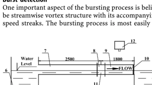
The experimental apparatus is shown in Fig. 1. The flow system is a stainless steel flume, 4.3 m long, 0.32 m wide, and 0.1 m deep. Water or surfactant solution of constant temperature was circulated in it. A fully developed flow was established in the region of 2.5 m downstream from the inlet of the flume. This was confirmed by the measurements of both the water and surfactant velocity profiles. Data for the present research were taken using a hot-film anemometer. The standard 90conical probe was connected to a tra-versing mechanism. The mechanism has a spatial resolution of 10lm. The anemometer signal was transmitted in digital code through an acquisition system to a PC. For water and drag-reducing solution the hot-film probe was calibrated in a 0.9 m diameter stainless steel tank using a specially designed rotating device. In this case the probe was connected to a rod driven by an AC motor controlled by a frequency and voltage vector control system. The frequency range of the motor was 0–120 Hz, adjustable in increments of 0.01 Hz. For water flow the probe was also calibrated in a water flume. For both calibration methods the results are in agreement. The calibration was rechecked periodically. When the sensor had drifted from the previous calibration by more than 2% the data were rejected and the calibration process was repeated. We determine that the uncertainty in a single measurement of the streamwise velocity is 3%. Turbulence measurements in drag-reducing solution were not carried out. Their absolute accuracy is poorer than in the solvent, because the heat transfer law used to calibrate the anemometer does not hold in drag-reducing solutions.

2.2

Burst detection

One important aspect of the bursting process is believed to be streamwise vortex structure with its accompanying low-speed streaks. The bursting process is most easily

characterized by a sharp acceleration of the wall-normal velocity. This feature of the bursting process was used as a detection technique. It was generally accepted that the coherent structures form in the region 5<y+<30 from the wall.

The structures were detected by placing a 35lm diameter wire in the spanwise direction at a heighty+=15, and heating the wire electrically. This diameter, with the local velocity, yieldsRe=3, which is well below the critical value of vortex shedding. The length of the wire was 0.27 m and it was located 2.5 m from the entrance to the flume. The existence of slightly heated vortices that were lifted from the bottom of the flume was verified by visu-alization of the temperature field on the free surface of the flume flow. The scheme is shown in Fig. 2.

The infrared radiometer (IR) was used to detect the thermal spots as they arrived at the water surface. It was located 1.2 m above the water surface and was able to detect temperature changes on the water surface for a distanceL+=2,300 in the flow direction. The coherent structures were heated by the wire, and, after bursting, they arrive at a water surface and appear on the water surface as a thermal spots. These spots were clearly visible to the IR, since their temperature was about 1C higher than the surrounding liquid. The spots were visible on the water surface for about 1 s, and then they faded away. The salient features of the thermal spots are clear enough to aid in the calculation of the number of new spots and their position in the streamwise and spanwise directions. From the video recording we counted the number of new spotsNxas they appeared on the interface in the bandz+=±50 at the center of the flume. The spot frequency isfs=Nx/tsm, wheretsmis the sampling interval. As the time between bursts in the present study was from 2 to 6 s a sampling frequency of 25 Hz was chosen, with a sampling time of 1,500 s. We also counted the number of spots,Nx,z, which appeared over whole width,z, of the interface. The spot frequency per unit of span was calculated asFs=Nx,z/(z·tsm).

3

Experimental results 3.1

Mean velocity profile and wall shear stress

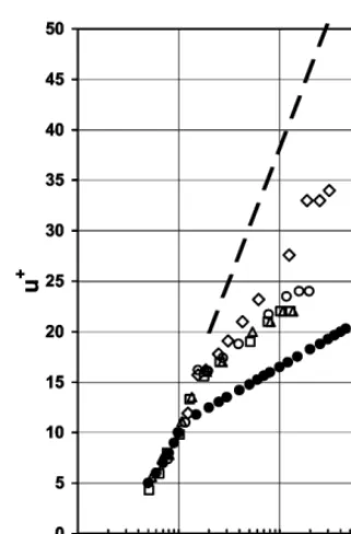
The dimensionless mean velocities,U+versusy+, are presented in Fig. 3, whereU+=U/u_{,Uis the local mean}

Fig. 1. Flow facility:1exit tank,2pump,3flow control valve,4

flowmeter,5grid,6entrance tank,7development section,8test section,9section of thermal spots visual detection,10wave

absorber,11heated wire,12IR camera Fig. 2. Schematic diagram of the visual bursting detection

velocity,u ¼pffiffiffiffiffiffiffiffis=qis the friction velocity,sis the shear stress,q is the density,yis the distance from the wall, y+=yu_{/m,mis the kinematic viscosity. As has already been}

noted in the literature, the profiles of surfactant solution are strikingly different from that obtained for water. The dashed line in Fig. 3 is Virk’s (1975) asymptote for max-imum drag reduction.

Wall shear stress for water in the flume was calculated from the average velocity profile using the equation U+=2.5ln(y+)+5. The mean velocity profile was fitted to this line by adjustingu_{so that the experimental values of}

U+ andy+agree with the ‘‘law of the wall’’. This velocity distribution and the friction velocity are in agreement within ±5% (95% confidence level) with measurements by Kaftori et al. (1994). The wall shear velocities in the drag-reducing flows in the flume were estimated by measuring velocity gradients in the viscous sublayer.

It should be pointed out that it is more appropriate for drag-reducing solutions to use a wall shear velocity, computed from the velocity gradient in the sublayer, because the ‘‘law of the wall’’ depends on the value of the shear velocity. The data of Donohue et al. (1972) and Komori et al. (1989) are also based upon the velocity gradient in the sublayer.

The wall shear velocity in DRS was determined by measurements made using the probe inside the viscous sublayer, where the average velocity varies linearly with the distance normal to the wall. The wall shear velocity was determined as:

u ¼ðmdU=dyÞ0:5 ð1Þ

The shear viscosity of surfactant solution was deter-mined with a Rheometrics Fluids Spectrometer RFS II (TA Instruments, New Castle, DE, USA)using a Couette system

in the shear rate range of 0.1–1,000 s)1 (Hetsroni et al. 2001). The standard deviation was 4%. The kinematic viscosity was determined using a Cannon-Fenske (Cannon Instrument Corp., State College, PA, USA) capillary vis-cometer at a shear rate of 5,000 s)1. The viscosity of the solution used in this research, as measured with the cap-illary viscometer, did not exceed the value for water by more than 25% (Hetsroni et al. 1997).

The wall shear stress was calculated as:

s_s¼ðuÞ2=q ð2Þ

The measured wall shear stress for the surfactant solution can be compared to the wall shear stress for the water by

% DR¼100ðs_ws_sÞ=s_w ð3Þ

where %DR is the percentage drag reduction, andswis the wall shear stress for water flow.

3.2

Bursting frequency 3.2.1

Visual observations

Figure 4 shows a typical example of a picture reproduced from the video motion frames. The picture is a plan view, where the water moved from the left to the right. The field

Fig. 3. Mean velocity profiles. 530 ppm Habon G flow:triangle

Re=3,700,square Re=4,200,circle Re=6,200,diamond Re=10,000;

solid circlewater flow

Fig. 4. Thermal spots on the water surface:asingle burst event,

bthermal spots from two ejections

of view shown in Fig. 4 is about 5 cm in the spanwise direction and 8.5 cm in the streamwise direction. The initial diameter of the new spot shown in Fig. 4a is about 0.01 m. During their displacement the spots grow, the evolution of the motion can be visually observed and demonstrated only by a time sequence of frames. It should be noted that new spots are visibly much clearer in the pictures. Many of them appear as single structures, but a pair of spots can also exist, as is shown in Fig. 4b. Corino and Brodkey (1969) also observed groups of multiple ejections and noted that on numerous occasions the ejection first appeared at a particular position within the field, and while it was in progress other ejections occurred at adjacent downstream positions. In Fig. 4b there appear two simultaneous ejections in the field of view. This figure corresponds closely to the observations of Corino and Brodkey (1969), where two ejections occur. Groups of multiple ejections were also observed in the flow visuali-zation results obtained in the study of Bogard and Tiederman (1986). They showed that an occurrence of a group of closely spaced ejections can be directly associated with break-up of a single streak. Tardu (1995) showed that solitary events clearly separated in time from each other have been categorized as single ejection bursts. Cluster events have been categorized as multiple ejection bursts. Tardu (2002) suggested that the multiple ejection burst is the manifestation of a package containing large and small time scales. In our study the multiple spots were counted as one burst.

The information of bursting frequency was obtained by using the technique of scalar transport on the water sur-face. To directly clarify both the generation process of surface-renewal motions and the scalar transfer mecha-nism we need a sophisticated image-processing technique, which can simultaneously measure instantaneous velocity and temperature (concentration) in the whole flow field. However, even if the latest image-processing technique is applied it is still impossible to get an image-processing instrument that is powerful enough.

However, direct numerical simulations (DNS) may clarify numerically the relationship between the turbulence structure and scalar transport mechanism across a zero-shear gas–liquid interface. The DNS of the time-dependent three-dimensional Navier–Stokes and scalar transport equations were produced by Komori at al. (1993) for an open-channel flow with a zero-shear gas–liquid interface. It was shown that eddies generated by the bursting motions in the wall region are lifted up toward the free surface, and they become the surface-renewal eddies. This means that the scalar transfer across the gas–liquid interface is promoted by bursting. Identifying bursts by this method was also evaluated experimentally by previous investigators and in the present study. The relationship between surface-renewal motions and bursting in the near wall region has been investigated experimentally by Komori et al. (1989) through mass-transport experiments. A point source was located aty+=15 in an open-channel flow and the concentration spots that arrived at the free surface were counted. Komori et al. (1989) showed that surface-renewal motions originate in the bursting phe-nomena in the buffer layer, and that almost all the upward ejecting eddies became surface-renewal eddies. The mass transfer across the gas–liquid interface is generally con-trolled by the turbulence structure in the buffer zone. In the present study the bursting phenomena was connected with thermal spots on the water surface, created by heated coherent structures aty+=15. It should be stressed that the method based on a visual study of bursting by the IR technique did not involve a subjective treatment of time-averaged signals in the viscous layer. We counted the number of thermal spots on the fluid surface.

The question is how many of the bursts reach the interface? Komori et al. (1989) showed that the relation between the surface-renewal frequency,fs+, and bursting frequency,f+=fm/u2_{, is extremely high and is given by} fsp+=0.9f+, wherefs+andf+are scaled with the variables u_{andm. The results of the dimensionless frequency of the}

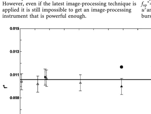
bursts,f+, in the water flow are shown in Fig. 5 as a

Fig. 5. Water flow. Dimensional bursting

fre-quency vs. Reynolds number.Triangle

2h=0.037 m,square2h=0.050 m,solid square

2h=0.085 m,solid triangle2h=0.093 m;solid circleKomori et al. (1993)

function of the Reynolds number,Re=2hUm/m, where 2 h is the flow depth, andUm is the mean bulk velocity. The results presented in Fig. 5 were obtained under conditions in which the flow depth ranged from 0.037 to 0.093m, and are in agreement within the experimental uncertainty. The average bursting frequency in water flow can be estimated asf+=0.0107. The measurements of the bursting frequency by Kline at al. (1967) and by Komori et al. (1989) give an average bursting frequency off+=0.0100 andf+=0.0120, respectively. The results of the present study agree with previous investigations. We did not observe any thermal spot at the free surface in experiments with flow of sur-factant.

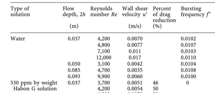
Figure 6 shows the bursting rates per meter,F versus wall shear velocity. In this figure the data of Donohue et al. (1972) and the data of Achia and Thompson (1977) are also shown for both water and drag-reducing solutions. The solid line represents the correlationF¥u3_established by Kline et al. (1967). In the clear water flow, the agree-ment between the present study and the predictions of Kline et al. (1967) is quite good. The drag-reducing data of Donohue et al. (1972), and Achia and Thompson (1977) show significantly reduced spatially averaged bursting rates. It is seen that the dependence F¥u3_{does not} describe the relation between the bursting rates and wall shear velocity in drag-reducing flows. The main experi-mental results are given in Table 1.

In Fig. 6, the drag-reducing data show significantly reduced averaged bursting rates. The amount and

character of this reduction can best be illustrated by a numerical example. When the water flow and flow of 50 ppm by weight Separan AP30 (Dow Chemical Co.) solution used by Achia and Thompson (1977) are com-pared at the same shear velocityu=0.0345 m/s, it is seen thatF=1,800 bursts/ms for the drag-reducing flow is considerably lower thanF=5,000 bursts/ms for water. From the intersection of the line CD described in the data of Donohue et al. (1972) with the line ofu=0.0345 m/s one can conclude that the bursting rate is about F=200 bursts/ms. Thus, a decrease inuonleads to a significant decrease inF.

The onset shear velocity of drag reduction may be determined from Fig. 6. For the 50 ppm Separan AP30 solution the onset shear velocity of drag reduction,

uon=0.017 m/s was found by Achia and Thompson (1977)

as the intersection of the lineFu1.25_{for drag-reducing} solution with the lineFu3_{for water. Using this method} the value of the onset shear velocity of drag reduction for solutions used by Donohue et al. (1972) may be deter-mined to aboutuon=0.006 m/s. This value agrees with that determined from streak spacing measurements by Hetsroni et al. (2003). Further reference to the onset of drag reduction will be made in the discussion.

4

Discussion 4.1

Bursting and streak spacing

Previous experiments have shown an increased spacing of sublayer streaks for drag-reducing flow while the bursting rate has decreased. This increased spacing led Donohue et al. (1972) to hypothesize that the ability of the drag-reducing solution to resist vortex stretching could inhibit the formation of wall-layer streaks. The modern, widely accepted explanation of ‘‘bursting’’ is the advection of spatially distributed streamwise vortices and related structural features in the flow direction accompanied by the rapid temporal growth. Already a consensus has been reached regarding the most likely reason for drag reduc-tion, based on the extensional viscosity of surfactants (Dimitropoulos et al. 1998). Macromolecules, by enhanc-ing the resistance of the fluid to extensional deformations, make the wall eddies wider and less frequent and in con-sequence less efficient in supplying the logarithmic layer with energy. The instantaneous velocity along the flow direction produces wider thermal streaks and one observes less frequent wall-layer bursts than that in Newtonian flows.

4.2

Bursting rate and the onset of drag reduction

The drag-reducing effect starts when the wall shear stres-ses is larger than some threshold value, which depends on the concentration and the kind of additives. The first step of the hypothesis presented here is an attempt to relate the bursting rate in drag-reducing flow,F, to the onset of turbulent drag reduction. This hypothesis states that: the onset of drag reduction in turbulent flow occurs when a line that describes the dependenceF=f(u_{) for}

Fig. 6. Spatial averaged bursting rates in water and drag-reducing

flows. Water—present study:triangle2h=0.037 m,square

2h=0.050 m,solid square2h=0.085,solid triangle2h=0.093 m;

plusKline et al. (1967);circleDonohue et al. (1972);diamond

Achia and Thompson (1977). Drag-reducing solutions—solid circleDonohue et al. (1972), 139 ppm by weightsolution of polyethylene oxide;solid diamondAchia and Thompson (1977), 50 ppm by weight solution of Separan AP30

drag-reducing solution crosses the lineFu3_that describes dependence for Newtonian fluids.

The data in Fig. 6 represent spatially averaged bursting rates in water and drag-reducing flows. Points at which the linesF=f(u) cross the lineFu3 _{indicate a threshold} value (onset of wall shear velocity,uon, for particular drag-reducing solution). The drag reduction takes place at values ofuhigher than the onset wall shear. The onset of shear velocity,uon, is not a universal constant. It should be dependent on the solvent and on the concentration of the drag-reducing solution.

It is apparent from Fig. 6 that the value of uonfor drag-reducing solution used in the study of Donohue et al. (1972) is considerably lower than that for the solution used by Achia and Thompson (1977). Figure 6 shows that in this case the bursting rate for the solution used in the study of Donohue et al. (1972) is also lower than that for the solution used by Achia and Thompson (1977). The 530 ppm by weight of Habon G (Hoechst, Frankfurt-am-Main, Germany) solution has significantly lower value of the onset velocity (uon<0.002 m/s) compared to the 139 ppm polyethylene oxide-FRA solution (uon about 0.006 m/s) used by Donohue et al. (1972) and 50 ppm Separan AP 30 solution (u

onabout 0.017 m/s) used by Achia and Thompson (1977). The experimental results of the present study permit one to conclude that in Habon G flow drag reduction occurs at the extremely low value of the onset velocity. In this case the flow is turbulent, and the velocity profile is not parabolic. However, the obser-vation of zero bursting rate implies that turbulence is not produced by the classical method.

5

Conclusion

An experimental technique was developed, which permit-ted detailed observations of burst distribution in spanwise and streamwise directions. Infrared thermography was used to detect and measure the frequency of the coherent structures as they arrive at the interface of a flume. These structures are formed near the bottom of the flume, and then they lift toward the interface, where they are detected as thermal spots.

From experiments in water flow, the frequency of bursts per unit of span, and also an average frequency at a point was determined. It is important to note that we have

good agreement between data reported in the literature and visual results obtained in the present study. There is also an additional physical insight, which can be learned from the spot emergence on the water surface. The sur-face-renewal motions originate in the bursting motions, which occur in the buffer region. That is, the fluid, which is strongly lifted towards the outer layer by the bursts, almost always arrives at the free surface and renews it. Heat and mass transfer across the gas–liquid interface is dominated by the large-scale eddies, and depends on the surface-renewal frequency.

Experiments performed in high drag-reducing 530 ppm Habon G solution revealed that bursting was not observed. The experimental results of the present study permit one to conclude that in Habon G flow drag reduction occurs at an extremely low value of the onset velocity. In this case the flow is turbulent, the velocity profile is not parabolic, and the observation of zero bursting rate implies that turbulence is not produced by the classical method. It should be mentioned that the onset of drag reduction depends on the relaxation time, which represents a drag-reducing solution’s elastic property. Additional studies are required to clarify the properties of surfactant solutions and the length scale associated with bursting in drag-reducing flow.

References

Achia BU, Thompson DW (1977) Structure of the turbulent boundary in drag-reducing flow. Fluid Mech 81:439–464

Adrian RJ, Meinhart CD, Tomkins CD (2000) Vortex organization in the outer region of turbulent boundary layer. J Fluid Mech 422:1–53

Bogard DG, Tiederman WG (1986) Burst detection with single point velocity measurements. J Fluid Mech 162:389–413

Chara Z, Zakin JL, Severa M, Myska J (1993) Turbulence measure-ments of drag reducing surfactant systems. Exp. fluids 16:36–41 Corino ER, Brodkey SR (1969) A visual investigation of the wall

region in turbulent flow. J Fluid Mech 37:1–30

Dimitropoulos CD, Sureshkumar R, Beris A (1998) Direct numerical simulation of viscoelastic turbulent channel flow exhibiting drag reduction: effect of variation of rheological parameters. J Non-Newtonian Fluid Mech. 79:433–468

Donohue GL, Tiederman WG, Reischman MM (1972) Flow visuali-zation of the near-wall region in drag-reducing flow. Fluid Mech 56:559-575

Hetsroni G, Zakin JL, Mosyak A (1997) Low speed streaks in drag reduced turbulent flow. Phys Fluids 9:2397–2404

Table 1. Experimental results

Type of solution

Flow depth, 2h

Reynolds numberRe

Wall shear

velocityu Percent_{of drag}

reduction

Bursting frequencyf+

Bursting rate per meter,F

(m) (m/s) (%) (burst/ms)

Water 0.037 4,200 0.0070 0.0102 30 4,800 0.0077 0.0107 46 7,100 0.011 0.0103 130 12,000 0.017 0.0110 550 0.050 3,100 0.0042 0.0104 6.7 0.085 4,700 0.0035 0.0108 4.0 0.093 9,900 0.0060 0.0100 19 530 ppm by weight

Habon G solution 0.037 3,7004,200 0.00510.0054 4650 0 0 6,200 0.0078 50

10,000 0.012 53

Hetsroni G, Zakin JL, Lin Z, Mosyak A, Pancallo EA, Rozenblit R (2001) The effect of surfactants on bubble growth, wall thermal patterns and heat transfer in pool boiling. Int J Heat Mass Transfer 44:485–497

Hetsroni G, Mosyak A, Talmon Y, Bernheim-Groswasser A, Zakin JL (2003) The effect of cationic surfactant on turbulent flow patterns. J Heat Transfer 125:947–950

Jeong J, Hussain F (1995) On the identification of vortex. J Fluid Mech 285:69–94

Kafttori D, Hetsroni G, Banerjee S (1994) Funnel-shaped vorticle structures in wall turbulence. Phys Fluids 6:3035–3050

Kawaguchi Y, Tawaraya Y, Yabe A, Hishida K, Maeda M (1996) Active control of turbulent drag reduction in surfactant solutions for wall heating. In: Proceedings of the Symposium on Turbulent modi-cation and drag reduction, July 1996. ASME FED 237, vol 2, pp 47–52

Kline SJ, Reynolds WC, Schraub WC, Runstadler FA (1967) The structure of turbulent boundary layers. Fluid Mech 30:741–773 Komori S, Murakami Y, Ueda H (1989) The relationship between

surface renewal and bursting motions in an open-channel flow. Fluid Mech 203:103–123

Komori S, Nagaosa R, Murakami V, Chiba S, Ishii K, Kuwahara K (1993) Direct numerical simulation of three-dimensional open channel flow with zero-shear gas–liquid interface. Phys Fluids A5:115–125

Luchik TS, Tiederman WG (1988) Turbulent structure in low-con-centration drag-reducing channel flows. Fluid Mech 190:241–263 Podvin B, Gibson J, Berkooz G, Lamley J (1997) Lagrangian and

Eulerian view of the bursting period. Phys Fluids 9:433 Robinson SK (1991) Coherent motions in the turbulent boundary

layer. Ann Rev Fluid Mech 23:601–639

Tardu S (2001) Active control of near wall turbulence by local un-steady blowing J Fluid Mach 439:217–253

Tardu SF (1995) Characteristics of a single and clusters of bursting events in the inner layer. 1. VITA events. Exp Fluids 20:112–124 Tardu SF (2002) Characteristics of a single and multiple bursting

events in the inner layer. Part 2. Level-crossing events. Exp Fluids 33:640–652

Tiederman WG, Luchik TS, Bogard DG (1985) Wall-layer structure and drag reduction. Fluid Mech 156:419–437

Virk PS (1975) Drag reduction fundamentals. AIChE J 21:625–656 Warholic MD, Massah H, Hanratty TJ (1999a) Influence of

drag-reducing polymers on turbulence: effects of Reynolds number, concentration and mixing. Exp Fluids 27:461–472

Warholic MD, Schmidt GM, Hanratty TJ (1999b) The influence of drag reducing surfactants on a turbulent velocity field. Fluid Mech 388:1–20