Recursive grid methods to compute value sets and Horowitz–Sidi bounds

Published online 10 August 2006 in Wiley InterScience (www.interscience.wiley.com). DOI: 10.1002/rnc.1083

Recursive grid methods to compute value sets and

Horowitz–Sidi bounds

Per-Olof Gutman

*

, Mattias Nordin

and Bnayahu Cohen

1

Faculty of Civil and Environmental Engineering, Technion – Israel Institute of Technology, Haifa 32000, Israel 2_{Volvo Construction Equipment Components, 63185 Eskilstuna, Sweden}

3_{M.E.S., Medical Electronic Systems Ltd., P.O.B. 3017, Ceasarea 38900, Israel}

SUMMARY

In this paper, recursive extensions to the standard equidistant grid method are proposed whereby the gridding is adapted locally such that a prescribed distance is achieved between neighbouring points in the computed value set (template). Also presented is the Prune algorithm, which finds the outer border of a value set defined by a set of points whose nearest neighbour lies within a prescribed distance. The Prune algorithm is part of the recursive grid methods, but can also be used independently with other methods to compute value sets. As an alternative to analytical or search algorithms, a recursive grid algorithm is presented to compute Horowitz–Sidi bounds (QFT bounds, or boundaries). Isaac Horowitz’s contribution

to computational methods for QFT is outlined in the perspective of the presented algorithms. Copyright#

2006 John Wiley & Sons, Ltd.

Received 29 October 2005; Revised 11 May 2006; Accepted 11 May 2006

KEY WORDS: quantitative feedback theory (QFT); robust control; template generation; bound generation

1. INTRODUCTION

By 1984 Isaac Horowitz was an active and well-established professor at the Department of Mathematics of the Weizmann Institute of Science. QFT was already well developed by Horowitz and his numerous graduate students, from the first QFT paper [1] to the recent

*Correspondence to: Per-Olof Gutman, Faculty of Civil and Environmental Engineering, Technion – Israel Institute of Technology, Haifa 32000, Israel.

y

E-mail: [email protected] z

E-mail: [email protected] }_{E-mail: [email protected]}

Contract/grant sponsor: NUTEK; contract/grant number: 9156700 Contract/grant sponsor: Israel Institute of Technology

PhD thesis by Yaniv, published as a paper [2]. All Horowitz’s students applied the new methods to various examples, and wrote appropriate software. The mathematician Dr Linda Neumann was employed by Horowitz as a scientific programmer, a QFT design program had been written in FORTRAN, and many extremely challenging design problems were solved, e.g. the 55 MIMO flight control problem [3].

Professor Horowitz was very interested in the computerized implementation of QFT design and analysis tools. In his original design program value sets (templates) of parametric rational functions, with each parameter belonging to an interval, were computed, for each chosen frequency, by thegrid method, whereby each parameter interval is equidistantly gridded, and the values of the rational function are computed at the grid points in the parameter space. The grid method is also the only template computation method in the Horowitz inspired Reference [4], which was also written in FORTRAN and made use of the user interaction modules of the control design and analysis programs SYNPAC, and IDPAC developed at Lund Institute of Technology, Sweden, [5], and in the QFT Toolbox for Matlab [6], and in the original software developed by the Air Force Institute of Technology, Ohio [7–9].

It is however well known, see, e.g. Reference [10], that the grid method may fail to yield a set of template points suitable for control systems design. Therefore, many alternative template computation methods have been proposed over the years such as: (1) the Qsyn}the Toolbox for Robust Control Systems Design for use with Matlab [11] in which the more efficient template computation algorithms were developed; (2) the Real Factored Form method [10]; (3) the Recursive Edge Grid Method [12]; and (4) the Recursive Grid Methods together with a ‘pruning’ algorithm to find the outer border of a template, as illustrated in this paper [13].

It should be noted that a Horowitz–Sidi bound for a given specification and for a given frequency,o;[1], is the border in the complex plane between the feasible and infeasible sets of the nominal compensated open loop frequency function valueLnomðjoÞ ¼GðjoÞPnomðjoÞwhere

Gdenotes the compensator, andPnom the nominal plant case.LnomðjoÞbelongs to the feasible set is the specification satisfied for all plant cases at the given frequency o:

In Horowitz’s original software, see also the Matlab m-files on page 466 in Reference [14], a Horowitz–Sidi bound for a given frequencyoand a given specification is computed point-by-point as a line search along constant phase grid lines in the Nichols chart, conceptually as follows.

Algorithm 1

1. Choose a phasef;

2. Choose an initial very high gain,A;

3. Choose implicitly an appropriate GðjoÞsuch thatjLnomðjoÞj ¼A;and argðLnomðjoÞÞ ¼f; 4. Check if the specification is satisfied. If No, let A¼AþdA; if Yes, let A¼ADA:

Return to point 3, until the upper Horowitz–Sidi bound point is found with required accuracy, or the desired gain range is searched;

5. If the upper Horowitz–Sidi bound point was found, choose an initial very low gain,a; 6. Choose implicitly an appropriate GðjoÞsuch thatjLnomðjoÞj ¼A;and argðLnomðjoÞÞ ¼f; 7. Check if the specification is satisfied. If No, let A¼AdA; if Yes, let A¼AþDA:

Return to point 5, until the lower Horowitz–Sidi bound point is found with required accuracy (note that the upper and lower bound points may co-incide);

Graphically, Algorithm 1 is very elegant. It is performed by sliding a given template with its nominal along constant phase grid lines in the Nichols chart, while investigating if the given specification is satisfied. The bound points are marked on the Nichols chart. Clearly, Isaac Horowitz used his deep control theoretical understanding when proposing this algorithm.

Algorithm 1 was used in Reference [4] and is the main algorithm in Reference [6]. However, Algorithm 1 does not compute the correct Horowitz–Sidi bound, if the bound intersects a given phase grid line more than twice, since the complete phase grid line is not investigated. See Figure 7. Bailey et al.[15] were the first to investigate this phenomenon ofmulti-valuedbounds.

In general, some search procedure is necessary to find the Horowitz–Sidi bounds. In certain cases, notably for sensitivity specifications, the Horowitz–Sidi bounds can be computed explicitly by quadratic inequalities, [16], which represents a clear improvement over Horowitz’s original, and is also used in Reference [6]. Here, the recursive grid method for the computation of Horowitz–Sidi bounds used in Qsyn since its inception [11] is presented, noting that it was independently discovered also in Reference [17]. Other contributions to the bound computation problem are, e.g. References [18–21].

We recognize with gratitude the contribution by Isaac Horowitz who together with his students developed the very practical and useful control design technique called QFT. His inspiration guided us and others to create efficient computational tools for QFT.

This paper is organized as follows: The problem of computing value sets is discussed in Section 2, together with a brief literature survey. The Prune algorithm is presented in detail in Section 3, together with an illustrative example. The recursive grid algorithms are outlined in Sections 4 and 5, together with a physical example. The recursive bound computation algorithm is found in Section 6. A brief conclusion and an acknowledgement concludes the paper.

2. COMPUTING VALUE SETS

Example

Consider the real-valued scalar function fðxÞ ¼1=ð0:0001þ ðx0:95552928514718Þ2Þ; of the real-valued variablex2 ½0;1:It is easy to analytically calculate that the value set (range) off is

½1:09512686477738;10 000:It is however not trivial to find the upper boundary of the range by numerical methods. If you would use the Grid Method and divide the x-interval equidistantly into, e.g. 1001 points, then you will get fð0:955Þ ¼9972:063984025603; and fð0:956Þ ¼

9977:891738555019 wherebyfð0:956Þ fð0:955Þ520;but the found maximum value is removed more than 20 units from the true upper limit 10 000. What would induce you to subdivide the

x-interval further? How do you know that enough is enough? For comparison, the Matlab functionfplot(‘1/(0.0001+(x-0.95552928514718)^2)’,[0,1],1e-3)gives the maximum as 9977.89173855495, in spite of the fact that adaptive gridding of the x-values is used, and a relative tolerance of 0.1%, i.e. 10 units, was demanded.

The most straightforward, but computationally intensive method is the Grid method, whereby each parameter interval is equidistantly gridded, and the values of the rational function are computed at the grid points in the parameter space. When the Edge Theorem holds, [23], it is sufficient to grid the edge in the parameter space, i.e. in turn, each parameter is gridded while all the others are kept at an interval end points. The edge grid method has been extended to the recursive edge grid method in Reference [12] where each edge is gridded adaptively by, e.g. bisection, to achieve a prescribed resolution of the value set, i.e. a prescribed maximum distance between the computed neighbouring points. The recursive edge grid method compares favourably with the method of Reference [23] from a computational point of view.

For the purpose of investigating robust stability, [24], or for robust control system design, [1], only the outer border of the value set is needed. Most of the above-mentioned methods give interior points as well. This paper presents an algorithm that finds the outer border points, under the assumption that the value set was computed with a known resolution. Appropriately, this algorithm is called the Prune algorithm. The algorithm may substantially reduce the computational effort when computing value sets for tree-structured transfer functions, [24]. An algorithm akin to the Prune algorithm in Reference [13] was published several years later in [30]. One aim of this paper is the presentation of recursive grid algorithms that give a prescribed resolution of the outer border of the value set, for all types of parametric frequency functions for which the original equidistant grid method is applicable. It should be noted that also un-structured uncertainty of the type PðjoÞ ¼PnomðjoÞ þMðjoÞor PðjoÞ ¼PnomðjoÞð1þMðjoÞÞ;

r¼ jMðjoÞj4mðoÞ; f¼argðMðjoÞÞ 2 ½0;2p can be parameterized in rand f; see References [11, 31]. In the first recursive grid method I, the parameter space is recursively gridded such that the prescribed resolutions is achieved. The Prune algorithm is applied during and after the recursion.

It should be noted that all grid methods compute underbounds of the true value set, unless the parametric rational function has some special structure [23, 10], or satisfies some regularity condition [32]. This restriction holds, by the way, also for function plotting routines in programs like Matlab [33]. The second recursive grid method is applicable when a Lipschitz constant is known for the parametric rational function. Then interior points sufficiently far away from the hitherto computed interim outer border of the value set need not to be computed at all, resulting in substantial computational savings. Recursive gridding is interleaved with pruning.

A breakthrough in template computation was achieved in Reference [34] and papers referenced therein, where the outer bounds of value sets of parametric frequency functions are computed without knowing a Lipschitz constant, by the use of interval analysis. The transfer function is decomposed into elementary functions, and the parameter intervals subdivided, such that the gain and phase extent can be analytically computed on the subintervals. The proposed method is shown by example to be computationally superior to other methods, including the ones in this paper.

3. THE PRUNE ALGORITHM

Without restriction, consider a discrete set of disjoint complex pointsV¼ fv1;v2;. . .;vng;where identical points are considered as one. Introduce

Definition 1

A setVis said to bee-connected if for every pair of pointsvi;vj2V;there is a sequence of points

Vij¼ fv1ij;vij2;. . .;vkijg V such thatv1ij¼vi;vkij¼vj andjvmij v mþ1

Let nowV bee-connected and construct

CðVÞ ¼[

n

i¼1

x: jxvij4

e

2

n o

ð1Þ

It follows from (1) and Definition 1 that CðVÞ is a connected, but not necessarily simply connected set in the complex plane. Let@CðVÞdenote the outer border ofCðVÞ;i.e. the border encountered when approachingCðVÞfrom infinity. A pointv2Vis called aninteriorpoint ofV

if@CðVÞ ¼@CðV fvgÞ:A pointv2V is called aborderpoint ofVif it is not aninteriorpoint. LetBðVÞ Vbe the set ofborderpoints ofVandIðVÞ ¼V BðVÞthe set ofinteriorpoints of

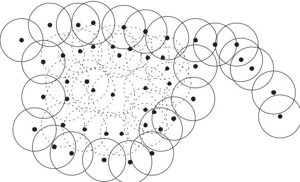
V:It is easily shown thatBðVÞis alsoe-connected and that@CðBÞ ¼@CðVÞ:Define thee-circles

ci¼ fz: jzvij ¼e=2g;i¼1;2;. . .;n:In Figure 1 an example ofVwith itse-circles are plotted.

BðVÞis the set of all points with solid circles andIðVÞis the set of points with dotted circles. It is obvious from the construction ofCðVÞthat@CðVÞis a continuous curve of circular arcs

AðVÞ ¼ fa1;a2;. . .;akg: Each of these arcs is associated to some border point in a sequence

Bn

ðVÞ ¼ fb1;b2;. . .;bkg:It holds that

BðVÞ ¼[

k

i¼1

fbig ð2Þ

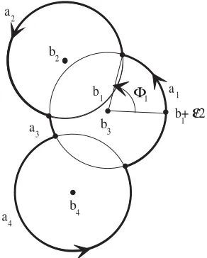
Note that the arcs are unique but two or more arcs can have the same centre, and therefore not all points in Sk_i¼1fbigneed to be disjoint, see Figure 2.

We can now construct an algorithm, the Prune algorithm, which finds BðVÞby recursively finding the points ofBn

ðVÞ:This can be done by finding these circular arcs and their associated centres inV:The idea is to track@CðVÞand recursively find the consecutive arcs inAðVÞ:The algorithm consists of three parts: (i) Find a starting pointb1 and its successorb2:(ii) Given to

pointsbi andbi1 find the successorbiþ1:(iii) A terminating condition to know whenCðVÞis encircled. Let us now proceed with the three steps:

(i) A starting pointb1 can be found by

b1¼arg max

v2V realðvÞ ð3Þ

i.e. one of the rightmost points inV:It is clear that the pointb1þe=2 must belong to@CðVÞ:It is also clear that, remembering that the points in V are disjoint, no other point v2V gives a contribution to@CðVÞatb1þe=2:Henceb1is aborderpoint andb1þe=22a1;see the example in Figure 2. Then follow the arc a1 in the positive direction until the first time it intersects another e-circle round some point v2V: All possible candidates v2V for intersection must satisfy 05jvb1j4e:SinceV ise-connected there must be at least one suchv:Define the angle

f₁ðvÞ ¼/_{ðvb1Þ arccosðjb1vj=eÞ ð4Þ}

The first circle that intersectsa1is the one with the smallest anglef1ðvÞ;seef1ðb2Þin Figure 2. It now follows that

b2¼arg min 05jvb1j4e

f₁ðvÞ ð5Þ

If the minimizing argument in (5) is not unique, there are several circles that intersect in the same point ofa1:In that case choose the minimizingvof (5) farthest away fromb1;because the others only give a contribution to @CðVÞat the intersection point.

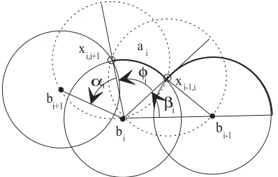
(ii) Consider two consecutive points bi1;bi2BnðVÞ; see Figure 3. The intersection point betweenai1andaiis denotedxi1;i:The next pointbiþ12BnðVÞis found by following the arcai from the intersection point xi1;i until another intersection is encountered. All possible candidates v2V for intersection must satisfy 05jbivj4e:Since V ise-connected there are always possible candidates. Note that bi1¼biþ1 is possible. The pointbiþ1can now be found

a b

b

1 2

3

b+ /2₁

b₄ b₁ a₂

a₃

a₄

1

Figure 2. A three point example of how the Prune algorithm works. Note thatBn

ðVÞincludes four points

by choosing the candidate with the smallest anglef_iðvÞ;see Figure 3. Geometry gives

aiðvÞ ¼arccosðjbivj=eÞ ð6Þ

bi¼arccosðjbi1bij=eÞ ð7Þ

aiðvÞ þbiþfiðvÞ ¼/

vbi

bi1bi

ð8Þ

from which

f_iðvÞ ¼/ vbi

bi1bi

arccosðjvbij=eÞ arccosðjbi1bij=eÞ ð9Þ

biþ1 is now given by

biþ1¼arg min

05jvbij41fiðvÞ ð10Þ

If the minimizing argument in (10) is not unique choose the point farthest away frombi;because the other minimizing arguments only gives a contribution to @CðVÞ at the point xi;iþ1;which already is given by ai:

(iii) Note that since (10) only depends on the two previous points inBn

ðVÞwe reach a closed orbit inBn

ðVÞas soon asb1¼bkþ1andb2¼bkþ2;because it follows then from induction that

bm¼bkþmfor all integersm>0:We have then reached the starting arca1and can terminate the recursion. Now the sequence Bn

¼ fb1;b2;. . .;bkg V with the required conditions is found. In other words we have encircled the setVand found theborderpoints. Consider Figure 3. An interpretation of one step in the algorithm works is that it takes the dotted circle of radiuse=2 touchingbi1 andbiand rolls it aroundbiuntil it touchesbiþ1:Hence all the consecutive points inBn

ðVÞis given by rolling a circle with diameterearound the points ofV:The algorithm will catch concavity with a curvature less than 2=e; which is evident from the rolling circle interpretation of the Prune algorithm.

b b

b x

x

i-1 i

i+1

i-1,i i,i+1

i

i i

a_i

-15 -10 -5 0 5 10 15 20 25 -15

-10 -5 0 5 10 15 20

-15 -10 -5 0 5 10 15 20 25 -15

-10 -5 0 5 10 15 20

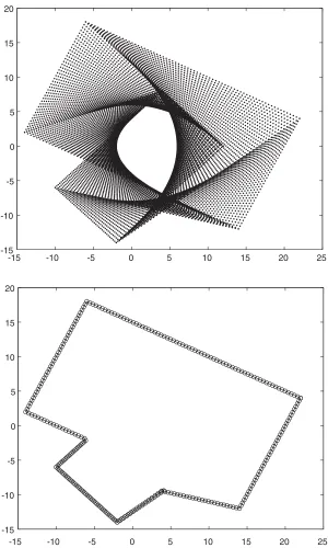
Figure 4. The value setV(upper plot) with 13 200 points and the pruned setBn

ðVÞ(lower plot) with 286 points, including thee-circles ofBn

3.1. Example

Let us consider an example taken from [24, pp. 158–159], with two value setsA¼ fxþi2:x2 ½2;4g and B¼ fxþiy:x2 ½3;4;y2 ½1;3g are given. We are interested in finding the border @C of the productAB:In Reference [24] it is shown that @C@A@B: In order to calculate @C the sets @A and @B are gridded with steplength 0.1 and then multiplied into a discrete set V: Note now that V is e-connected with e¼0:1 minðmaxjAj;maxjBjÞ ¼

0:2pffiffiffi550:5:We then compute an approximation of@Cby applying the Prune algorithm toV

with e¼0:5: In Figure 4 V@A@B and the approximation of @C is shown. Our implementation of the Prune algorithm in MATLAB 6.5 [33] uses the efficient sparse matrix function to find the possible candidates, i.e. points within the distance e: This example with 13 200 points is pruned in 0.56 seconds on a 1.86 GHz Pentium M computer, with a straightforward m-file implementation.

4. THE RECURSIVE GRID ALGORITHM I

Consider a continuous transfer functionPðjo;qÞ;withqan uncertain parameter vector such that

q2Q¼ fqj

%

qi4qi4q%i 8i¼1;2;. . .;lg ð11Þ

We want to compute an accurate approximation of the value set VðP;Q;oÞ ¼ fPðjo;qÞ jq2Qg; for a fixed frequency o: As pointed out in, e.g. Reference [24], dense gridding of the uncertain domain is often the only possibility to achieve this goal. But what is a ‘dense gridding’? It is obvious that this depends on the properties ofPðjo;qÞand the required accuracy. A common ‘brute force’ method is to grid the parameters equidistantly and then plot the values of Pðjo;qÞ for all these parameter combinations. Let us define a grid in the uncertainty set Qas follows: Let q*i¼ fq*1i;. . .;q*

ni

i g be a vector such thatq*1i ¼qi; q*nii ¼qi; and q*j_iq*j1_i ¼ ðqiqiÞ=ðni1Þ: With qmin¼ ½

% q1;

% q2;. . .;

%

ql; qmax¼ ½q%1;q%2;. . .;q%l and

n¼ ½n1;n2;. . .;nlwe now have the set of grid points

Qgðqmin;qmax;nÞ ¼q*1q*2 q*lQ ð12Þ

The size ofQgisN¼Qli¼1niand even for reasonably smalllthis might be prohibitively large, if a high accuracy is required. Therefore, we construct a recursive algorithm that is adaptive in the sense that it makes necessary parts of the grid progressively finer, such that ane-connected set of evaluations of the uncertain transfer function Pðjo;qÞis achieved. The steps of the Recursive Grid I algorithm are:

1. Select an initial gridQ0_g:TheQ0_g-gridding dividesQintoQl_i¼1ðni1Þsmaller uncertainty sets, so-calledQ-boxes [24]. Evaluate the transfer function at theN0gridpoints, and hence eachQ-box has got the transfer function evaluated at all its 2l vertices.

2. Select aQ-box. For each parameter,qi;check the difference between the values ofPðjo;qÞ at the end points of the edges in the direction ofqi:If one of the differences is greater thane; the grid is made finer in the qi-direction in this particular Q-box, not in the entire Q: Evaluate the transfer function at the vertices of the new, smallerQ-boxes.

-60 -40 -20 0 20 40 60 -65

-60 -55 -50 -45

phase [degrees]

phase [degrees]

Magnitude [dB]

Nichols chart : Recursive Edge Grid (i)

-60 -40 -20 0 20 40 60

-65 -60 -55 -50 -45

Magnitude [dB]

Nichols chart : Recursive Grid (ii)

S

e-connected, and whenever the end is reached of a sufficiently large branch, the Prune algorithm is used to reduce the number of memorized value set points.

4. Repeat points 2 and 3 for all originalQ-boxes. When finished, prune a last time to get the outer border of the computed value set.

4.1. Example

Consider a simplified elastic two mass system. A motor with inertiaJm¼0:4 kg m2is driving a load with inertiaJl 2 ½5:6;8kg m2:They are coupled via a shaft with stiffnessk2 ½5880;5900 Nm=rad and damping c2 ½30;300Nm=rad=s: Introducing q¼ ½Jl;k;cT2Q; the uncertain transfer function from control torque to motor speed is given by

Pðq;sÞ ¼ Jls

2_þdsþk

JlJms3þ ðJlþJmÞds2þ ðJlþJmÞks

ð13Þ

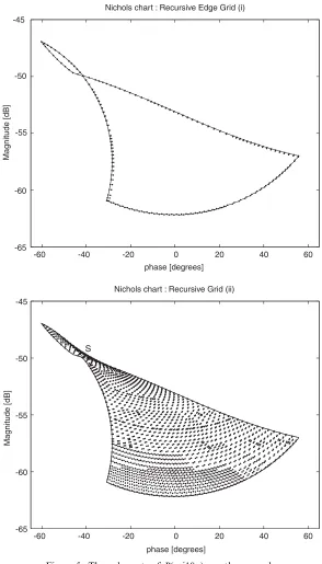
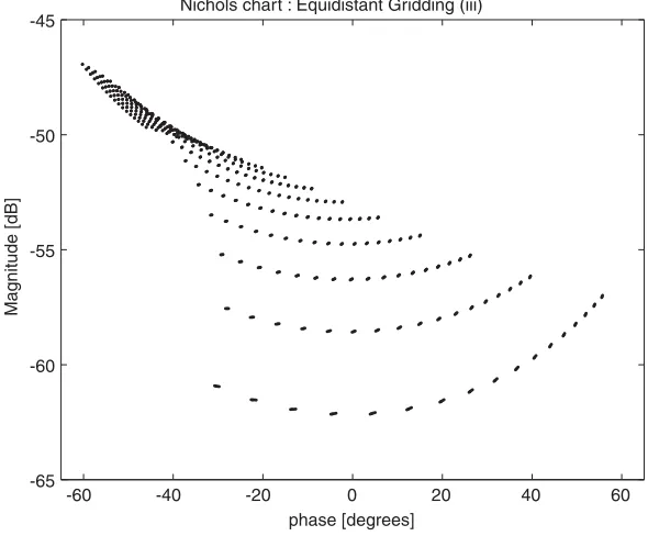
Let us compute the value set of (13) for o¼10prad=s;with three different methods: (i) The recursive edge grid algorithm [12], (ii) the recursive grid method and (iii) a ‘brute force’ equidistant gridding, see Figures 5 and 6. The required 2-norm resolution in the Nichols chart is 3:58degrees and 0:5 dB;respectively.

(i) The recursive edge grid algorithm grids every edge of Q(11) finer and finer until its transfer function values aree-connected. The total computed value set of the edges is thene-connected and suitable for pruning. In this example 302 points were computed and the pruned border had 187 points. (ii) The recursive grid algorithm I computed 4328 points and the final border size was 241 points. Note that the recursive edge grid algorithm did not give the full value set, see the area below the S in Figure 5.

-60 -40 -20 0 20 40 60 -65

-60 -55 -50 -45

phase [degrees]

Magnitude [dB]

Nichols chart : Equidistant Gridding (iii)

(iii) To compare with equidistant gridding of Q we tried a grid with 173 _{¼4913 points,} somewhat more than in (ii). Note that this computed value set is suitable for pruning only with a much larger e than required, and miss border segments with large concavity. Usually, this feature is of the grid method is even more extreme, see, e.g. the example in Reference [22].

5. THE RECURSIVE GRID II ALGORITHM

A parametric frequency functionPðjo;qÞsatisfies a Lipschitz condition, if, for a given frequency

oand for any two parameter vectorsq1;q22Q, a positive constantKðoÞis known such that

jPðjo;q1Þ Pðjo;q2Þj4KðoÞjq1q2j;wherejjdenote appropriate norms. In the initial example in Section 2 maxx2½0;1f0ðxÞ is the smallest possible Lipschitz constant. Clearly, if a Lipschitz constant is known, the required resolution of the gridding of the parameter set can be easily found as a function of the allowed error of the computed value set. In the initial example in Section 2 it is easy to analytically compute f0ðsÞ and its maximum. For parametric transfer functions it is in general non-trivial to calculate a Lipschitz constant. A numerical computation would in general entail the same order of effort as computing the value set itself.

However, the recursive algorithm in the last section can be speeded up if a Lipschitz constant for the transfer functionPðjo;qÞis known. Then, the transfer function values at pointswithina

Q-box whose vertex point values lie sufficiently far away from the hitherto computed interim outer border of the value set, also lie within that same interim border, and hence need not be computed. This means that someQ-box branches may not have to be computed to the last ‘leaf’, resulting in computational savings. The modified algorithm has to start with ane-connected set. The steps of the recursive grid II algorithm are as follows.

1. Use the recursive edge grid method [12] along the edges of the original parameter domain

Q;in order to achieve ane-connected set whose border is found with the Prune algorithm. 2. Select an initial grid Q0

g: Evaluate the transfer function at its N0 gridpoints. Define the

Q-boxes as in point 1 in Section 4.

3. Select aQ-box of which at least one of its vertex values has been included in a previous prune operation.If all its vertex values are sufficiently far away inside the interim border so that by the Lipschitz condition no interior point of the Q-box can assume a value outside the interim border,do not grid this Q-box further. Otherwise, proceed as in point 2 in Section 4. 4. Repeat the above point recursively as in point 3 in Section 4, with the difference that the prune operation is performed together with the interim border, when the number of new value points is larger than the number of interim border points. Thus, an updated interim border is computed.

5. Repeat the above until the whole ofQis covered.

6. A RECURSIVE HOROWITZ–SIDI BOUND ALGORITHM

The bound computation method presented in this section was developed in 1995 and implemented in Qsyn, see Reference [11]. Independently, the algorithm was also discovered in Reference [17] where, in addition, some computational problems around the ‘instability point’

1 are solved.

the nominal plant case. Let aspecification criterion function ZðGðjoÞ;PiðjoÞÞbe a function of the feedback controller frequency function valueGðjoÞ 2C(to be assigned),Pi;and possibly other known frequency functions, for which a specification is specified. Let zðoÞbe the specification value at frequencyo:Then a frequency domain specification may be defined as

fðGðjoÞÞ8_{ZðGðjoÞ;PiðjoÞÞ zðoÞ OP 0; 8i ð14Þ} where OP2 f¼; >;5;5;4g;andfðGðjoÞÞdenotes the left-hand side.}

Example

The common servo gain specification [1] for the standard two degrees-of-freedom feedback configuration is given by aðoÞ4jFPiG=ð1þPiGÞj4bðoÞ; 8i; with F denoting the prefilter,

b>a>0;and the frequency argument of the frequency functions suppressed. From the servo gain specification emanates thetolerance specification[14], which can be written in the form (14), with

Z¼maxijPiG=ð1þPiGÞj

minijPiG=ð1þPiGÞj

ð15Þ

zðoÞ ¼bðoÞ

aðoÞ ð16Þ

OP¼4 ð17Þ

Example

A sensitivity gain specification can be defined according to (14) by setting Z¼maxij1=ð1þ

PiGÞj; zðoÞ>0; (and >1 for some frequency range, according to Bode’s integral theorem, Chapter 10 in Reference [14]), and OP¼4:

The recursive bound computation algorithm can now be stated, for a specification given by Equation (14):

1. Select a subset of the complexLnomðjoÞ ¼PnomðjoÞGðjoÞ-plane for which the Horowitz– Sidi bound is to be computed, e.g. the subset whose gain2 ½50;50dB;and whose phase

2 ½360;08: Exclude from the subset the set PnomðjoÞfPiðjoÞ1g; where fPiðjoÞ1g denotes the template of plant inverses, since this set always belongs to the infeasible side of the Horowitz–Sidi bound, see Section 6.1;

2. Choose a grid resolution, e.g. 5 dB, and 58;

3. Grid the subset according to the chosen resolution;

4. Compute fðGðjoÞÞfor the grid points, and collect the values into the matrixM;

5. Find the contour in M at value 0 which constitutes the desired Horowitz–Sidi bound, e.g. by using the Matlab commandcontour(X,Y,M,[0 0])whereXandYdenote the grid co-ordinates;

6. Select a refined subset around the found bound, and a refined grid resolution. Repeat point 3 onwards, until the Horowitz–Sidi bound is computed with desired accuracy.

}

6.1. Example

Consider the uncertain plantPðsÞ ¼k=s;k2 ½1;2;with the nominalPnomðsÞ ¼1=s:Consider the bound computation for 1 rad/s, i.e. s¼j; for the tolerance specification (15)–(17) with

zð1Þ ¼1:3497 dB:The initial search set in the complex plane is defined by gain2 ½50;50dB;

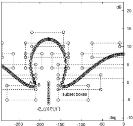
and phase2 ½360;0;with the grid resolution 108and 5 dB in the Nichols chart. The resulting bound, according to the algorithm above as implemented in Qsyn is marked by ‘A’ in Figure 7. Smaller search sets are now found around the computed course bound, marked as ‘subset boxes’ in Figure 7. Within these, the bound is computed with a resolution of 38and 1 dB. The resulting refined bound points are denoted by rings and the label ‘B’.

Note also in Figure 7 the ringed straight-line template with the labelPnomðjÞfPiðjÞ1gwhich denotes the template of plant inverses multiplied with PnomðjÞ:Its nominal is obviously the point1 (1808;0 dB). The rings denote the computed template points. The significance of this template is as follows: it is clearly seen in the tolerance specification (15)–(17) thatG¼ P1

i ;8i; would not satisfy the specification. Hence, the pointsP1

i Pnom;8i;will belong to the infeasible part of the complex nominal open loop plane (Lnom-plane), i.e. on the ‘forbidden’ side of the bound. The template PnomðjÞfPiðjÞg1 thus indicates which side of the bound is infeasible.

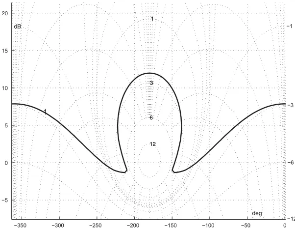
The final Horowitz–Sidi bound is also shown in Figure 8. Note that Horowitz’s original bound computation algorithm (Algorithm 1) would not have rendered correctly the ‘cusp’-like

Figure 7. A snapshot from the monitor screen of a bound computation inQsyn, displayed in the Nichols

chart of the complex Lnom-plane. ‘A’ denotes the bound marked by}only, found with the coarse grid

resolution (108;5 dB). ‘B’ denotes the refined bound, marked by}together with bold face ringso, found

shape of the bound at phases½150;1378;and hence might have resulted in a too conservative feedback regulator design.

6.2. Example

In Reference [21] an efficient bound computation algorithm is presented, see also references quoted therein. For the fourth-order aircraft example in Section 5 in Reference [21] a tracking bound for 0.1 rad/s is computed. Unfortunately, Table 2 in that paper is lacking, where the computational statistics were to be found. Our bound computation command cbnd in Qsyn

needed 2.484 s on a 1.86 GHz Pentium M computer to compute the same bound, based on a template consisting of 461 boundary points computed with the recursive grid I algorithm above with a resolution of (18;1 dB). The resulting bound had also the resolution (18;1 dB). Note that the commandcbndalso reads the template and specification files, presents graphical data as in Figure 7, and writes the bound data into a file, in addition to computing the bound itself.

7. CONCLUSIONS

The main advantage of the proposed Recursive Grid methods is the fact that it is possible to determine the required resolutions a priori. We have tested the recursive grid method for template computation on numerous examples and found the computational savings relative to

0 0

5 10 15 20

12 6 3 1 1

3

6

12

dB

deg

1

Figure 8. The final Horowitz–Sidi bound in Example 6.1 as computed inQsynwith resolution (38;1 dB),

the ‘brute force’ equidistant grid method to be substantial, typically between 50 and 95%. The recursive Horowitz–Sidi bound computation method gives a correct bound within the desired resolution, for all types of templates and specifications.

ACKNOWLEDGEMENTS

Particularly warm thanks are due to Isaac Horowitz’s former collaborator Dr Linda Neumann of El-Op Electro-Optics Ind. Ltd., Rehovot, Israel who wholeheartedly supported our effort to realize the QFT

design softwareQsyn}the Toolbox for Robust Control Systems Design for use with Matlab, and who

collaborated with us in many scientific, computational and application projects. The anonymous reviewers are acknowledged for their very useful inputs that made it possible to improve the paper considerably.

Supported by NUTEK Grant No. 9156700, the Fund for the promotion of research at the Technion– Israel Institute of Technology, and the European Union Marie Curie Transfer of Knowledge Program.

REFERENCES

1. Horowitz IM, Sidi M. Synthesis of feedback systems with large plant uncertainty for prescribed time domain tolerances.International Journal of Control1972;16:287–309.

2. Yaniv O, Horowitz IM. A quantitative design method for mimo linear feedback-systems having uncertain plants.

International Journal of Control1986;43(2):401–421.

3. Horowitz IM, Yaniv O, Neumann L. Flight control design with uncertain parameters.Technical Report AFWAL-TR-83-3036, Wrigth-Patterson Air Force Base, OH 45433, U.S.A., September 1983.

4. Gutman P-O, Neumann L. Horpac}a program for robust control systems design.Proceedings of the IEEE Control Systems Society 2nd Symposium on Computer Aided Control Systems Design, Santa Barbara, California, 1985. 5. A˚stro¨m KJ. Computer aided modeling, analysis and design of control systems}a survey.IEEE Control Systems

Magazine1983;3(2):4–16.

6. Yaniv O, Chait Y, Borgehesani C. The quantitative feedback toolbox for Matlab.Proceedings of ROCOND 97, Budapest, Hungary, 25–27 June 1991. IFAC.

7. Sating RR. Development of an analog MIMO Quantitative Feedback Theory (QFT) CAD package.M.S. Thesis, AFIT/GE/ENG/92J-04, Air Force Institute of Technology, Wright Patterson AFB, OH, 1992.

8. Houpis CH, Sating RR. MIMO QFT CAD Package (Ver.3).International Journal of Control1997;7(6):533–549. 9. Houpis CH, Rasmussen SJ, Garcia-Sanz M.Quantitative Feedback Theory:Fundamentals and Applications. A CRC

Press Book, Taylor & Francis: Florida, 2006.

10. Gutman P-O, Baril C, Neumann L. An algorithm for computing value sets of uncertain transfer functions in factored real form.IEEE Transactions on Automatic Control1994;39(6):1268–1273.

11. Gutman P-O.Qsyn}the Toolbox for Robust Control Systems Design for use with Matlab,User’s Guide and Reference Guide. Copyright: Per-Olof Gutman, 1996. Manuals downloadable from http://www.math.kth.se/optsyst/research/ 5B5782/index.html.

12. Cohen B. A program for computer aided design of robust control systems.Master’s Thesis, Faculty of Agricultural Engineering, Technion, Haifa, Israel, 1994.

13. Cohen B, Nordin M, Gutman P-O. Recursive grid methods to compute value sets for transfer functions with parametric uncertainty.Proceedings of the 1995 American Control Conference, vol. 5. IEEE: Philadelphia, 21–23 June 1995; 3861–3865.

14. Horowitz IM.Quantitative Feedback Design Theory(QFT). QFT Publications: Boulder, Co., U.S.A., 1993. 15. Bailey FN, Panzer D, Gu G. Two algorithms for frequency domain design of robust control systems.International

Journal of Control1988;48(48):1787–1806.

16. Yaniv O. Quantitative Feedback Design of Linear and Nonlinear Control Systems. The International Series in Engineering and Computer Science, vol. 509. Springer: Berlin, 1999.

17. Moreno JC, Ban˜os A, Montoya FJ. An algorithm for computing qft performance bounds. In Petropoulakis L, Leithead WE (eds).Proceedings of the 3rd International Symposium on Quantitative Feedback Theory and other Frequency Domain Methods and Applications, Brighton, England, 21–22 August 1997.

18. Brown M, Petersen IR. Exact computation of the horowitz bound for interval plants.Proceedings of the 30th IEEE Conference on Decision and Control, vol. 3. Brighton, England, 11–13 December 1991; 2268–2273.

20. Rodrigues JM, Chait Y, Hollot CV. A new algorithm for computing qft bounds.Proceedings of the 1995 American Control Conference, vol. 6. Seattle, Washington, 21–23 June 1991; 3970–3974.

21. Nataraj PSV. Computation of qft bounds for robust tracking specifications.Automatica2002;38(2):327–334. 22. Bailey FN, Hui C-H. A fast algorithm for computing parametric rational functions. IEEE Transactions on

Automatic Control1989;34(11):1209–1212.

23. Fu M. Computing the frequency response of linear systems with parametric perturbations.Systems and Control Letters1990;15:45–52.

24. Ackermann J.Robust Control: Systems with Uncertain Physical Parameters. Springer: Berlin, 1975.

25. Rantzer A, Gutman PO. An algorithm for addition and multiplication of value sets of uncertain transfer functions.

Proceedings of 30th CDC.Brighton, England, 1991; 2111–2115.

26. Ballance DJ, Hughes G. Survey of template generation methods for quantitative feedback theory.Proceedings of the 1996 UKACC International Conference on Control. Part 1. IEE Conference Publication, vol. 427/1. IEE: Stevenage, England, 2–5 September 1996; 171–174.

27. Chen W, Ballance DJ. Plant template generation of uncertain plants in quantitative feedback theory.Journal of Dynamic Systems,Measurement and Control(ASME) 1999;121(2):358–364.

28. Cervera J, Ban˜os A, Horowitz IM. Computation of siso general plant templates. In Proceedings of the 5th International Symposium on QFT and Robust Frequency Domain Methods, Mario Garci´a-Sanz (ed.). Universidad Pu´blica de Navarra, Pamplona, Spain, 2001; 247–254.

29. Garcia-Sanz M, Vital P. Efficient computation of the frequency representation of uncertain systems.

4th International Symposium on Quantitative Feedback Theory and Robust Frequency Domain Methods, Durban, South Africa, August 1999; 117–126.

30. Boje E. Finding nonconvex hulls of QFT templates.Journal of Dynamic Systems,Measurement and Control(ASME) 2000;122(1):230–232.

31. Gutman P-O, Neumann L, A˚stro¨m KJ. Incorporation of unstructured uncertainty into the horowitz robust design method.Proceedings of IEEE International Conference on Control and Applications,ICCON’89, Jerusalem, Israel, 3–6 April 1989.

32. Kahaner D, Moler C, Nash S.Numerical Methods and Software. Prentice-Hall: Englewood Cliffs, NJ, 1989. 33. MATLAB 6.5, High Performance Numeric Computation and Visualization Software. The MathWorks Inc.:

Cochituate Place, 24 Prime Park Way, Natick, MA.