Evaluating and improving the passenger punctuality of a timetable

(1)

Master thesis - Applied Mathematics

Evaluating and improving

the passenger punctuality

of a timetable

Marjan Nelis

Faculty of Electrical Engineering, Mathematics & Computer Science (EEMCS)

Department of Discrete Mathematics and Mathematical Programming (DMMP)

Supervisors:

Prof. dr. M.J. Uetz (University of Twente)

Dr. G. Mar ´oti (Nederlandse Spoorwegen)

Assessment committee:

Prof. dr. M.J. Uetz (University of Twente)

Dr. G. Mar ´oti (Nederlandse Spoorwegen)

Dr. ir. W.R.W. Scheinhardt (University of Twente)

(2)

(3)

Abstract

(4)

(5)

1 Introduction

This first chapter provides an introduction to several subjects which are essential for a full understanding the context of the problem at hand. Firstly, the Dutch Railways and passenger punctuality are briefly introduced in Section 1.1 and Section 1.2 respectively. This is followed by a description of delays in the operation and a relevant model in Section 1.3 and Section 1.4. In Section 1.5, the problem description and research question are presented. Finally, the outline of the thesis is given in Section 1.6.

1.1 Dutch Railways and their performance

In the Netherlands, the train is a common way of traveling. The rail network has a length of more than 3000 kilometers of track and is used daily by over 1.1 million passengers. It is one of the busiest railway networks of Europe. There are several companies responsible for the train operations, includingNederlandse Spoor-wegen(in English, Dutch Railways, or abbriviated as NS), Arriva, Connexxion and Syntus. The largest operator is NS; which is responsible for operation the passenger trains on the Main Rail Network (HRN). NS aims to deliver high quality services for the passengers including a reliable timetable, sufficient and comfortable materials and adequate response to disturbances (CBS, 2016; NS, 2016; ProRail, 2017).

NS is held accountable for its performance to the Dutch government. The performance is measured by a set of Key Performance Indicators (KPIs) such as general customer opinion, passenger punctuality and seating chance. For all the KPIs, target values for the upcoming years are recorded in an agreement with the Dutch government. If the target values are not achieved, there could be negative consequences for NS, such as fines or even losing its transport concession.

1.2 Passenger punctuality

Passengers punctuality is a KPI, which gives a measure for the reliability of the NS’ services. It is defined as the percentage of passengers for whom the journey, in terms of travel time, was successful. There are three variations of passenger punctuality stated in the agreement of NS with the government (NS, 2016).

• Passenger punctuality 5 minutes HRN; i.e. the percentage of passengers arriving at their destination within 5 minutes of their promised arrival times. Here the punctuality is only measured for journeys on the main rail network.

• Passenger punctuality 15 minutes HRN; i.e. the percentage of passengers arriving within 15 minutes of their promised arrival times. Here the punctuality is only measured for journeys on the main rail network.

• Passenger punctuality 5 minutes High Speed Line (HSL); i.e. the percentage of passengers arriving within 5 minutes of their promised arrival times. Here the punctuality is only measured for journeys on the high speed line.

For the trains, a schedule is made which includes the planned arrival and departure times at train stations, this schedule is denoted as thetimetable. The actual arrival and departure times in the execution of the timetable may differ from the planned times. Therealization datacontains the actual arrival and departure times of the trains, from which the delay of each passenger can be derived. The passenger punctuality is calculated by dividing the number of passengers whose delay is smaller than the threshold of time (either 5 or 15 minutes) by the total number of passengers.

For each of the three passenger punctuality KPIs, Table 1.1 gives an overview of the results of previous years and the target values for 2019. Up until 2017, none of these KPIs have reached their target value. In April 2017, NS made the headlines due to their poor performance on the HSL. NS received a fine of e500.000 from the State Secretary of the Ministry of Infrastructure and Environment, because they had not reached the bottom value for the 5 minute passenger punctuality on the HSL in 2016 (Dijksma, 2017).

(8)

Table 1.1:Overview of the passenger punctuality KPIs (NS, 2016).

5 min. HRN 15 min. HRN 5 min. HSL

Realization 2015 90.0% 97.0% 81.8% Realization 2016 90.5% 97.1% 80.5% Progression value 2017 90.5% 97.0% 82.5% Target value 2019 91.3% 97.3% 84.3%

services. Therefore, improving the reliability of the trains is a crucial point of focus for the following years in order to achieve the target values in 2019.

1.3 Delays in the operation

In order to improve the future passenger punctuality KPIs, analysis of the root cause, delayed trains, is required. The trains either caused the delayed arrivals of the passengers directly or induced missed transfers. Two types of delays are defined:

• Primary delaysfollow directly from disturbances that occur during the execution of the timetable. These disturbances can have many sources, either from within the railway system or its environment. As a consequence, processes, such as movements and stops, take longer to execute than planned and delays may occur.

• Secondary delays, also called knock-on delays, are delays caused by earlier delays in the system. In the busy railway network of the Netherlands, the major part of delays are secondary delays.

The design of the timetable influences the impact of both primary and secondary delays on the system by the following reasoning. A movement of a train between locations and the dwelling of a train at a station is noted as a process. Each process within the timetable has a certaintechnically minimum process time, which is the minimal time that is necessary to execute the process. On top of these minimum process times,

time supplementsare added. This additional time is scheduled in the timetable to (partially) absorb delays and reduce knock-on delays. The location and magnitude of the time supplements affects the performance of the timetable (Vromans, 2005).

1.4 Stochastic Optimization Model

The Stochastic Optimization Model (SOM) by Kroon et al. (2008) is designed to redistribute the time supplements in a timetable to improve its performance. Kroon et al. (2008) improve the robustness of the timetable by minimizing the expected train delay. By minimizing the average weighted train delay the authors aim to achieve improvement with respect to train punctuality. Therefore, SOM could be a useful tool to improve the passenger punctuality in our situation.

An improvement in train punctuality could mean improvement in passenger punctuality, but this can not be guaranteed as stated by Nielsen et al. (2009). In Section 2.4 it is shown in several cases that the passenger punctuality can be higher, lower or equal to the train punctuality depending on the delays of the trains.

1.5 Problem definition

(9)

supplement allocation. These circumstances make it is essential to evaluate the performance of timetables beforehand under similar conditions.

The first goal of this thesis is filling one of these gaps by developing and test a model which can evaluate the performance of timetables under similar conditions. Such a model can provide a measure for the passenger punctuality and will contribute to a simple method of comparing timetables and analyzing where the supplement needs to be allocated for the best performance, without actually executing the timetables. To recreate realistic conditions in such a model, for both the realization data of the trains and the data of the passengers, proper assumptions and predictions have to be made based on data that is available.

With the evaluation model, a second goal is set for this thesis: improve a given timetable with respect to passenger punctuality. SOM will be used to reach this goal. Instead of evaluating the expected average weighted train delay, the performance of a timetable improved by SOM should be evaluated by the new evaluation model. This lead to the following main research question:

How can timetables be improved using passenger punctuality as measure?

In order to answer the main research question properly, several sub questions are formulated. The research is divided into two parts. The first part focuses on developing a measuring tool of passenger punctuality for a given timetable. This part starts with a review about passenger punctuality. The first and second sub questions for this part are therefore formulated as follows:

1. How is passenger punctuality calculated? What input is necessary?

2. How can passenger punctuality be used to develop a new performance measure for an unrealized timetable?

In the second part of the research, focus is on improving timetables using passenger punctuality as perform-ance indicator. SOM will be used as the base of the proposed model. In this part the third and fourth sub questions will be answered:

3. What is SOM and what are its limitations?

4. How can passenger punctuality be used in SOM to improve timetables?

1.6 Thesis outline

(10)

2 Calculation of passenger punctuality

In Chapter 1, passenger punctuality is defined as the percentage of passengers which arrive at their final destination within a certain threshold of time from the promised arrival time. This chapter explains how the passenger punctuality is calculated by NS, and we refer to this system asNS’ system. NS’ system functions as a guideline for the proposed evaluation model in Chapter 4; the evaluation model simulate NS’ system for any given timetable to obtain a measure for the passenger punctuality.

To introduce the terminology, we start with an example of the journey of a single passenger in Section 2.1. In Section 2.2, the modules in NS’ system are explained. Some of the assumptions made in the calculation are briefly discussed in Section 2.3. In Section 2.4, the difference between train punctuality and passenger punctuality is shown in several theoretical situations. Finally, the chapter is concluded and summarized in Section 2.5.

2.1 Example case

To illustrate how the delay of each passenger is determined, this section provides an example with a single passenger. In the Netherlands, theOV-chipkaart is the obligatory payment method for public transport. Passengers check in with this card at their departure station and check out at their destination station. From the data of the Check Ins (CI) and Check Outs (CO), abbreviated to CICO data, the cost of the journey is determined. The same CICO data is used for the calculation of the punctuality of the passengers.

2.1.1 From CICO data to travel promise

The particular passenger in this example travels from station Nuth to station Schiphol Airport in the morning of September 27th. The journey produces the following CICO data, see Table 2.1.

Table 2.1:The CICO data of the passenger.

CI station Nuth

CI date and time 27 September 2016 07:35 CO station Schiphol Airport

CO date and time 27 September 2016 10:40

The first step is to find the path the passenger followed: to determine which trains the passenger used in its journey. Taking into account the standardcheck in marginof 1 minute (due to the distance between the check in poles and the platforms), the departure time will be 07:36. The passenger wants to travel as fast as possible from Nuth to Schiphol Airport after 07:36. For this, the travel planner of NS is utilized.

The departure time 07:36, the CI station Nuth and the CO station Schiphol Airport are offered to the

travel planner. The travel planner provides several travel possibilities, each with different departure times or different paths. These travel possibilities are denoted astravel options. In Figure 2.1, the option which promises the earliest arrival at the destination is displayed. This travel option is further on denoted as the

travel promiseof the passenger and provides the promised arrival time of the passenger.

2.1.2 Realization of the travel promise

The next step is analyzing the journey. The travel promise can be divided into threetravel partswhere each part is a different train, the parts are separated by the transfers. The travel promise provided the train data as they were planned in the timetable. From the realization data of the trains that morning, we obtain the following data about the travel parts, as represented in Table 2.2.

• Travel part 1 had a arrival delay of 6 minutes, its arrival time is 08:15.

• Travel part 2 had a departure delay of 5 minutes, its departure time is 08:18.

(11)

[image:11.595.194.397.133.433.2]

Figure 2.1:The selected travel option: the travel promise (NS, 2017).

Table 2.2:Overview of the three travel parts.

Departure station Departure time Arrival station Arrival time

1 Nuth 07:54 Sittard 08:09+6

2 Sittard 08:13+5 Utrecht 09:51

3 Utrecht 09:58 Schiphol Airport 10:27

For each travel part, the departure delay is checked. If the departure delay is larger than 15 minutes, the journey is rescheduled. In this example none of the travel parts experience such a delay. What remains is checking the transfers. If a transfer is missed, the journey has to be rescheduled as well. The travel promise of this passenger contains the next two transfers.

• Travel part 1 arrived at 08:15 at Sittard, travel part 2 departed from Sittard at 08:18. With 3 minutes of changeover time this was a successful transfer.

• In Utrecht travel part 2 arrived without delay and part 3 departs without delay. The transfer was executed as promised, and hence, successful.

[image:11.595.135.460.488.539.2]

(12)

2.2 Modules of the NS’ system

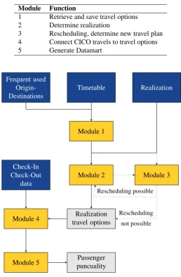
[image:12.595.167.426.215.610.2]

The system, which calculates the passenger punctuality, determines the delay and therefore the punctuality of all passengers at once. The algorithm behind the calculation of passenger punctuality follows the over-view chart depicted in Figure 2.2. The blue blocks represent the input data of the system, the yellow blocks represent the modules in which the calculations take place and the remaining light gray blocks represent output of the modules. In Table 2.3, a summary is given of the modules. The function of each module is explained in the Section 2.2.1 to Section 2.2.5.

Table 2.3:Modules of the NS’ system. (van der Berg, 2015)

Module Function

1 Retrieve and save travel options 2 Determine realization

3 Rescheduling, determine new travel plan 4 Connect CICO travels to travel options 5 Generate Datamart

Frequent used Origin-Destinations

Timetable Realization

Module 1

Module 2 Check-In

Check-Out data

Module 3

Module 4 Realization travel options

Module 5 _puncualityPassenger

Rescheduling

not possible Rescheduling possible

Figure 2.2: A simplified visualization of the system which calculates the passenger punctuality. The blue blocks represent the input data of the system, the yellow blocks represent the modules in which the calculations take place and the remaining light gray blocks represent output of the modules. (Wolters, 2016; van der Berg, 2015)

2.2.1 Module 1: Retrieve and save travel options

(13)

First, the module determines the list of frequently usedOrigin-Destinationcombinations (ODs). The system only considers ODs which are frequently used by passengers, ODs which are never or barely used are neglected. The list of frequent ODs is determined based on the CICO data from the previous 100 days. An OD is taken into account if it appear at least 100 times over the last 100 days and on at least 20 different day over the last 100 days. The list is updated four times a year. This way the system includes new stations and neglects stations that are no longer used. It reduces the number of ODs by approximately 70% while preserving over 98% of the journeys (van der Berg, 2015).

Once the frequent ODs are determined, the corresponding travel options are retrieved from the journey planner. The request to the journey planner results in a large number of options.Each unique travel option is identified and saved for the next module.

2.2.2 Module 2: Determine realization

Module 2 determines the realization of all travel options through their corresponding travel parts. This is similar to the process in Section 2.1.2 where the travel is analyzed. The realization is determined with the actual departure and arrive times of the train at stations, this data is denoted as therealization data. For each travel part is determined:

• if the train departed and at what time the train departed,

• if the train arrived and at what time the train arrived.

Once the realization of the travel parts is known, the realization of the travel options is determined. Travel options with missed transfers or severe delays require rescheduling before the delay can be determined. These travel options are sent to module 3 and this module returns the rescheduled travel options to module 2.

For every (rescheduled) travel option the realized arrival times are determined by the actual arrival time of the final travel part, like the example case in Section 2.1.2. The outcome of module 2 is a database with every travel option combined with the realization data.

2.2.3 Module 3: Rescheduling

Module 3, as mentioned in Section 2.2.2, takes care of travel options that require rescheduling. These are the travel options with missed transfers or with severe delays. Module 3 returns the rescheduled option to module 2 were its realization is determined.

In the current system, no rescheduling takes place; the checkout time minus a predetermined margin is used to estimate the realized arrival time. This makes the whole rescheduling process easier, but less accur-ate due to the behavior of the passengers. Passengers may remain longer at a station than the predetermined margin, this results in an overestimation of the delay.

2.2.4 Module 4: Connect CICO data to travel options

In module 4, the passengers from the CICO data are connected to the travel options in order to determine the delay of each passenger. The CICO data contains the origin, the destination, check-in time and check-out time of every trip made. Based on this information, a travel option is selected for each passenger, which is denoted as the travel promise of the passenger. This process corresponds with Section 2.1.1 of the example case, where the fastest journey from Nuth to Schiphol Airport was selected.

The connection of the CICO data to the travel options happens in such a way that the option with the earliest arrival time is selected. This happens according to the following procedure:

i. From the check-in time plus the check-in margin, all travel options of the next hours are collected. The check-in margin is equal to the specific check-out margin per station.

ii. All travel options for which a quicker alternative exists are deleted.

iii. Based on the departure time, the first option after the check-in time is selected as was determined by the journey planner.

(14)

2.2.5 Module 5: Generate Datamart

In the fifth and last module, the data of the previous modules is exported in the correct format for NS. For each OD combination, the number of travels per day and the delay category is saved to determine the passenger punctuality KPIs.

For all ODs the number of passengers is counted and determined if their delay lies within the threshold. There are two KPIs with a threshold of 5 minutes and one with a threshold of 15 minutes. All measurements with a delay less than the threshold is divided by the total number of measurements resulting in the passenger punctuality.

2.3 Assumptions in the calculation

In the method of calculating passenger punctuality, 22 assumptions are made (see Table A.1 in Appendix A). These assumptions are about the behavior of the passengers and the correctness of the data. We are not going to elaborate on all these assumptions here. Note, however, that some of the assumptions made in the calculation are also used in the proposed evaluation model that will be presented in Chapter 4. The fourth item in Table A.1 provides a clear example; this assumption states that passengers want to go as quickly as possible from A to B. Therefore is chosen for a shortest path approach in the new evaluation model to determine travel promises.

2.4 Train punctuality versus passenger punctuality

In order to show that the passenger punctuality can differ form the train punctuality, two theoretical situ-ations are sketched in Section 2.4.1 and Section 2.4.2. The train punctuality is defined as the percentage of trains which arrive at a station with a delay less than the given threshold. By adapting the train delays, the passenger punctuality can turn out to be higher, lower or equal to the train punctuality in each situation. An overview of the results is given in Section 2.4.3

2.4.1 A journey with a transfer

For the first situation, the network of Figure 2.3 is considered. It consists of three stations, two trains and one passenger. The passenger travels fromAviaBtoCand transfers from traint1to traint2in stationB.

The transfer time in the schedule is determined as the walking time between the trains at stationB plus 2 minutes buffer time. The thresholds for the passenger and train punctuality is set on 5 minutes. Thus the trips are considered unpunctual if their delay is 5 minutes or more. Furthermore,t2does not wait ont1.

A B C

t1 t2

Figure 2.3:The network with a transfer.

In each of the following four cases, the train delay is altered in order to create scenarios with different train and passenger punctualities.

Case I

First, consider the trivial case where both trains have no delay. In this case, the transfer is successful and the passenger arrives atCwith no delay. Both train and passenger punctuality are 100%.

Case II

Assumet1arrives atBwith a delay of 3 minutes andt2departs fromBas planned. The passenger cannot

make the transfer tot2and will not arrive at stationC. Both trains arrive within the threshold of 5 minutes at

(15)

Case III

Assume that both trains are delayed. Train 1 arrives atB with a delay of 5 minutes and train 2 departs with a delay of 4 minutes fromB and arrives atC with the same delay. The passenger is able to transfer successfully at stationBsince the transfer time is the walking time plus one minute buffer time. Following the punctuality threshold of 5 minutes, train 1 is considered unpunctual and train 2 is considered punctual. The train punctuality is 50%. The passenger arrives at station C with 4 minutes delay, the passenger punctuality is 100%.

Case IV

Finally, consider for this network the situation where train 1 has no delay and train 2 has a delay of 6 minutes at both departure and arrival station. The transfer is made successfully. The train punctuality is 50% since the delay of train 2 is larger than the threshold. The passenger arrives with a delay of 6 minutes at stationC, the passenger punctuality is 0%.

2.4.2 A journey without transfers

The second situation is slightly different from the first. It is illustrated in Figure 2.4. Here, we consider three stations, one train, and one passenger. The train departs from stationAand moves via stationB to stationC, the passenger travels fromAtoCwith this train. The differences in the following two cases are due to the measure points of the train delay. The train delay is measured at each arrival, that is in stations BandCin this situation while the passenger punctuality is only measured at the end of the passengers’ journey.

A B C

t1 t1

Figure 2.4:The network without a transfer.

Case V

Assume that the train arrives on time atBand with a delay of 6 minutes atC. The train has, with its two measure points a punctuality of 50%. The passenger arrives with a delay of 6 minutes at its destination. Therefore, the passenger punctuality is 0%.

Case VI

(16)

2.4.3 Overview of the cases

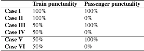
For the first situation with a transfer, the four cases show the importance and the influence of the transfers on the punctuality. A train punctuality of 100% does not guarantee a passenger punctuality of 100% and vice versa.

[image:16.595.175.416.227.313.2]

Since a large part of the passengers travels without any transfers, a situation without transfers is also discussed. Case V and VI show that, even in a situation without transfers, the passenger punctuality and train punctuality can be different due to the fixed measure points for the train punctuality.

Table 2.4: An overview of the punctualities is the situation with transfer (cases I-IV) and without transfer (cases V-VI).

Train punctuality Passenger punctuality Case I 100% 100%

Case II 100% 0%

Case III 50% 100%

Case IV 50% 0%

Case V 50% 100%

Case VI 50% 0%

2.5 Summary

The main subject of this chapter is passenger punctuality. Using an example case, the punctuality was determined for a single passenger. This is followed by the elaboration of the NS’ system, which calculates the passenger punctuality of all passengers. The system consists of the five modules:

• The first module determines all possibletravel optionsin the timetable. These are the possible jour-neys passengers can use to travel between anOrigin-Destination(OD) pair.

• The second module combines the realization data with the travel options to determine its delay, if possible.

• The third module reschedules the journey in case of large delays or missed transfers, the results of the third module are returned to module 2. The current system does not use dynamic rescheduling, instead the check out times are used to estimate the delay.

• The fourth module connects the passengers to travel option using theirCheck-InandCheck-Out data

(CICO data).

• The fifth and last module categorizes the delays of the passengers and determines the values of the passenger punctuality KPIs.

(17)

3 Stochastic Optimization Model

The Stochastic Optimization Model (SOM), as shortly addressed in Chapter 1.4, is designed to redistribute the time supplements of a given timetable to improve its robustness against small disturbances. This im-provement is established by minimizing the expected weighted train delay. SOM is created by Vromans (2005) and improved by Kroon et al. (2008). The improved model of Kroon et al. (2008) is implemented by the company Niks et al. (2015) and this implementation will be used in Chapter 6 to improve timetables. In Section 3.1, SOM is described as defined by Kroon et al. (2008). Section 3.2 provides relevant implementation details of the implemented model.

3.1 Model description

SOM is divided into a timetabling part and a simulation part. The timetabling part determines the timetable and shows similarity with the well-known Periodic Event Scheduling Model by Serafini and Ukovich (1989). The simulation part runs independent realizations of the timetable, subject to stochastic primary disturbances, in order to evaluate the expected train delay of the the timetable.

Since SOM only considers small disturbances, we have the following assumptions: The first assumption is that the train order on the tracks is determined by the initial timetable and cannot be modified. Moreover, all planned connections between train are assumed to be maintained in the realizations.

3.1.1 Notation

A timetable consists ofprocesses that have to be executed. For example, the movement of a train from one station to another, the dwelling period at a station, safety processes such as headway time between consecutive trains on the same track, and commercial processes like planned passenger transfers. The beginning and completion of a process are calledevents. The events correspond with the departure, arrival or crossing of a certain train at a given location.

NS uses acyclic timetablewith a cycle timeTof one hour for their operations. Cyclic timetabling means that the timetable of longer periods can be created by copying a timetable of a single cycle. Therefore, the timetabling part of SOM only uses one cycle, theOne-Hour Timetable(OHT), as input.

In an OHT, the set of processesP and the set of eventsEare defined. For each processp ∈ P, the eventsb(p) ∈ E andc(p) ∈ E denote the beginning and completion events, respectively. Furthermore, parametermpdenotes thetechnically minimum process timeof processp∈P, that is the minimum time

necessary to execute processp.

The planned time of an eventeis denoted by the parameterVe. This parameter states the minute in

the hour on which eventeis planned. The beginning and completion time of a processpis denoted by Vb(p)andVc(p), respectively. If a process is completed within an hour, the inequalityVb(p)< Vc(p)holds.

Otherwise, if a process crosses the end of an hour,Vb(p) > Vc(p)holds. To separate these two cases, the

binary parameterQp is introduced. This parameter records whether or not the process crosses the end of

the hour. This results in the following definition:

Qp= (

0 ifVb(p)< Vc(p)

1 ifVc(p)< Vb(p)

In the improved timetable, the event times and time supplements are the decision variables. The new event time of eventeis denoted byveand the time supplement on a processpis denoted by the decision variable sp. The improved event times are not restricted to the time interval[0, T −1]in order to prevent unwanted

restrictions. The final event times in the optimized timetable are obtained by transferring the initial obtained final event times back to the interval[0, T −1].

SOM evaluates expected average train delay of the timetable under construction throughRsimulations. In each simulation, the OHT is expanded to a day ofHconsecutive hours and the timetable is subject to a priori selected independent stochastic primary disturbances. The variable˜ve,r,hdenotes the planned event

time of eventein hourhof simulationr. The disturbance parameterδp,r,hdenotes the primary disturbance

(18)

so each process is subject to one primary disturbance. The decision variableDe,r,h denotes the delay,

including both primary and secondary delays, on eventein hourhof simulationr. Furthermore, the train delay is only measured at the arrival events, the set of arrival events is denoted byEa.

3.1.2 Timetabling part of the model

Using the notation as introduced in the previous section, the constraints of the time tabling part of SOM are formulated.

mp+sp=vc(p)−vb(p)+Qp·T forp= 1, . . . , P. (1)

The right-hand side of equation (1) describes the time difference between the variables of the planned completion time and begin time of processp, here the possible crossing of the end of the hour is taken into account. Thus the right-hand side is the total planned process time of processpin the new timetable. The total planned process time is equal to the left-hand side: the technically minimum process timemp, a

parameter, plus the added time supplementspon processp.

The added time supplements are non-negative, therefore the parametermpis a lower bound for the total

planned process time as described in the right-hand side of (1). Furthermore, there may be a upper bound upspecified for processp. This results in the following constraints:

mp≤vc(p)−vb(p)+Qp·T ≤up forp= 1, . . . , P.

Lete1denote the first planned event in an hour on a location ande2denote the last planned event in an hour

on the same location. To guarantee that the obtained timetable can be transferred back to the time interval

[0, T −1], the time difference betweene1ande2 should not exceed the cycle timeT. This is important

since the event times are not restricted to the time interval, as explained earlier.

0≤ve2−ve1 ≤T −1.

The following constraints set a maximum amount of time supplements on selected subsets of processes. Let there beN subsetsA1, . . . , AN selected, each subsetAnis connected to the maximum amount of time

supplementSnto be allocated in the corresponding subset.

X

p∈An

sp≤Sn, forn= 1, . . . , N.

Finally, delaysDe,r,hare considered non-negative and integrality constraints are imposed on the planned

event timesveand the variables time supplementssp.

3.1.3 Simulation part of the model

In the simulation part of SOM, days ofH consecutive hours are simulated. A processpwithQp = 0has Vb(p)< Vc(p), thus it is planned within a single hour and ends in the hours with the same index as the hour

it started in. A processpwithQp= 1hasVc(p)< Vb(p), it ends in the hour with an index higher than the

hour it started in: processpwithQp = 1starts in hourhof realizationratv˜b(p),r,h, this process ends at

˜

vc(p),r,h+1

The following constraints simulate the effects of both primary and secondary delays. The event times of the processes are linked to the technically minimum process times and primary disturbances. The primary delays are directly simulated by adding the disturbancesδp,r,h. The secondary delays are indirectly

simu-lated: they follow from interacting processes between trains.

mp+δp,r,h≤v˜c(p),r,h+Qp−v˜b(p),r,h forp= 1, . . . P; r= 1, . . . , R; h= 1, . . . , H. (2)

Furthermore, departure events are not allowed to occur too early. Here the set of departure events is denoted byEd.

(19)

The delay of the arrival events is determined by subtracting the simulated event time from the planned event time, as presented in the following constraints:

˜

ve,r,h−(ve+h·T)≤De,r,h ∀e∈Ea; r= 1, . . . , R; h= 1, . . . , H.

3.1.4 Objective function

The objective of SOM is to minimize the average weighted delays of the trains. The objective is defined by Kroon et al. (2008) as

minimize X

e∈Ea R X r=1 H X h=1

weDe,r,h/(|Ea| ·R·H). (3)

3.2 Implementation by ORTEC

In Chapter 6, SOM is used to improve timetables. We use SOM with both the implemented version of the objective function by Niks et al. (2015) as well as with an customized objective function. Therefore the implementation of the objective function by ORTEC is introduced in this section.

The objective function in the implementation by ORTEC is different from the objective function as presented in (3). In order to explain the differences, several new notations are introduced. Firstly, the subset of arrival events that are located at a predetermined measure points is denoted byEm. Secondly, the subset

of arrival events for which is indicated in the input that extra weight must be added is denoted byEe.

Finally, besides the delay variableDe,r,han extra variableDMe,r,his introduced which indicates the delay

above a predetermined margin.

The objective function consists of eight differently weighted delays. The eight weighted delays are defined as follows:

WD1=w1·

X

e∈E R X r=1 H X h=1 DMe,r,h

|E| ·R·H, WD2=w3· X

e∈E R X r=1 H X h=1 De,r,h |E| ·R·H,

WD3=w3·

X

e∈Ea R X r=1 H X h=1 DMe,r,h |Ea| ·R·H

, WD4=w4·

X

e∈Ea R X r=1 H X h=1 De,r,h |Ea| ·R·H

,

WD5=w5·

X

e∈Em R X r=1 H X h=1 DMe,r,h |Em| ·R·H

, WD6=w6·

X

e∈Em R X r=1 H X h=1 De,r,h |Em| ·R·H

,

WD7=w7·

X

e∈Ee R X r=1 H X h=1 DMe,r,h |Ee| ·R·H

, WD8=w8·

X

e∈Ee R X r=1 H X h=1 De,r,h |Ee| ·R·H

,

The objective function in the implementation by Niks et al. (2015) is defined as

(20)

4 Evaluation model

In this chapter, the model is described that we have built to evaluate timetables. The goal of the evaluation model is to give a measure for the passenger punctuality. This measure is obtained by simulating the delays of passengers under small disturbances. The passenger punctuality is extracted from these delays. The evaluation model aims to remain as close as possible to NS’ system to determine passenger punctuality.

After a literature review in Section 4.1, the design of the evaluation model is stated and elaborated upon Section 4.2 to Section 4.6. The chapter is concluded in Section 4.7 by addressing several remarks concerning the evaluation model.

4.1 Literature review

Little research has been carried out that concerns modeling passenger delays. Landex (2008) and Nielsen et al. (2009) give an overview of passenger delay models and present their schedule-based route choice model (see Table 4.1). In the overview, the passenger delay models are categorized into generations. Landex (2008) and Nielsen et al. (2009) classify the simplest models as0th _generation_{models, these are models}

used by railway companies and not reported in international literature. Nielsen et al. (2009) created the descriptions of these models based on interviews with the railway companies. Since this generation of models does not use schedule-based routes, the 0th generation models are disregarded. We start with a description of models Landex (2008) and Nielsen et al. (2009) classified as the1st generationpassenger passenger delay models, followed by the2ndand3rdgeneration.

1st_generation

The first models, which use the schedule-based routes, are denoted as the1stgenerationpassenger delay models by Landex (2008). The core idea of these passenger delay models is that the passenger delay is modeled by calculating the optimal route in the planned timetable and the optimal route in the realized (potentially delayed) timetable. The passenger delay is calculated by taking the difference in time of the two routes. The optimality of the route in the realized timetable implies the assumption that passengers have knowledge of all present and future delays. This principle of passenger route choice is denoted as the

optimistic principle.

The advantage of the 1st_{generation passenger delay models is that they take in account the passengers’}

route choices. Another advantage is that the models can easily be applied by running the standard route choice model on the realized timetable. Moreover, the entire trip (including transfers) is examined by the model, in contrast to simpler models from the 0thgeneration.

The disadvantage, as noted before, is that the optimal route choice model, which is used in the realized timetable, assumes that the present and future delays are known to the passengers. This results in an under-estimation of the passenger delay compared with the reality, because in reality, passengers often become aware of the delay during their trip.

2nd_generation

The2nd_generation_{of passenger delay models uses a number of simulations of the timetable with empirical}

or simulated delay distributions. The passengers choose their optimal route in each of the simulations. This generation also assumes that passengers have knowledge of future delays, the results of the simulations lead to a route choice taking into account the expected delay distribution. Moreover, a large amount of memory is required as each route choice for each simulation has to be stored.

3rd_generation

(21)

• Pessimistic principle: Passengers may use the same route as planned, they do not act upon better routing opportunities along the route.

• Optimistic principle: The optimal path search is applied to determine the paths of the passengers in the realized timetable. This principle assumes that the passengers have knowledge about all present and future delay in the timetable and determine their optimal path accordingly.

The passengers in the 3rd_{generation model by Nielsen et al. (2009) reconsider their route if they experience}

[image:21.595.92.501.261.434.2]

a certain amount of delay. Moreover, if the desired route is no longer feasible due to delays, the passengers reconsider their route immediately. The reconsideration takes places at the point threshold is exceeded or the route is no longer feasible. This results in a more realistic model as compared to previous generations, but is more complicated to implement due to the rescheduling along the passengers’ journeys.

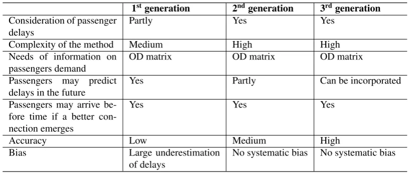
Table 4.1:Overview of the characteristics of the passenger delay models (Nielsen et al., 2009).

1st_generation ₂nd_generation ₃rd_generation

Consideration of passenger delays

Partly Yes Yes

Complexity of the method Medium High High Needs of information on

passengers demand

OD matrix OD matrix OD matrix

Passengers may predict delays in the future

Yes Partly Can be incorporated

Passengers may arrive be-fore time if a better con-nection emerges

Yes Yes Yes

Accuracy Low Medium High

Bias Large underestimation of delays

No systematic bias No systematic bias

4.2 Design of the evaluation model

The design choices of the evaluation model are mostly based on the design choices of NS’ passenger punc-tuality system, because that is the system we want to simulate. In Chapter 2, the necessary input of NS’ system is discussed. The only input data we have at our disposal is the timetable. The remaining input (fre-quent ODs, realization data, and CICO data) is not available, because these follow from the execution os the timetable. Alternative data must be used and that brings along limitations. Furthermore, the input of the simulations (disturbances) is chosen similar to the input of SOM. SOM evaluates the train delay using its own simulations, the evaluation model functions as a extension of SOM by evaluating passengers delay and punctuality in similar simulations. All assumptions, alternative approaches, and limitations are discussed in Section 4.7.

The modules of NS’ system return in the following way into the evaluation model:

• Firstly, all possible paths between any combination of train stations are determined using the original timetable and connected to passenger groups(see Section 4.3.2). These paths are denoted as the

nominal paths. This part corresponds with module 1 of NS’ system.

• Secondly, a realization is simulated by adding disturbance to the timetable and in this realization all possible paths are determined again and connected to the passenger groups. These paths are denoted as therealized paths. This procedure is similar to modules 2 and 3.

(22)

The next sections are organized as follows: Section 4.3 provides a description of the input data. Section 4.4 describes how this data is used to calculate the nominal paths of the passengers. The calculation of the realized paths is elaborated upon in Section 4.5. This is followed by the output of the model in Section 4.6. In Section 4.7, the limitations of the model are discussed.

4.3 Input data

The input of the evaluation model are the reference timetable, theOrigin-Destination(OD) matrix, and a passenger distribution over the day. The timetable is used to determine the nominal and realized paths of the passengers. The OD matrix and passenger distribution are used to recreate the frequent ODs and CICO data. Furthermore,passenger groupsare introduced simulate the passengers.

4.3.1 Reference timetable

The format of the reference timetable in the evaluation model is identical to the format used in SOM; they both use anOne-Hour Timetable(OHT). This makes it possible to apply both models on the same timetable. We start by repeating the definitions concerning timetables, note that the evaluation model uses a different notation than SOM.

A timetable consists ofeventsandprocesses, these are interpreted as follows. An event corresponds with the departure, the arrival, or a crossing of a given train at a given location. The processes of a train are either a movement between two locations or the dwelling at a station. Next to that, there are processes for safety and commercial issues, such as the headway restrictions between trains and transfer opportunities for the passengers.

The reference timetable is presented as acyclic timetable. Cyclic timetables specify a longer period as repeated copies of shorter periods or cycles. In the case of NS, such a short period is an hour, i.e. the cycle timeT = 60minutes. All data, events and processes, are only specified for a single hour, the OHT. The length to which the cyclic timetable is extended in the evaluation model is determined by the parameter H, this is the number of cycles in the extension. In this section, a distinction is made between events and processes of the cyclic timetable and the extendedlinear timetable, they are noted ascyclic events and processesandlinear events and processes, respectively.

The cyclic events are the basis of a timetable, they form the setE. The cyclic timetable πassigns the cyclic events to time instants in the cycle. The planned time of cyclic eventε ∈ E inπ satisfies

0≤π(ε)< T.

The cyclic events are connected and restricted through the cyclic processes. LetP denote the set of cyclic processes. The events with which the processes start and end are given. Furthermore,technically minimum process timesand the binary parameterQ(which indicates whether or not a process crosses the boundary of the hour) are provided. These parameters are used and explained in the construction of the realization in Section 4.5 and in the current section for the extension of the cyclic processes.

From cyclic to linear timetable

Before the travel options can be determined, the cyclic timetable must be extended to length of the desired number of hours,H. The evaluation model extends the cyclic timetable to a day consisting out ofHcopies, this is denoted as thelinear timetable. This extension works as follows (Mar´oti, 2017). The set of linear events are defined as

E={(ε, h)|ε∈E,1≤h≤H}.

The properties of the linear events, location and event type, are duplicated from their corresponding cyclic events. The planned event times are given by a functionπ˜:E→Zdefined as

˜

(23)

Hereh∈ [1, . . . , H]. Similarly, the set of cyclic processesP is extended to a set of linear processesP. The setPis defined by

P={((ε, h),(ε∗, h)) |(ε, ε∗)∈P, Q(ε, ε∗) = 0and1≤h≤H}

∪ {((ε, h),(ε∗, h+ 1))|(ε, ε∗)∈P, Q(ε, ε∗) = 1and1≤h < H}.

As previously mentioned,Qindicates whether or not a process crosses the cycle border. IfQ= 0, a process is planned within the cycle, here((ε, h),(ε∗, h))represents the origin and destination event of the process.

WhenQ= 1, the process crosses the border. The destination event of the process takes place in the next hour,((ε, h),(ε∗, h+ 1))are the corresponding events in this case.

4.3.2 Passenger groups, OD matrix and passenger distribution

The evaluation model is designed to simulate traveling passengers. In the calculation of the passenger punctuality, the check in times of the passengers are used to determine the departure time of each passenger separately.

In order to simulate and simplify the check-in times of passengers, all passengers that depart within a given time interval are considered as onepassenger group. The default length of the time interval is set to 15 minutes. So in the default case, the evaluation model considers four passenger groups per station per hour and this limits the number of nominal and realized paths the model has to save during the the calculations.

The passenger distribution and the OD matrix are used to determine expected size of the passenger groups. This works as follows. The OD matrix provides the expected number of passengers per day who travel between any given OD combination. This number is combined with the passenger distribution over the day. This distribution tells what percentage of the total number of passengers per day is expected to depart in each hour. The combination is denoted as theorigin-destination-time(ODT) matrix, which gives the expected number of passengers for every hour in a day for every OD pair.

The passenger groups are combined with the ODT matrix to determine the size of each passenger group, this happens by dividing the expected number of passengers per hour over the number of time intervals per hour. For example, for a given OD pair 20 passengers are expected to depart between 12:00 and 13:00. In the case of a departure time interval of 15 minutes, four passenger groups are created with departure times 12:00, 12:15, 12:30 and 12:45 and each group contains five passengers. The evaluation model constructs nominal and realized paths for this set of departure times and gives each path a weight equal to the number of passengers in the corresponding departure group.

4.4 Nominal paths

The nominal paths provide the promised arrival times for a given departure station, departure time and destination. The evaluation model determines the nominal paths for any combination of used departure and destination stations, for selected departure times, as is explained in Section 4.3.2.

The assumption is made that passengers want to get as quickly as possible from origin to destination. This is in line with the assumptions in NS’system, see Table A.1. Thus, the nominal paths are determined by a shortest path algorithm.

Graph representation

The linear timetable can be interpreted as an acyclic directed graph on vertex setEand arc setPas defined in Section 4.3.1, this is denoted as thenominal graph. The length of the arcs is determined by the planned process time: the difference in planned event times from the events at the begin and end of a process. The graph is acyclic since all processes go forward in time. Each arc points from an earlier planned time instant to a later one.

(24)

[image:24.595.252.344.134.269.2]

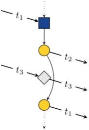
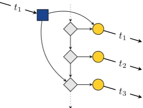
on the same station. These arcs make it possible for passengers to leave a train as it arrives at a station and transfer to any train that departs from that station at a later time. This construction is visualized in Figure 4.1.

t1

t2

t3

t1

Figure 4.1: Transfer construction at a station. Different vertex types (event types) are highlighted by shape: square (arrival), circle (departure) and diamond (crossing).

In Figure 4.1, all events are located at the same station and sorted in chronological order starting at the top of the figure. The arcs between the arrival events (squares) and departure events (circles) represent potential transfers. In this example traint1arrives first at the station. While it waits, a second traint2departs and

another traint3crosses the station without stopping. Passengers fromt1 can transfer tot2, stay int1 or

remain at the station. They are not able to transfer tot3, since this train does not stop at the station.

The model solves the single-source shortest path problem to find the all possible paths. Since the graph is directed and acyclic, this can be done in linear time using topological sorting. From all possible paths, the paths for the chosen departure times are extracted and connected to the departure groups, these are the nominal paths.

4.5 Realized paths

The nominal paths, as described in the previous section, give the paths and corresponding arrival times in case the timetable is executed exactly as planned. In a realization, the processes are subject to stochastic disturbances and hence, processes may take longer than expected. Trains may experience delay due to these disturbances or due to the delay of previous trains, in accordance with the definitions of primary and secondary delays from Section 1.5. To simulate the primary delays in the model, the process time of a processpis defined as the technically minimum process timel(p)plus a disruptionδ(p).

For a given disruption and corresponding primary delays, the secondary delays are included by a dy-namic program as displayed in the algorithm below (Mar´oti, 2017). An eventecan be realized as soon as all its predecessors in the graph representation allow it to happen. Additionally, departure events are not allowed to happen before their planned event time. The dynamic program calculates the realized event times, which are denoted byy(e).

foralle∗∈Edo

ife∗is a departure eventthen

y(e∗) := max{π˜(e∗); max{y(e) +l(p) +δ(p)|p= (e, e∗)∈P}};

else

y(e∗) := max{y(e) +l(p) +δ(p)|p= (e, e∗)∈P};

(25)

added to the graph between successive arrival and departure events on the same station. In the realization the chronological order of events can differ from the order the nominal graph, which results in different transfer possibilities.

In the calculation of passenger punctuality, NS assumes that passengers follow their planned route unless it requires rescheduling (van der Berg, 2015): It requires rescheduling if either a train departs with a delay larger than 15 minutes or when the planned route is no longer feasible because of, for example, a missed transfer. Therefore, the evaluation model uses the pessimistic principle regarding to the passengers’ route choice in the realized timetable. The constraint that routes are reconsidered if a train departs with a delay larger than 15 minutes is omitted, since the evaluation model is designed to simulate only small delays and because test runs show that the train delays never exceed the 15 minute threshold. Thus, the route is only rescheduled when the nominal path is no longer feasible.

Rescheduling methods

If it is not possible to follow the nominal path in the realization, an alternative must be chosen. In NS’ system, no dynamic rescheduling module is implemented. Instead of rescheduling the path of the passenger, the check-out time of the passenger is used to determine its arrival time at the check-out station, see Section 2.2.3. Unfortunately, the evaluation model cannot simulate the arrival times using the check-out data since such data is not available. The model has to reschedule the path using an alternative way. Due to the absence of a defined rescheduling procedure, various ways of rescheduling are considered below.

• Optimistic rescheduling: The easiest way is to determine an alternative for the whole path using the optimistic principle (Nielsen et al., 2009). Here, the shortest path that is found in the realization is chosen as alternative path. This is not the most realistic way, it suggests passengers can predict a missed transfer or delay and choose another path in advance. This method will likely result in an underestimation of the passenger delay (Nielsen et al., 2009).

• Realistic rescheduling: It would be more realistic to reschedule the path of a passenger from the point that the nominal path is no longer feasible in the realized graph, as suggested in the 3rdgeneration of passenger delay models (Nielsen et al., 2009). Therefore, the model follows the nominal path and finds the moment in time and station were a transfer is missed. From this station the shortest path in the realized graph is taken to the final destination to determine the final arrival time.

Both rescheduling methods are implemented into the evaluation model.

4.6 Output of the evaluation model

Once the paths, that are used in the realization, are determined, the delay of each path is calculated. The delay of a path is defined as the difference in arrival times of the nominal path and the used realized path. Given the reference timetable, ODT matrix, and the departure times of the departure groups, the model returns the average delay and punctuality. Besides the desired average passenger delay and passenger punctuality, the model also returns the average delay and train punctuality.

Train delay and punctuality

The average train delay is defined as the average delay of arrival events. The planned timesπ˜(e) and realized event timesy(e)of these events are compared and the difference is noted asDe, the delay of that

event. SoDe= max{0, y(e)−π˜(e)}. LetEarrdenote the subset of arrival events. The average train delay

¯

Dtrainis defined as

¯

Dtrain=

P

e∈EarrDe

|Earr|

.

The train punctuality is determined for a 5 and 15 minute threshold. In order to calculate the punctualities, the binary functionBis introduced.

B(De, x) = (

0 ifDe≥x,

(26)

The number of trains which arrive within the thresholds can be counted usingB. The train punctualities, denoted byPtrain,5andPtrain,15respectively, are defined by

Ptrain,5=

P

e∈EarrB(De,5)

|Earr|

and Ptrain,15=

P

e∈EarrB(De,15)

|Earr|

.

Passenger delay and punctuality

The evaluation model calculates the delays per passenger group, as discussed in Section 4.3.2. Let the set of departure groups be denoted byG. For every groupg ∈ Gthe arrival delayDg, whereDg ≥ 0, and

weight or group sizewgare stored. The average passenger delay is formulated as

¯

Dpassenger=

P

g∈Gwg·Dg P

g∈Gwg .

Here, the delay of a passenger group is weighted with corresponding number of passengers in that group. The sum of all weighted delays is divided by the total number of passengers. The punctualities, denoted by Ppassenger,5andPpassenger,15, are defined by

Ppassenger,5=

P

g∈Gwg·B(Dg,5) P

g∈Gwg

and Ppassenger,15=

P

g∈Gwg·B(Dg,15) P

g∈Gwg .

In these equations the functionB is used to determine whether or not each group delay lays within the specified threshold. The sum of the weighted outcomes ofBcorresponds with the total number of passen-gers who arrived within the threshold. Dividing this sum by the total number of passenpassen-gers results in the passenger punctuality.

4.7 Limitations and assumptions

The evaluation model is a simplified simulation of the execution of a timetable. As mentioned in Section 4.2, most of the input data is not available. Moreover, the journey planner in NS’ system is different from the shortest path design in the evaluation model, due to the transfer construction. In this section, all limitations and assumptions, that are made in the evaluation model, are discussed.

4.7.1 Input data

CICO data and frequent ODs

The number of passengers between each combination of stations is based on historic data; it is an estima-tion. Firstly the daily expected number of passengers is given by the OD matrix. The OD matrix, which is used in the evaluation model, is not the original classified matrix of NS but a modified version of it. This modification gives a rough idea of the expected number of passenger per day. The distribution of the pas-sengers over the hours of a day is also based on data from the past. The combination of the two estimations provides the CICO data for the evaluation model: the check in time, check in station, and the check out station. Moreover, the frequent ODs are determined: stations without any passengers are neglected.

Note that in both the OD matrix and the passenger distribution make no distinctions are made between different days of the week. The number of passenger and distribution during workdays is different from weekends and holidays.

Disturbances

It is complicated to determine the size or even the distribution of disturbances. All available realization data from the trains shows the total delay, this includes both primary and secondary delays. An analysis of the total delays to find a distribution is already complicated, but it is even more complicated to separate primary and secondary delays within the total delay, and to extract the disturbances.

(27)

The distribution in the evaluation model is equal to the distribution in SOM; which is an exponential distribution. Detailed analyses of realization data in the Netherlands showed that late arrivals, departures, and dwell time prolongations, all fit well into exponential distributions (Vromans, 2005). However, these results are based on a limited period of realization data and on one location only. Due to the lack of further knowledge about disturbances, exponentially distributed disturbances are used in both SOM and the evaluation model.

The means of the exponentially distributed disturbances are determined and a maximum is set using the default settings for SOM. In the default setting of the case study, which is analyzed in Chapter 5, the disturbances over movement processes are exponentially distributed with a mean of 5% of the technically minimal process time and a maximum of 5 minutes. The disturbances over the dwelling processes are exponentially distributed with a mean of 30% of the technically minimal process time with a maximum of 2 minutes. The question remains whether or not these choice of parameters will result in realistic delays, this question is out of scope for this thesis.

4.7.2 Journey planner

Passengers’ path choice

Another assumption in the evaluation model traces back to an assumption made in the calculation of the passenger punctuality, namely: the passenger wants to go as quickly as possible from A to B. Therefore, the model always chooses the shortest path, even if the passenger has a preference for another path (with less transfers for example).

Furthermore, NS has not defined a dynamic rescheduling method. Therefore, in this thesis, two res-cheduling methods as stated in Section 4.5.1 are proposed and implemented into the evaluation model.

Zero-minute transfers

Another remarkable feature of the evaluation model is transfer construction. The used construction allows passengers to make a transfer as long as the transfer time is nonnegative. Zero-minute transfers are pos-sible in the evaluation model. This simplifies the model but also makes some transfers pospos-sible that are impossible to make in real life.

An expansion of the zero-minute transfer structure is considered during the construction of the eval-uation model. The following construction, described by Bast et al. (2016) and M¨uller-Hannemann et al. (2007) as a realistic time-expanded model, makes transfers with minimal transfer times possible. Instead of direct arcs between the arrival and departure vertices, as is illustrated in Figure 4.2, additionaltransfer verticesare added to the graph for each departure event, see Figure 4.3. Note here that the minimum transfer time is different per station, per transfer and even per passenger.

t1

t2

[image:27.595.332.478.541.651.2]

t3

Figure 4.2: Current transfer construction at a station. Different vertex types (event types) are highlighted by shape: square (ar-rival) and circle (departure).

t1

t2

t3

Figure 4.3:Expanded transfer construction at a station. Different vertex types (event types) are highlighted by shape: square (arrival), circle (departure) and diamond (transfer vertex).

Both figures illustrate the same situation at a station. Traint1arrives at the station, followed by the departure

(28)

transfer to each of the three trains in the current model, see figure 4.2. The expanded transfer construction in Figure 4.3 makes it possible to add minimal transfer times to stations. Each arrival vertex is connected to the first transfer vertex that obeys the minimum change time constraints, that is the transfer node corresponding to the departure oft3in this example.

(29)

5 Computational results and data analysis

In this chapter, a timetable is evaluated using the evaluation model (see Chapter 4). The used timetable contains only a small part of the Dutch railway network due to the limitations of the evaluation model as we describe in Section 7.

The computational results are obtained by implementing the evaluation model in MATLAB R2016b running on Windows 10. The hardware was an Intel Core i7 processor with a clock speed of 2.4 GHz and 8 GB internal memory.

We consider an area around Utrecht and a timetable constructed in 2013. The area contains only two intercity stations; some large passenger flows that are not fully contained in the area are excluded. As a consequence, the area will experience relatively more transfers in relation to the whole Dutch railway system.

For this case study, the evaluation model creates days with a length of 12 hours. The mean size of the disturbances on the processes is determined by the default parameters of the timetable. The results in this chapter are obtained by running 1000 simulations of 12-hours days, each with independent stochastic disturbances. These simulations took over 40 hours of calculation time, running four simulations parallel at all times.

In Section 5.1, the results of the Utrecht case are presented. In Section 5.2, the data from the model is further analyzed. Moreover, the results of simulations with different disturbance vectors are presented in Section 5.3. Finally, the chapter is concluded in Section 5.4 with a summary.

5.1 Results Utrecht case

(30)

5.1.1 Train delay and punctuality

The delay of the trains is measured at each arrival event, each measured with the same weight. In Table 5.1 the average delay and average punctualities are given together with the corresponding 95% confidence intervals (CI). The confidence intervals are determined using the Batch Means Method (Alexopoulos et al., 1997). Additionally, a histogram of the distribution of the train delays is presented in Appendix B, see Figure B.1.

Table 5.1:Results of trains at arrival with default parameters.

Average 95% CI Train delay (minutes) 2.1092 [2.1050, 2.1133]

Train punctuality 5 minutes 89.14% [89.07%, 89.20%]

Train punctuality 15 minutes 100% [100%, 100%]

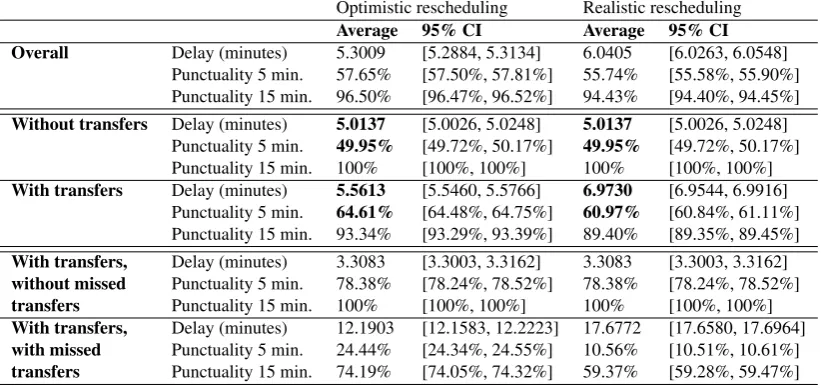
5.1.2 Passenger delay and punctuality

In the results of the passenger delay and punctuality, two variables are distinguished: the rescheduling method and the journey type. Two rescheduling methods are included into the evaluation model. The first method is denoted asoptimistic rescheduling, the complete journey is rescheduled using the realized timetable. The second way to reschedule is denoted asrealistic rescheduling, this method reschedules the journey of the passengers from the point they missed their transfer. Journeys are divided into several types and are assigned labels. We refer to the journey types using these labels throughout the remainder of this chapter. The labels’ descriptions are given below.

• Overallcontains, as the name suggests, all journeys.

• The journeys with a direct connection between their origin and destination station carry the label without transfers. Since they cannot miss a transfer, the results for the two methods of rescheduling will be identical.

• The remaining group of journeys, those who do have a transfer, are labeled:with transfer.

Within the group with transfers, a distinction is made between journeys which include a missed transfer, and those which do not.

• The group with transfers, without missed transfers were able to follow their promised path, the results of the two methods of rescheduling will again be identical.

• The groupwith transfers, with missed transfersdid miss a connection and had to reschedule their journey.

In Figure 5.1, the relative size of each journey type is displayed. The ratio between the number of journeys with and without transfers is independent of the simulations. However, the relative size of the number of journeys with missed transfers follow from the 1000 simulations. In the Utrecht case, the number of the journeys without transfers is slightly smaller than the group with transfers.

Evaluating and improving the passenger punctuality of a timetable

Master thesis - Applied Mathematics