Alternative prior distributions for variable selection with very many more variables than observations

University of Warwick institutional repository: http://go.warwick.ac.uk/wrap

This paper is made available online in accordance with

publisher policies. Please scroll down to view the document

itself. Please refer to the repository record for this item and our

policy information available from the repository home page for

further information.

To see the final version of this paper please visit the publisher’s website

.

Access to the published version may require a subscription.

Author(s): JE Griffin and PJ Brown

Article Title: Alternative Prior Distributions for Variable Selection with

very many more Variables than Observations

Year of publication: 2005

Link to published article:

http://www2.warwick.ac.uk/fac/sci/statistics/crism/research/2005/paper

05-10

Alternative prior distributions for variable selection

with very many more variables than observations

J.E. Griffin

Department of Statistics, University of Warwick, Coventry, CV4 7AL, U.K.

P.J. Brown

Institute of Mathematics, Statistics and Actuarial Science, University of Kent,

Canterbury, CT2 7NF, U.K.

15th May 2005

Abstract

The problem of variable selection in regression and the generalised linear model is ad-dressed. We adopt a Bayesian approach with priors for the regression coefficients that are scale mixtures of normal distributions and embody a high prior probability of proximity to zero. By seeking modal estimates we generalise the lasso. Properties of the priors and their resultant posteriors are explored in the context of the linear and generalised linear model es-pecially when there are more variables than observations. We develop EM algorithms that embrace the need to explore the multiple modes of the non log-concave posterior distribu-tions. Finally we apply the technique to microarray data using a probit model to find the genetic predictors of osteo- versus rheumatoid arthritis.

Keywords: Bayesian modal analysis, Variable selection in regression, Scale mixtures of

normals, Improper Jeffreys prior, lasso, Penalised likelihood, EM algorithm, Multiple modes, More variables than observations, Singular value decomposition, Latent variables, Probit regression.

1

Introduction

It is common nowadays to be able to investigate very many variables simultaneously with data collected on relatively few samples. For example in functional genomics microarray chips typically have as many as ten thousand genes spotted on their surface and their be-haviour may be investigated over perhaps one hundred or so samples. Curve fitting in pro-teomics and other application areas may involve an arbitrarily large number of variables, being limited only by the resolution of the instrument. In such circumstances often it is de-sirable to be able to restrict attention to the few most important variables by some form of adaptive variable selection.

Classical subset selection procedures are usually computationally too time consuming and perhaps more importantly suffer from inherent instability (Breiman, 1996). Bayesian stochastic search variable selection (SSVS) methods have become increasingly popular of-ten adopting the ‘spike and slab’ prior formulation of Mitchell and Beauchamp (1988), see also George and McCulloch (1997), Wolfe et al (2004), Brown et al (1998) for multivariate extensions and more recently in the more- variables- than- observations case by(k >> n), by Brown et al (2002), West (2003). In these approaches Bayesian averaging helps to induce stability. Despite careful use of algorithms to speed up computations these approaches are still too slow to deal with the vast numbers of variables (of order 10,000) of some applications and some form of pre-filtering is necessary.

One form of Bayesian approach which does offer the potential for much faster compu-tation takes a continuous form of prior and looks merely for modes of the posterior distri-bution rather than relying on MCMC to fully investigate the posterior distridistri-bution. Such formulations lead to penalised log likelihood approaches where the additive penalisation of the log likelihood is the log of the prior distribution. Tibshirani’s (1996) lasso is equiv-alent to a double exponential prior distribution, proposed in Bayesian wavelet analysis by Vidakovic (1998). A more extreme form of penalty is the normal-Jeffreys prior (Figueiredo and Jain 2001, Figueiredo 2003), adopted in an extended generalised linear model setting by Kiiveri (2003). From a different viewpoint Fan and Li (2001) have modified the lasso’sL1

penalty so as to offer less shrinkage for large effects, see also Fan and Peng (2004).

Early examples of parallel approaches in the machine learning literature are Automatic Relevance Determination of Mackay (1994) and the Relevance Vector Machine of Tipping and Faul (2003).

in-formation. In the probit case, our method of hyperparameter choice is geared to prediction characteristics of some canonical models and although data dependent helps to avoid over-shrinkage. We finish by analysing microarray data on two forms of arthritis earlier analysed by Sha et al (2003).We embrace the multimodality through plots of genes included in modes as ranked either by posterior or log-likelihood value. We are able to reveal subsets of highly discriminating genes.

2

Generalising lasso estimation

There are at least two ways of generalising the lasso in a Bayesian setting. One is to use an exponential power prior forβ, see Box and Tiao (1973, p157); the other is to use a scale mixture of normals, see West (1987). Non Bayesian analogues and adaptations of the former are to be found in Knight and Fu (2000), Fan and Li (2001). We will rather devote our attention to scale mixtures of normals as these are easier to deal with analytically and are richer in form.

2.1

Scale mixture of normal prior distributions

If we wish to construct distributions that bridge the gap between the normal-Jeffreys prior and the double exponential distribution, a natural class of prior distributions to consider for each regression coefficient,βi, would be scale mixtures of normal distributions where

π(βi) =

Z

N(βi|0, ψi)G(dψi) (1)

where N(Y_|µ, σ2_{)denotes the probability density function of a random variableY having a}

normal distribution with meanµand varianceσ2.HereGis the mixing distribution and its density, if it is defined, will be referred to asg(_·). The prior variance of the regression coef-ficients, if it exists, can be simply expressed in terms of the mean of the mixing distribution since

V(βi) =Eψi(V(βi|ψi)) +Vψi(E(βi|ψi))

=Eψi(V(βi|ψi))

=Eψi(ψi).

If we assume that domain knowledge will not be included in the prior, the mixing distribution seems a natural place to include the belief that only a few regressors will be important to give a good fit to the data. Most Bayesian approaches to variable selection make use of the form

1988, George and McCulloch, 1997), expresses the prior distribution for βi as a mixture

distribution

i_.e_{. π(βi) =θN(βi|0, σ}2

β) + (1−θ)δβi=0 (2)

where δx=a is the Dirac measure which places measure 1 on {x = a}. The parameter

0 < θ <1can be interpreted as the probability that a variable is included in the model and

σ_β2 is the prior variance of the regression coefficients included in the model. If we make use of the obvious extension of the normal distribution by defining N(x_|µ,0) = δxi=µ, the

mixing distribution can be expressed as

g(ψi) =θ δψi=σβ2 + (1−θ)δψi=0. (3)

Other particular mixture distributions of interest can also be represented in this scale mixture form.

1. The mean-zero double exponential distribution, DE(0,1/γ) with probability density function

1

2γ exp{−|β|/γ}, −∞< β <∞, 0< γ <∞

is defined by an exponential mixing distribution, Ex

1 2γ2

, with probability density function

g(ψi) =

1 2γ2exp

−ψi/[2γ2] . (4)

2. The normal-Jeffreys (NJ) prior distribution arise from the improper hyperprior

g(ψi)∝

1

ψi

, (5)

which in turn induces an improper prior forβiof the formπ(βi)∝ _|β1_i|.

3. A well-known result shows that the Studenttdistribution onλ >0degrees of freedom, scale parameterγ >0,can be expressed using an inverse-gamma mixing distribution

g(ψi) =IG

λ

2,

γ2λ

2

, (6)

where IG(a, b)is the inverse of a gamma with shapeaand natural parameterb.

4. One possible extension to the exponential mixing distribution is the gamma distribution

g(ψi) =Ga

ψi

λ, 1

2γ2

distribution of β is often called a normal-gamma (NG) or variance-gamma distribu-tion which has proved a popular choice for modelling fat tails in finance (e.g. Bibby and Sorensen, 2003) and is a member of the generalized hyperbolic family (see e.g. Barndorff-Nielsen and Blaesild 1981). The marginal distribution ofβihas the density

π(βi) =

1

√

π2λ−1/2_γλ+1/2_Γ(λ)|βi|

λ−1/2_K

λ−1/2(|βi|/γ) (8)

whereKis the modified Bessel function of the third kind. The variance ofβi is2λγ2

and the excess kurtosis is 3_λ.

5. Another extension arises from placing a further mixing distribution on the scale pa-rameter of the exponential mixing distribution. A gamma mixing distribution with parameters λ, γ2 on the natural parameter of the exponential leads to a subclass of the gamma-gamma distribution (Bernardo and Smith, 1994, p120). The density of the mixing distribution onψi has the form

g(ψi) =

λ

γ2(1 +ψi/γ

2₎−(λ+1) _{0< λ, γ <∞. (9)}

The density of the marginal distribution ofβi can be expressed as

π(βi) =

λ √

π

2λ

γ Γ(λ+ 1/2) exp

1 4

β2

γ2

D_−2(λ+1/2)

|β_| γ

(10)

whereDν(z) is the parabolic cylinder function. Computation of this functions is

de-scribed in Zhang and Jin (1996, section 13.5.1, p439), coded versions are available

fromhttp://jin.ece.uiuc.edu/routines/routines.htmlfor Fortran

77 andhttp://ceta.mit.edu/comp_spec_func/for Matlab. Ifλis small, the computation of exp_{z_}Dν(z) is much more stable than computation of Dν(z).

This involves a simple modification of the method described in Zhang and Jin (1996). The parameter γ and λ control the scale and the heaviness of the tails respectively. From Abramowitz and Stegun (1964, p689 eqn 19.8.1) we see that for large |βi|

γ

π(βi)≈c

|βi|

γ

−(2λ+1)

.

Also if λ > 1, the expectation of ψi and the variance ofβi exist and have the form γ2

(λ−1). The excess kurtosis is3λ−λ2 ifλ > 2. This class of distributions, unlike the

normal-gamma class, can define distributions for which the variance is undefined and thus has a rather different tail-to-spike balance. The distribution function ofψi is also

available in closed form as

G(ψi) = 1−

1 + ψi

γ2

−λ

We will refer to the marginal distribution ofβiwith density (10) as the

normal-exponential-gamma (NEG) distribution and the marginal distribution of ψi as the

exponential-gamma (EG) distribution.

We would expect all of these methods to improve upon a normal prior distribution with fixed variance, which would have the mixing distribution

g(ψi) =δψi=σβ2,

since moving some mass in the mixing distribution either to zero in the case of (3) or close to zero in (4), (5), (6), (7) and (9) is consistent with our prior belief that many of the regression coefficient are close to zero and hence their values will be drawn from distributions with small variances. A natural starting point would be to re-consider equation (4) and question whether it accurately reflects our prior beliefs. If not, a wider class of prior distribution can be generated by elaborating the exponential mixing distribution, leading to the Studentt,NG or NEG above. The relative merits of these are discussed in what follows.

2.2

Shapes and Limits

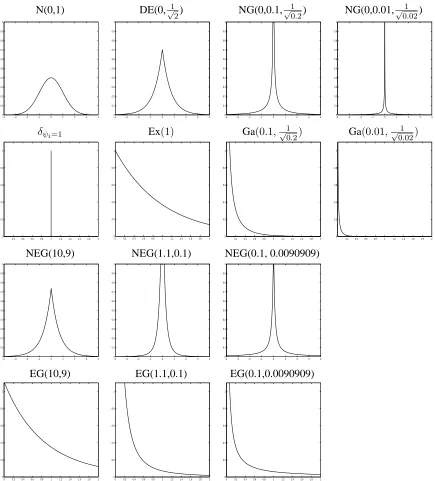
Some of the mixing distributions described above and their corresponding densities forβare displayed in Figure 1. Generally the expectation of the normal varianceψis fixed at unity by appropriate setting of the hyperparameters, except when this does not exist as in the last pair of figures when for the NEGλ= 0.1, for which the expectation of1/ψis fixed at unity.

Aside from incorporating the density of the ‘lasso’ as a special case many of the scale mixture of normals will have the normal-Jeffreys as a limiting density form. For example the normal-gamma (NG) given by (8) goes to this improper limit whenλ _↓ 0 andγ _{↑ ∞}. This degenerate limiting form has infinite mass, an infinite spike at zero and flatness for large values of_|β_|,and as a consequence does not penalise such large values. The spike at zero has strong consequences for the modal behaviour of the posterior, not all of them welcome as we shall see. Whereas the normal-gamma does have an infinite spike at zero forλ_≤1/2, the normal-exponential-gamma distribution has the advantage of a finite limit at zero for all parameters values in its range and incorporates as limiting cases the double exponential prior (asλ, γ _{↑ ∞}) and the normal-Jeffreys case (asλ, γ _↓ 0).

N(0,1) DE(0,√1

2) NG(0,0.1,

1 √

0.2) NG(0,0.01, 1 √

0.02)

−4 −3 −2 −1 0 1 2 3 4 0 0.1 0.2 0.3 0.4 0.5 0.6 0.7 0.8 0.9 1

−4 −3 −2 −1 0 1 2 3 4 0 0.1 0.2 0.3 0.4 0.5 0.6 0.7 0.8 0.9 1

−4 −3 −2 −1 0 1 2 3 4 0 0.1 0.2 0.3 0.4 0.5 0.6 0.7 0.8 0.9 1

−4 −3 −2 −1 0 1 2 3 4 0 0.1 0.2 0.3 0.4 0.5 0.6 0.7 0.8 0.9 1

δψi=1 Ex(1) Ga(0.1,

1 √

0.2) Ga(0.01,

1 √

0.02)

0.2 0.4 0.6 0.8 1 1.2 1.4 1.6 1.8 2 0 0.2 0.4 0.6 0.8 1

0 0.2 0.4 0.6 0.8 1 1.2 1.4 1.6 1.8 2 0 0.2 0.4 0.6 0.8 1

0.2 0.4 0.6 0.8 1 1.2 1.4 1.6 1.8 2 0 0.2 0.4 0.6 0.8 1

0.2 0.4 0.6 0.8 1 1.2 1.4 1.6 1.8 2 0 0.2 0.4 0.6 0.8 1

NEG(10,9) NEG(1.1,0.1) NEG(0.1, 0.0090909)

−4 −3 −2 −1 0 1 2 3 4 0 0.1 0.2 0.3 0.4 0.5 0.6 0.7 0.8 0.9 1

−4 −3 −2 −1 0 1 2 3 4 0 0.1 0.2 0.3 0.4 0.5 0.6 0.7 0.8 0.9 1

−4 −3 −2 −1 0 1 2 3 4 0 0.1 0.2 0.3 0.4 0.5 0.6 0.7 0.8 0.9 1

EG(10,9) EG(1.1,0.1) EG(0.1,0.0090909)

0 0.2 0.4 0.6 0.8 1 1.2 1.4 1.6 1.8 2 0 0.2 0.4 0.6 0.8 1

0 0.2 0.4 0.6 0.8 1 1.2 1.4 1.6 1.8 2 0 0.2 0.4 0.6 0.8 1

0 0.2 0.4 0.6 0.8 1 1.2 1.4 1.6 1.8 2 0 0.2 0.4 0.6 0.8 1

Figure 1: Various forms considered for the prior distribution forβ with their associated mixing distribu-tion

−1 −0.8 −0.6 −0.4 −0.2 0 0.2 0.4 0.6 0.8 1 −70

−60 −50 −40 −30 −20 −10 0 10 20

−1 −0.8 −0.6 −0.4 −0.2 0 0.2 0.4 0.6 0.8 1 −70

−60 −50 −40 −30 −20 −10 0 10 20

(a) (b)

−1 −0.8 −0.6 −0.4 −0.2 0 0.2 0.4 0.6 0.8 1 −70

−60 −50 −40 −30 −20 −10 0 10 20

−1 −0.8 −0.6 −0.4 −0.2 0 0.2 0.4 0.6 0.8 1 −70

−60 −50 −40 −30 −20 −10 0 10 20

(c) (d)

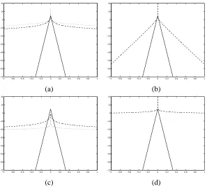
Figure 2: Log prior densities setting the central region (-0.01,0.01) to have probability η = 0.9for: (a) double exponential distribution (solid line), NEG (λ= 1) (dashed line) and NEG(λ= 0.1) (dotted line), (b) double exponential distribution (solid line) and NG (λ = 0.1) (dashed line), (c) double exponential (solid line),t-distribution (λ = 2) (dashed line) andt-distribution (λ= 0.2), and (d) double exponential (solid line) and improper normal-Jeffreys (dashed line)

without the drawback of the extreme spike at zero.

2.3

Thresholding for variable selection

The five distributions can express our belief that a small number of regressors can fit the data well but also allow a wide-range of other properties. It is important to choose appropriate forms that lead to a useful variable selection procedure.

A standard interpretation of Bayes theorem, is that the log posterior distribution is addi-tive in data and prior information as given by

logπ(β_|y) = logf(y_|β) + logπ(β), (11) where log probability is a measure of utility (Bernardo and Smith, 1994). It is natural to regard the negative prior utility as a penalty function given asp(β),where

It is the relative contribution of the two components on the right hand side of (11) that de-termines the posterior. Turning points of the posterior are then obtained by setting to zero the derivative of (11) and hence depend on the sum of the classical efficient score function,

−∂logf(y_|β)/∂β and the derivative of the penalty function. In the case of a single pa-rameter, we will generally assume that turning-point (TP) thresholding, that is setting the penalized estimatorβ˜ = 0, will occur iff there is no turning point. In which case with the class of penalty functions considered, the posterior is monotone decreasing in_|β_|that is the only mode is atβ = 0. Strictly if there is a turning point and the posterior function is non monotone then there may also be a mode at zero. A preference for a turning point follows the approach of Fan and Li (2001) and could be more formally computed by consideration of probability mass in the neighbourhood of zero, even when there is a spike at zero. An alternative choice, more simply computed with many regressors, is the true posterior mode which will be called the Bayesian threshold, that is the mode with the highest posterior mass. If there is one regressor, the lasso case, where the prior distribution is double exponential, is the only one of our chosen distributions where these thresholds are identical (see Appendix 1). Various penalty functions together with their derivatives are listed in Table 1.

p(β) p0_(|β|)

double exponential(0,_γ1) |β_γ| 1_γ

normal-Jeffreys log_|β_{| |β}1_|

IG

λ

2

λγ2

2

λ+1

2 log(1 +β2/λγ2) λγλ2+1_+β2|β| normal-gamma 1_{2 −}λ

log_|β_{| −}logK_λ−1/2|β_γ| 1_γKλ−3/2

|β|

γ

Kλ−1/2 |βγ| NEG ₋₄β_γ22 −logD_−2(λ+1

2)

|β|

γ

(λ+1/2)

γ

D−2(λ+1) |β_γ|

D_{−2(λ+ 1}

2 )

|β|

γ

Table 1:Penalty functions and their derivatives induced by various choice for the hyperprior

Our approach will be applied to the generic problem of multiple regression, with the generalised linear model as a possible extension. It is assumed that we observe an(n_× k) -dimensional data matrix, X, and an (n_× 1)-dimensional response, y. The relationship between the responses and the data is modelled by a linear regression

π(y_|β, σ2, X) =N(y_|Xβ, σ2I)

where N(x_|µ,Σ) denotes a multivariate normal distribution with mean µ and variance Σ. The problem of finding a maximum a posteriori (MAP) estimate ofβ can be expressed as a penalised likelihood problem whereβis chosen to find a minimum of the function

L= 1

2σ2(y−Xβ)

T_(y

−Xβ) +

k

X

i=1

0 0.1 0.2 0.3 0.4 0.5 0.6 0.7 0.8 0.9 1 0

1 2 3 4 5 6 7 8 9 10

0 0.1 0.2 0.3 0.4 0.5 0.6 0.7 0.8 0.9 1 0

1 2 3 4 5 6 7 8 9 10

(a) (b)

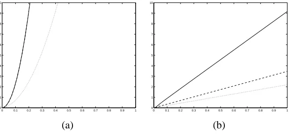
Figure 3: TP thresholding rule forβˆas a function of the standard error under different prior choices with

η = 0.9 and = 0.01: (a) double exponential distribution (solid line) and normal-gamma (λ = 0.1) (dotted line), and (b) normal-exponential-gamma distributions withλ = 10(solid line), λ = 1(dashed line) andλ= 0.1(dotted line)

wherep(x) =₋logπ(x)is the penalty function. In generalised linear models the negative log-likelihood or deviance replaces the first term of (12). A particular case is probit regression as applied in section 4 where the information content of the likelihood is somewhat less than in the normal linear model.

Fan and Li (2001) consider the link between the choice of penalty function (or prior dis-tribution in our case) and the TP thresholding value. The MAP estimate will be zero only if the maximum likelihood estimate (MLE) is smaller than this threshold value. In a uni-variate regression problem, for the maximum likelihood estimatorβˆ, the parameter is set to zero if_|βˆ_|<minθ6=0{|θ|+ σ

2

XT_Xp0(|θ|)}wherep0(·)is the derivative of the penalty function

and √ σ

XT_X is the standard error of βˆ. A comparison with some of the prior distributions

described above is illuminating. For the double exponential prior distribution, thresholding occurs if_|βˆ_| < _γ1_XσT2_X which depends on the square of the standard error. In contrast, the

normal-Jeffreys prior thresholds according to the rule_|βˆ_| < 2√ σ

XT_X and the thresholding

depends linearly on the standard error. Figure 3 compares the thresholding rules for the normal-gamma penalty and the normal-exponential-gamma penalty. The latter has linear be-haviour where the slope depends onλ, generalising the normal-Jeffreys rule and is thus more appealing. The normal-gamma case has substantially different behaviour and defines a much more conservative criterion. Much larger values ofγ would induce a linear thresholding rule but this contradicts our imposed prior property of a large mass close to zero.

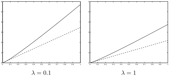
The Bayesian threshold for the normal-Jeffreys and normal-gamma choices with λ <

0 0.1 0.2 0.3 0.4 0.5 0.6 0.7 0.8 0.9 1 0

1 2 3 4 5 6

0 0.1 0.2 0.3 0.4 0.5 0.6 0.7 0.8 0.9 1 0

1 2 3 4 5 6

λ= 0.1 λ= 1

Figure 4: Bayesian threshold (solid line) and TP threshold (dashed line) for the NEG prior distribution withη= 0.9and= 0.01

Bayesian threshold is more conservative and almost doubles the thresholding value.

The discussion so far has centred around thresholding but the choice of penalty function will also have implications for the shrinkage of non-zero estimates. For example, Johnstone and Silverman (2005) suggest that overshrinkage of non-zero estimates can lead to better predictive performance in wavelet regression. Differentiating (12), the relationship between the penalised MLEβ˜and the MLEβˆ

ˆ

β₋β˜ σ2_/Pn

i=1x2i

=sign( ˜β)p0(_|β˜_|)

shows that the amount of shrinkage is directly controlled by the derivative of the penalty function. Figure 5 illustrates various choice of penalty function with a chosen value of the probability massηon the interval(₋, ). The flat tails of the Jeffreys and normal-exponential-gamma distributions lead to small derivative for large values ofβˆand β˜ _≈ βˆ, which implies the so-called oracle property of Fan and Li (2001). The normal-gamma choice maintains a substantial derivative in the tails (which is approximately1_γ).

2.4

Modal estimates with multiple parameters

The following section extends the univariate results to problems with two regressors. First, for k parameters, returning to the penalised likelihood function, L, the derivative can be expressed as

dL

dβ = X

T_Xβ−XT_y+sign(β)p0_(|β|)

(XTX)−1dL

dβ = β−βˆ+ (X

−1 −0.8 −0.6 −0.4 −0.2 0 0.2 0.4 0.6 0.8 1 0

50 100 150 200 250 300 350 400 450 500

−1 −0.8 −0.6 −0.4 −0.2 0 0.2 0.4 0.6 0.8 1 0

50 100 150 200 250 300 350 400 450 500

−1 −0.8 −0.6 −0.4 −0.2 0 0.2 0.4 0.6 0.8 1 0

50 100 150 200 250 300 350 400 450 500

(a) (b) (c)

Figure 5: Penalty functions ifη = 0.9and= 0.01for: (a) double exponential distribution (solid line), NEG (λ = 1) and NEG(λ = 0.1), (b) double exponential distribution (solid line) and NG (λ = 0.1) (dashed line), and (c) double exponential (solid line) and normal-Jeffreys (dashed line)

where

sign(β) = 

  

sign(β1) 0

. ..

0 sign(β2)



  

,_|β_|= 

  

|β1|

.. .

|β2|



  

Turning points away from zero can only occur if there exists a value of β for which some elements of dL_dβ are zero. The mode with the largest number of non-zero parameter estimates will be preferred. In the bivariate case, we assume that

XTX = c −ρ

√ cd −ρ√cd d

!

wherecanddare the sum of squares for the first and second variable respectively andρis the correlation between the maximum likelihood estimatorsβˆ1 andβˆ2, which has the opposite

sign to the correlation between the two independent variables

2.4.1 Lasso Regions

The relationship between thresholding and the values ofβˆ1andβˆ2can be studied analytically

for the lasso penalty. There are five regions into whichβˆ1andβˆ2can fall which are shown in

figure 6 (only positive correlation is considered; the relationship betweenβˆ1and−βˆ2shows

the effect of negative correlation) and derived in the Appendix 2. Four of these regions arise when there is a single posterior mode. Each region is defined by a combination of thresholding or not thresholding either estimate. However, a bimodal posterior distribution is also possible and figure 6 shows the values ofβˆ1and βˆ2 which lead to it as the lighest of

ρ= 0.5 ρ= 0.8 ρ= 0.99

lasso

−3 −2 −1 0 1 2 3 −3

−2 −1 0 1 2 3

−3 −2 −1 0 1 2 3 −3

−2 −1 0 1 2 3

−3 −2 −1 0 1 2 3 −3

−2 −1 0 1 2 3

normal-gamma

λ= 0.4

normal-Jeffreys

NEG

λ= 0.1

−3 −2 −1 0 1 2 3 −3

−2 −1 0 1 2 3

−3 −2 −1 0 1 2 3 −3

−2 −1 0 1 2 3

−3 −2 −1 0 1 2 3 −3

−2 −1 0 1 2 3

NEG

λ= 1

−3 −2 −1 0 1 2 3 −3

−2 −1 0 1 2 3

−3 −2 −1 0 1 2 3 −3

−2 −1 0 1 2 3

−3 −2 −1 0 1 2 3 −3

−2 −1 0 1 2 3

Figure 6: The regions where different types of thresholding occur either moving through shades of grey from black to white: only mode at 0 (black); β1 set to zero only; β2 set to zero only; two local modes;

internal mode (white) forc= 1,b= 1

ˆ

β1 and βˆ2 where no thresholding occurs clearly define four disjoint squares. This property

is independent of correlation but the region where both regressors are thresholded forms a rhomboid whose shape changes with the value ofρ. This agrees with the observation that if there is high correlation between the regressors there is a tendency for the MLEs to produce spurious relationships. In those situations, βˆ1 and βˆ2 have similar absolute values and the

predicted values will be near constant. The volume of the region will be determined by the ratios _γ√1

c and

1

γ√d.

2.4.2 General Regions

In contrast with the lasso regions, the shapes of non-thresholded regions (white in figure) depend on the correlation for the normal-gamma and normal-Jeffreys penalty functions (Fig-ure 6). These relationships are less amenable to analytical work and the regions are drawn by finding the type of thresholding on a grid of values. Both penalty functions lead to similar regions which are substantially different to those defined by the lasso penalty. Two striking differences are the shape of the region where both variables are thresholded and the shape of the region with a bimodal posterior. If both ML estimators have the same sign the no thresh-olding region becomes larger whereas if the signs are different the no threshthresh-olding region becomes smaller. The gap is filled by an expansion of the region with a bimodal posterior. These regions are intermediate between full thresholding (black) and no thresholding (white). This region is small and close to all axes with the double exponential prior but the shape de-pends on the correlation in the NEG case. In fact, the largest value of the correlation leads to this region filling almost all of the two quadrants whereβˆ1 and βˆ2 have opposing signs.

In other words, the thresholding depends on the difference ofβˆ1andβˆ2 and for correlations

close to₋1,the thresholding depends on the sum ofβˆ1andβˆ2.

The lasso and NEG penalties also define Bayesian thresholding regions (Figure 7). Un-like the one-dimensional case, the Bayesian and TP thresholding regions differ with a lasso penalty. The bi-modal region is divided into regions where one variable is thresholded. In contrast, the NEG penalty defines a substantially larger region where both estimates are shrunk to zero. Otherwise one of the regressors is set to zero and the lineβˆ1 =−βˆ2acts as a

dividing line between these two cases. The difference in thresholding between the lasso and NEG penalty suggest that the latter will shrink more variables from the model.

It is hard to make any general comments about thresholding in higher dimensions, suffice that there aremin(n, k)non-zero estimates. In the case of infinite spikes at zero (NJ, NG for

ρ 0.5 0.8 0.99

lasso

−3 −2 −1 0 1 2 3 −3 −2 −1 0 1 2 3

−3 −2 −1 0 1 2 3 −3 −2 −1 0 1 2 3 NEG

λ= 0.1

−3 −2 −1 0 1 2 3 −3 −2 −1 0 1 2 3

−3 −2 −1 0 1 2 3 −3 −2 −1 0 1 2 3

−3 −2 −1 0 1 2 3 −3 −2 −1 0 1 2 3 NEG

λ= 1

−3 −2 −1 0 1 2 3 −3 −2 −1 0 1 2 3

−3 −2 −1 0 1 2 3 −3 −2 −1 0 1 2 3

−3 −2 −1 0 1 2 3 −3 −2 −1 0 1 2 3

Figure 7: The Bayesian thresholding region with a NEG distribution. The parameters are chosen such thatπ(β _∈[₋0.01,0.01]) = 0.25for various values ofλ.

2.5

Relationship to model choice

Heuristically, we can think of the posterior mode as a variable selection method since setting a regression coefficient to zero removes a variable from the model. It is useful to define an indicator variable si that takes the value 0 if thei-th regressor is excluded from the model

(whenβˆi = 0) and 0 otherwise (whenβˆi = 06 ). For fixeds= (s1, . . . , sk), local posterior

modes obey the condition

0 =β?₋βˆ?_{+ (X}?T_X?₎−1_sign(β?_)p0_(|β?

|)

whereX? _{is the submatrix ofXconstructed using the columns for whichs}

i = 1andβ? =

{βi|si= 1}. If such a posterior modeβ˜? exists then

ˆ

β? _{= ˜β}?_{+ (X}?T_X?₎−1_{sign( ˜β}?_)p0_(|β˜?_|)

whereβˆ?_{is the ML estimate ofβ}?_{. The value ofsthat minimises}

L= 1

2σ2(y−X

?_β˜?₎T_(y

−X?β˜?_{) +} X

i|si=1

p(_|β˜_i?_|) + X

i|si=0

corresponds to the global posterior mode ofβ. The normal-Jeffreys and NEG with smallλ

define a penalty that is almost constant for a range of suitably large values ofβ˜?

i. This penalty

is represented byp1andLsimplifies to

L= 1

2σ2(y−X

?_β˜?₎T_(y−X?_β˜?_{) +rp}

1+ (k−r)p2

= 1

2σ2(y−X

?_β˜?₎T_(y−X?_β˜?_{) +k p}

2+r(p1−p2)

wherep2 =p(0)andris the number of non-zero estimates. The termk p2is constant across

allsand can be dropped which leaves the criterion

1

σ2(y−X

?_β˜?₎T_(y−X?_β˜?_{) + 2r(p}

1−p2),

where the first term is more generally the deviance.

The indicator variables that correspond to the posterior mode defines a model selection criterion that is a trade-off between goodness-of-fit and a penalty for each included parameter. This form has been a recurring idea in the model selection literature. Standard choices for the penalty are Akaike’s information criteria (AIC) (Akaike, 1974) wherep1−p2 =−1and

a Bayesian variant (BIC) (Schwarz, 1978)p1 −p2 = −1₂logn. A typical choice for NEG

ofλ = 0.1, η = 0.9and = 0.01 would lead to values of p1 −p2 around -15, which is

substantial larger than the penalties under the AIC and BIC for values ofnwhich are of the order of hundreds of observations. The penalty is much closer to the Risk Inflation Criterion (RIC) (Foster and George 1994) who choosep1−p2=−logkfor largek.

A further decomposition shows the relationship between the residual sum of squares calculated using the least squares estimates,

1

σ2(y−X

?_βˆ?₎T_(y

−X?βˆ?_{) +} 1

σ2(p0(|β˜?|))

T_(X?T_X?₎−1_p0_(|β˜?_{|) + 2r(p}

1−p2).

3

Inference for regression and probit regression

This section discusses posterior inference, in particular methods for finding local posterior modes, for probit regression models using the classes of prior distributions already described. Initially we concentrate on estimation for a normal prior distribution which will be an impor-tant component of our analysis.

3.1

Estimation with normal prior distributions

The prior distribution forβ,(k_×1)is assumed to have the form

whereΨis a (k_×k)-matrix. Typically this matrix will be a diagonal matrix although the derivations in this section do not assume this special form. The standard MLE estimator will not be defined ifkis larger thann. Consequently, the problem is re-expressed in terms of an

n-dimensional parameter,γ, for which the MLE exists. As in West (2003), the singular value decomposition ofXcan be written asX =FTDAT whereAis(k_×n)-dimension matrix such thatATA=In,Dis an(n×n)-dimension diagonal matrix andFis(n×n)-dimension

matrix for whichFT_{F =I}

nandF FT =In. Clearly, we can write

Xβ= (FTD)γ

whereγ =ATβ and the MLE,γˆ, ofγ is well-defined and has the form

ˆ

γ =D−1F y.

The sampling distribution γˆ and the prior distribution of the n-dimensional parameter γ

which is estimated byγˆcan be represented as

π(ˆγ_|γ,Ψ, X) =N(ˆγ_|γ, σ2D−2 = Λ?), π(γ_|Ψ, X) =N(0, ATΨA= Ψ0)

and the posterior distribution ofγis

π(γ_|ˆγ,Ψ, X) =N(γ_|Ψ0(Ψ0+ Λ?)−1ˆγ,(Λ?−1+ Ψ0−1)−1). (14)

In order to calculate the posterior distribution of the regression parameters,β, we consider the full singular value decomposition which represents X asFTD∗KT where the first n columns ofK,(k_×k)areA,(k_×n),the last(n₋k)columns asCgiven asK= (A , C),

andD∗,(n_×k)with

D?= D 0

.

In this case,KTK=IkandKKT =IkandKis invertible withK−1=KT. Ifγ? =KTβ,

the first nelements of γ? _{are γ and we define the last (k−n) elements to be τ. In this}

parametrizationτare exactly those dimensions that are independent of the data. Using this re-parametrization, the posterior distribution ofβ is simply related to the posterior distribution forγ?_{which can be expressed as}

π(γ?_|γ,ˆ Ψ, X) =π(τ_|γ,Ψ)π(γ_|γ,ˆ Ψ, X)

where

E(γ_|γ,ˆ Ψ) = Ψ0(Ψ0+ Λ?)−1ˆγ

and

E(τ_|γ,ˆ Ψ) =CTΨA(ATΨA)−1E(γ_|γˆ).

The normality of bothπ(τ_|γ,Ψ)andπ(γ_|γ,ˆ Ψ, X)combined with the linear mean ofτ inγ

implies thatγ?_{has a normal posterior distribution. The transformation fromβis well-defined}

and has the formβ =Kγ? implying thatβ will also be normally distribution a posteriori. This distribution can be characterised by its posterior mean and variance. Computationally, we want to calculate these quantities whilst avoiding inversions of(k_×k)-dimensional ma-trices. After some simplification we can express the posterior mean and covariance in a form where only matrix that needs inverting is ann_×n-dimension matrix

E(β_|Ψ,γˆ) = ΨA(ATΨA)−1E(γ_|ˆγ,Ψ)

= ΨA(ATΨA)−1(Ψ₀−1+ Λ?−1)−1Λ?−1ˆγ

= ΨA(Ψ0+ Λ?)−1ˆγ (15)

and

V(β_|Ψ,ˆγ) = Ψ₋ΨA(ATΨA)−1ATΨ + ΨA(ATΨA)−1Vγ|γ,ˆΨ(γ)(ATΨA)−1ATΨ

= Ψ₋ΨA(ATΨA)−1ATΨ + ΨA(ATΨA)−1(Ψ−₀1+ Λ?−1)−1(ATΨA)−1ATΨ

= Ψ₋ΨA(Ψ0+ Λ?)−1ATΨ. (16)

Finally, we note that the marginal distribution ofγˆgivenΨcan also be derived and has the form

π(ˆγ_|Ψ) =N(0, ATΨA+σ2D−2). (17)

3.2

Bayesian binary regression

The analysis of binary data arising from microarray experiments can exploit the normal the-ory developed thus far by introducing latent variables. There is also appeal in working di-rectly with the log-likelihood as discussed earlier, see Kiiveri (2003). However here we focus on the method proposed by Albert and Chib (1993) which exploits a latent variable charac-terisation to reduce probit regression analysis to that of regression albeit at the expense of creating nlatent variables. We assume that the response for the i-th individual is zi and

introduces latent parametersyisuch that

andyi>0 ⇐⇒ zi = 1. The model forziis a traditional probit regression analysis

π(zi= 1|β) = Φ(Xiβ).

whereΦ is the cumulative distribution function of a standard normal distribution. Impor-tantly, ifβ has a normal prior distribution, the posterior distribution of β_|y1, . . . , ynis also

normal.

Much of the work using normal-Jeffreys penalty functions, Kiiveri (2003), Figueiredo (2003)) attempts to find a single mode. Bae and Mallick (2004) and Mallick et al (2005) on the other hand go for full posterior simulation using MCMC, but in favouring the NJ overlooks the fact that the likelihood times prior for this remains improper as the likelihood forβat zero is bounded away from zero and hence the behaviour in the region of zero is still proportional to1/β and integrates to log(β),which blows up at zero.See Gelfand and Sahu (1999) for more detailed analysis of such improprieties. This precludes full Bayesian posterior anal-ysis using the NJ prior but does formally allow it to act as a device for generating modes from the ‘likelihood times prior’ in the spirit of penalised likelihood. It is yet another reason for our preference for the NEG which retains some of the attractions of NJ but without the dominating spike at zero.

3.3

Choosing hyperparameters

The standard subjectivist interpretation of the prior distribution is an expression of our beliefs about the likely values ofβand, in this case, the number of non-zero regression coefficients needed to explain the variation in the responses. However, this approach can be problematic when combined with the MAP estimation procedure. Consider a probit regression model with a relatively diffuse prior distribution forβ0 (in the sense that its effect can be ignored

when comparing local modes). The penalized likelihood function is

L=

n

X

i=1

zilog Φ(β0+Xiβ) + n

X

i=1

(1₋zi) log(1−Φ(β0+Xiβ))− k

X

i=1

p(_|βi|).

If only thej-th regressor takes a non-zero value,β˜j, and the intercept isβ˜0(j)then

L=

n

X

i=1

zilog Φ( ˜β0(j)+Xijβ˜j)+ n

X

i=1

(1₋zi) log(1−Φ( ˜β0(j)+Xijβ˜j))−p(|β˜j|)−(k−1)p(0).

Comparing this value to the penalized log likelihood for a “null model” for which all regres-sion coefficients, except the intercept, are set to zero shows that the “null model” will be superior unless there is at least one regressor for which

n

X

i=1

zilog

Φ( ˜β₀(j)+Xijβ˜j)

Φ( ˜β0)

+

n

X

i=1

(1₋zi) log

1₋Φ(β₀(j)+Xijβ˜j)

1₋Φ( ˜β0)

whereβ˜0is the estimated intercept in the null model. The improvement in the log likelihood,

on the left-hand side of the equation, is bounded since a perfectly fitting model has log like-lihood zero. If the difference between the penalty for a zero estimate and a typical non-zero estimate is large, we will define a penalty functions for which the “null model” is superior to all other model. However, we believe that a small number of genes will explain the differ-ences between the classes. To avoid a problem of “over-penalisation”, we first defineLmin,

the penalized log-likelihood for the null model,

Lmin = log ˆθ n

X

i=1

zi+ log(1−θˆ) n

X

i=1

(1₋zi)−kp(0)

=n[ˆθlog ˆθ+ (1₋θˆ) log(1₋θˆ)]₋kp(0)

whereθˆ= ni=1zi

n . The log likelihood at any posterior mode lie must betweenLminand 0.

If we could findβ?, a subset ofβwithk0elements which could perfectly fit the data, it would have penalized log likelihood

0₋ X

x∈β?

p(x)₋(k₋k0)p(0).

The null model will not be the global mode if there is a subset β? whose log posterior is greater thanLminor

X

x∈β?

[p(_|x_|)₋p(0)]< n[ˆθlog ˆθ+ (1₋θˆ) log(1₋θˆ)].

The quantity on the left-hand side controls the level of thresholding and suggests a simple method for controlling its value relative to the log likelihood of the null model on the left-hand side. Decide on a value fork0and expected value for the estimate of a non-zeroβ, say

ϕ, then

p(ϕ)₋p(0) = n

k0[ˆθlog ˆθ+ (1−θˆ) log(1−θˆ)].

whereθˆis estimated from the data. Now we have a prior which enables us to fix the scale parameterγ,and being data dependent will tend to avoid overshrinkage and a mode at the ori-gin. Although data dependent, the prior only depends on the data through design parameters, sample size,n,and proportion of observations in the disease group,θˆ.

3.4

An EM algorithm to find a mode of

β

g(ψ) E h

1

ψj

βj

i

Ga(ν,_2γ12) _γ|1_βj|

K_ν−3 2

|_βj|

γ

K_ν−1 2

|_βj|

γ

Jeffreys _β12

j

IG(λ, γ2/2) _β1+22 λ

j+γ2

EG (λ_γ+1_|β/2)

j|

D−2(λ+1)

|_βj|

γ

D_{−2(λ+ 1}

2 )

|_βj|

γ

Table 2:The forms of E[_ψ1

j|βj]for some mixing distributions

prior distribution can lead to slow convergence. In general, we use the EM algorithm to find a promising and small subset of variables with non-zero regression coefficients. Once this subset has been found a standard optimization technique, such as conjugate gradient, can be used to find the posterior mode using the variables in the subset. In our case, the prior variances of the regression coefficientsψ1, . . . , ψkand the unobserved valuesy1, . . . , ynare

treated as missing data. Kiiveri (2003) suggests applying the EM algorithm directly to the ‘likelihood times prior’ in the generalised linear model setting. The M-step is approximated by a Newton-Raphson line search for the MLE ofβand the algorithm is started from a ridge regression estimate.

The standard EM algorithm outputs a sequence of estimatesβ(1)_{, β}(2)_{, . . . that under}

reg-ularity conditions converge to a local maximum ofβ_|z. The sequence is defined by iterating between an E step and an M step

1. E-step: LetΛ(_jji) = _E 1

[1

ψj|β(i−1)]

forj = 1, . . . , kand

y(_ji) =E h

y β

(i−1)i₌

 



ζj−_Φ(−1_ζj)√1_2πexp

n

−12ζj2

o

ifzi = 0

ζj+_1−Φ(1_−ζj)√1_2π exp

n

−12ζj2

o

ifzi = 1

whereζ =Xβ(i−1). The forms of E h

1

ψj

β(i−1)

i

for various choices of penalty func-tion are shown in table 2, with that for the Exponential Gamma prior derived in Ap-pendix 3.

2. M-step: Setβ(i) _{equal to the mode ofπ(β|Λ}(i−1)_{, y}(i−1)_{), which will follow a normal}

distribution. The new valueβ(i)will be equal to the expectation of this distribution and a computationally efficient form is shown in equation (15).

algorithm. A poorly chosen initial valueβ(0)can cause convergence problems. Before find-ing the posterior mode usfind-ing these prior distributions, a posterior mode with a normal prior distribution with fixed varianceΨ =I is found. A second problem we face is the lack of in-formation from our data. If there are a large number of competing variables with similar, but useful, predictive properties, the algorithm will blindly remove all the variables because for any variable there are many other similar choices. A powered version of the likelihood is use-ful for counter-acting this problem. The idea is called Determinstic Annealing EM (DAEM) and was introduced by Udea and Nakano (1995) (see also McLachlan and Peel (2000), pp 58-60). They suggest multiplying the log-likelihood by a constant φ(i) in thei-th iteration of the EM algorithm. The sequence should be chosen to converge to 1. We will assume that each observation occursq(i) times in the dataset (q(i) andφ(i) will have the same effect on the algorithm). The standard EM algorithm is run using this powered likelihood with a se-quence of values for the power (a typical starting value would be 32) converging to 1. If both the likelihood and prior distribution were powered then this would be an annealing approach which should give better discrimination between competing posterior modes. Only powering the likelihood defines a pseudo-posterior distribution which gives more weight to the data than in the posterior distribution. We anticipate that this extra data information will guide the EM algorithm towards interesting areas of the parameter space. A powered likelihood will also lead to decreased standard errors for estimated parameters which should lead to less thresholding of variables. We expect that by smoothly changing the power, the thresh-olding also changes smoothly. Therefore, we hope to initially identify a promising subset of the variables associated with a large value of the power and shrink this set as the power decreases.

The second idea attempts to alleviate a practical problem that the algorithm can be over-whelmed by the large number of variables. In other words, the variables tend to be shrunk from the model at a uniform rate and with a large number of variables the data can often be fitted using relative small values of all regression coefficients. This will often lead to conver-gence to a mode at the origin. Updating subsets of the variables in the maximisation step of the EM algorithm allows us to vary the rates at which regression coefficients are shrunk to zero. In particular, only thek∗_{lowest|βi|are updated wherek}∗_{is uniformly distributed over}

expansion, see Liu et al (1998), or in the context of MCMC for the probit model Liu (2001, section 8.5).

4

Application to Arthritis Diagnosis

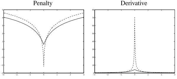
Bayesian thresholding using a NEG prior distribution is applied to a problem in immunology. The study measured gene expression level for 755 genes of known function for two groups of patients. A rheumatoid arthritis (RA) group with 24 subjects and a osteoarthritis (OA) group with 7 subjects. Three expression level measurements were taken for each sample and averaged to reduce noise-levels. The data was previously analysed in Sha et al (2003) and the interested reader is referred to this paper for a more detailed description of the experiments. The value of the λ parameter set to be 0.1 of the NEG distribution were chosen with the “typical” value of a non-zero regression coefficient) set to 2 andk0 set to be 5 and 2.5. Here we will not attempt an exploration of sensitivity to hyperparameter choicesλandk0 nor the model’s application to other datasets.

Figure 8 shows the form of the penalty function and its derivative (which controls the amount of shrinkage) for the two choices of hyperparameter,k0 _{= 5solid line andk}0 _{= 2.5}

dotted.

Penalty Derivative

−3 −2 −1 0 1 2 3 −3

−2 −1 0 1 2 3 4 5

−30 −2 −1 0 1 2 3 10

20 30 40 50 60 70 80

Figure 8: The penalty functionp(_|β_|),and its derivative for the two choices of hyperparameter,

k0 = 5(solid),k0 = 2.5dotted

For both hyperparameter settings, the EM algorithm was started at 100 randomly chosen initial values of the regression coefficients. 89 and 60 distinct modes were found fork0 _{= 5}

and k0 _{= 2.5 respectively. The posterior distribution of β is highly multi-modal with}

seemingly no overall dominating mode in both cases. Figure 9 shows the empirical cdf of

log[π(y_|βˆ)π( ˆβ)]when k0 _{= 5,2.5 for all the local posterior modes found and also the log}

k= 5 k0 = 2.5

0 10 20 30 40 50 60 70 80 90 −472

−471 −470 −469 −468 −467 −466 −465

0 10 20 30 40 50 60 1610

1612 1614 1616 1618 1620 1622

0 1 2 3 4 5 6

−9 −8 −7 −6 −5 −4 −3

0 1 2 3

−16 −14 −12 −10 −8 −6 −4

Figure 9: The top row shows plots of ranked values of log[π(y_|βˆ)π( ˆβ)] for the distinct values of the modes found and the bottom row show the values of the log likelihood for each mode (unsorted) as a function number of selected genes

is associated with the model using no genes which has a log likelihood of₋16.5589. Clearly many of the modes found have roughly similar posterior density values. Although, we would still like to express a preference for models including smaller numbers of regressors. Figures 10,11 show the actual genes chosen fork0 = 2.5,5.Figure 12 shows the regressors whose estimated coefficients are non-zero in the top ten modes ranked by their posterior density values with labels of selected genes on the x-axis. This posterior density includes the value of the penalty function and penalises less parsimonious models. Reducing the value ofk0 to 2.5 leads, unsurprisingly, to sparser models. Several of the genes appeared in both figures and in particular, the genes 290 appears in the top 3 modes. The data for the included variables with the dividing hyperplane (the locus of points for which the probability of membership to the two groups is equal withk0 _{= 2.5) are shown in figure 13. This suggests that 290 has}

substantial power to distinguish between the two disease categories.

asso-49 258 290 324 473 498 539 547 584 742 −10.7755

−10.3802 −10.2729 −10.1407 −10.0867 −9.5779 −9.03135 −8.74386 −7.08132 −7.05082

26 170 258 290 324 478 498 539 547 584 623 729 754 −6.18405

−5.91331 −5.77139 −5.00915 −4.71788 −4.54012 −4.38016 −4.14537 −3.11986 −2.38895

22 178 412 424 512 528 550 557 581 −8.9515

−7.77066 −4.57044

(a) (b) (c)

Figure 10: The log likelihood for the top modes withk0 _{= 2.5which include: (a) 1 variable, (b)}

2 variables and (c) 3 variables

83 170 178 258 290 392 478 547 584 665 729 754 −5.90622

−5.79664 −5.38688 −4.95054 −4.87581 −4.79763 −4.21331 −3.01589 −2.27097 −2.24557

26 49 54 83 84 89 115 178 192 258 290 392 404 424 461 473 478 498 528 532 649 729 −3.1974

−3.18834 −2.98045 −2.89155 −2.73436 −2.64976 −2.56393 −2.4426 −2.4088 −2.37704

(a) (b)

615 22 26 49 65 89 151 170 178 290 295 336 404 424 473 490 512 528 530 532 547 550 551 584 623 634 665 670 687 754 −4.91294

−4.30518 −4.27697 −4.17476 −3.77627 −3.65867 −3.65813 −3.20677 −3.07194 −2.41019

15262945506078 115 178 204 284 325 392 404 424 479 491 496 511 528 547 551 581 584 649 665 670 689 702 754 −7.55856

−7.13674 −5.90633 −4.96527 −4.82426 −4.7993 −4.39365 −3.78928 −3.34636

(c) (d)

Figure 11: The log likelihood for the top modes withk0 _{= 5which include: (a) 2 variable, (b) 3}

k0= 5 k0 = 2.5

26 83 89 170178258290392424478532649665729754 10 9 8 7 6 5 4 3 2 1

26 49 170 258 290 473 498 539 547 754 10 9 8 7 6 5 4 3 2 1

Figure 12: A summary of the ten modes with the highest posterior density values found by the algorithm

0 0.5 1 1.5 2 2.5 3 −1.3 −1.2 −1.1 −1 −0.9 −0.8 −0.7 −0.6 −0.5 −0.4 290 729

0 0.5 1 1.5 2 2.5 3 −0.9 −0.8 −0.7 −0.6 −0.5 −0.4 −0.3 −0.2 −0.1 290 754

0 0.5 1 1.5 2 2.5 3 −0.8 −0.6 −0.4 −0.2 0 0.2 0.4 290 170

Figure 13: Plot of the gene expression levels for two genes for the rheumatoid arthritis group (dots) and the osteoarthritis group (crosses) with the fitted dividing hyperplane

ciated with a higher chance of membership of the osteoarthritis group. Gene 290 is coding for a B lymphocyte-specific gene and clearly is very strongly associated with disease class in this very small data set. It also came to the fore in the MCMC approach of Sha et al (2003).

k0= 5 k0 = 2.5

26 83 89 170178258290392424478532649665729754 −5 −4 −3 −2 −1 0 1 2 3 4 5

26 49 170 258 290 473 498 539 547 754 −5 −4 −3 −2 −1 0 1 2 3 4 5

Figure 14: Modal regression parameter estimates for each gene

singly and in combination.

5

Discussion

In this paper we have proposed a class of prior distributions suggestive of a population of coefficients many of which are zero or near zero. By focusing on the modes of the posterior through an EM algorithm we are able to develop a method that does not search subsets but can produce coefficients that are exactly zero, much in the spirit of the original lasso. Our preferred prior is a member of the class of scale mixtures of normals, the normal-exponential-gamma (NEG), which allows a spike at zero which is not infinite and is proper over its full range. It retains some of the strong thresholding properties of the normal-Jeffreys with weak shrinkage for large coefficients without its evident overpowering drawback of impropriety of both prior and posterior.

We have compared the thresholding properties of several differing choices of prior in the scale mixture of normal class, illustrating the shape of regions in two dimensions. In higher dimensions these are harder to characterise although formulae are provided. In cases of more variables,k, than observations,n, as in the microarray example, then only min(n, k)

coefficients can be non-zero.

We have developed an EM algorithm strategy to find modal estimates. Convergence is an issue with the latent variable probit model where information in the likelihood is weaker than in the linear regression model. One arm of our strategy powers up the likelihood whilst the other updates selectively within EM. Direct maximisation of the posterior utilising Newton-Raphson with EM as in Kiiveri (2003) would be an alternative worth exploring in the con-text of generalised linear modelling. Our algorithm uses the singular value decomposition to reduce the dimensions of coefficient space whilst retaining full information content and thresholding on the original coefficients rather than those derived.

The modal analysis quantifies the posterior probabilities of coefficients being outside of a near-zero region and uses these to select interesting variables. We are also able to look at variables in combination.

References

Abramowitz, M. and Stegun, I. A. (Eds.) (1964) “Handbook of Mathematical Functions with Formulas, Graphs and Mathematical Tables,” Dover: New York.

Akaike, H. (1974): “A new look at the statistical identification model,” IEEE Transactions on Automatic Control, 19, 716-723.

Albert, J. and Chib, S. (1993): “Bayesian Analysis of Binary and Polychotomous Response Data,” Journal of the American Statistical Association, 88, 669-679.

Bae, K. and Mallick, B. K. (2004): “Gene selection using two-level hierarchical Bayesian model,” Bioinformatics, 20, 3423-3430.

Barndorff-Nielsen, O. E. and Blaesild, P. (1981): “Hyperbolic distributions and ramifica-tions: contributions to the theory and applications,” in Statistical Distributions in Sci-entific Work, Vol. 4 C. Taillie, G. Patil and B. Baldessari (ed.): , Reidal : Dorderecht.

Bernardo, J. M. and Smith, A. F. M. (1994): “Bayesian Theory,” Wiley : Chichester. Bibby, B. M. and Sorensen, M. (2003): “Hyperbolic Processes in Finance, in Handbook of

Heavy Tailed Distributions in Finance S. Rachev (ed.): , Elsevier Science, 211-248.

Box, G. E. P. and Tiao, G. C. (1973) “Bayesian Inference in Statistical Analysis,” Wiley: New York.

Breiman, L.(1996): “Heuristics of instability and stabilization in model selection,” Annals of Statistics, 24, 2350-238 .

Brown, P. J., Vannucci, M. and Fearn, T. (1998): “Multivariate Bayesian variable selection and prediction,” Journal of the Royal Statistical Society B, 60, 627-641.

Brown, P. J., Vannucci, M. and Fearn, T. (2002): “Bayes model averaging with selection of regressors,” Journal of the Royal Statistical Society B, 64, 519-536.

Dempster, A. P., Laird, N. M. and Rubin, D. B. (1977): “Maximum-likelihood from in-complete data via the EM algorithm,” Journal of the Royal Statistical Society B, 39, 1-38.

Fan, J. and Li, R.Z. (2001): “Variable selection via nonconcave penalized likelihood and its oracle properties,” Journal of the American Statistical Association, 96, 1348-1360. Fan, J. and Peng, H. (2004): “Nonconcave penalized likelihood with diverging number of

parameters,” Annals of Statistics, 32, 928-961.

Figueiredo, M. A. T. (2003): “Adaptive sparseness for supervised learning,” IEEE Transac-tions on Pattern Analysis and Machine Intelligence, 25, 1150-1159.

Foster, D. P. and George, E. I. (1994): “The risk inflation criterion for multiple regression,” Annals of Statistics, 22, 1947-75.

Gelfand, A. E. and Sahu, S. K. (1999): “Identifiability, improper priors, and Gibbs sampling for generalised linear models.” Journal of the American Statistical Association, 94, 247-253.

George, E. I. and McCulloch, R. E. (1997): “Approaches for Bayesian variable selection,” Statistica Sinica 7, 339-373.

Gradshteyn, I. S. and Ryzik, I. M. (1980) “Tables of Integrals, Series and Products: Cor-rected and Enlarged Edition,” (A. Jeffrey, Ed.) Academic Press: New York.

Johnstone, I. M. and Silverman, B. W. (2005): “Empirical Bayes selection of wavelet thresholds,” Annals of Statistics, to appear.

Kiiveri, H. (2003): “ A Bayesian approach to variable selection when the number of vari-ables is very large,” In Goldstein, D.R. (Ed) “Science and Statistics: Festschrift for Terry Speed” Institute of Mathematical Statistics Lecture Notes-Monograph Series, Vol 40, 127-143.

Knight, K. and Fu, W. (2000) “Asymptotics for lasso-type estimators”, Annals of Statistics, 28, 1356-1378.

Liu, C. H., Rubin, D. B. and Wu, Y. N. (1998): “Parameter expansion to accelerate EM: The PX-EM algorithm,” Biometrika, 85, 755-770.

Liu, J. S. (2001): “Monte Carlo Strategies in Scientific Computing,” Springer: New York. MacKay, D. J. C. (1994): “Bayesian methods for back-propagation networks,” In Domany,

E. et al (Eds) “Models of Neural Networks III” Chapter 6, 211-254.

McLachlan, G. J. and Peel, D. (2000): “Finite Mixture Models,” Wiley: New York.

Mallick, B. K., Ghosh, D. and Ghosh, M. (2005): “Bayesian classification of tumours by using gene expression data,” Journal of the Royal Statistical Society B, 67, 219-234. Meng, X. L., van Dyk, D. A. (1997): “The EM algorithm – an old folk song sung to a fast

new tune (with discussion),” Journal of the Royal Statistical Society B, 59, 511-567. Mitchell, T.J. and Beauchamp, J. J. (1988): “Bayesian variable selection in linear regression

(with Discussion),”Journal of the American Statistical Association, 83, 1023-1036. Schwarz, G. (1978): “Estimating the dimension of a model,” Annals of Statistics, 6,

Sha, N., Vannucci, M., Brown, P. J., Trower, M. K., Amphlett G., Falciani F. (2003): “Gene selection in arthritis classification with large-scale microarray expression pro-files.” Comparative and Functional Genomics, 4, 171-181.

Tibshirani, R. (1996): “Regression shrinkage and selection via the lasso,” Journal of the Royal Statistical Society B, 58, 267-288.

Tipping, M. E. and Faul, A. (2003): “Fast marginal likelihood maximisation for sparse Bayesian models,” In Frey, B. and Bishop, C. M. (Eds) Proceedings 9th International Workshop on Artificial Intelligence and Statistics, Key West, Florida.

Ueda, N. and Nakano, R. (1995): “Deterministic annealing variants of EM,” In G. Tesauro, D. S. Tourestzky, T. K. Leen (Eds) Advances in Neural Information Processing Systems 7, 545-552, MIT Press.

Vidakovic, B. (1998): “Wavelet-Based Nonparametric Bayes Methods,” in Practical Non-parametric and SemiNon-parametric Bayesian Statistics D. Dey, P. Muller and D. Sinha (eds.):, New York : Springer-Verlag, 133-156.

West, M. (2003): “Bayesian Factor regression models in the largep, smallnparadigm,” In Bernardo J. M. et al (Eds), “Bayesian Statistics 7”, 733-742: Clarendon Press: Oxford. West, M. (1987): “On scale mixtures of normal distributions. Biometrika, 74, 646-648. Wolfe, P. J., Godsill, S. J. and Ng, W. J. (2004): “Bayesian variable selection and

regulari-sation for time-frequency surface estimation,” Journal of the Royal Statistical Society, B , 66, 575-589.

Zhang, S. and Jin, J. (1996): “Computation of Special Functions,” Wiley : New York.

Appendix 1

For the lasso and simple regression, equation (13) has a turning point if_|βˆ_|> _γ1 nσ2 i=1x2i

at the point

˜

β = ˆβ₋sign( ˆβ)1

γ σ2

Pn

i=1x2i

(18)

which is also the Bayesian threshold since

logπ( ˜β_|y)₋logπ(0_|y) =₋ 1 2σ2

" ˜

β2

n

X

i=1

x2_{i −}2 ˜β

n

X

i=1

xiyi

#

−_γ1|β˜_|

=₋ Pn

i=1x2i

2σ2

˜

β2₋2 ˜ββˆ+ 2 σ

2

Pn

i=1x2i

1

γ|β˜|

and substituting in equation (18) and noting that sign

˜

β=sign

ˆ

βgives

logπ( ˜β_|y)₋logπ(0_|y) =₋ Pn

i=1x2i

2σ2

˜

β2₋2 ˜β2₋21

γ σ2

Pn

i=1x2i

˜

βsign( ˜β) + 2 σ

2

Pn

i=1x2i

1

γ|β˜|

= Pn

i=1x2i

2σ2 β˜ 2_>0.

Appendix 2

The region of different types of thresholding with a lasso penalty and two variables can be derived in the following way. The assumed form ofXTXimplies that

(XTX)−1 = 



1

c(1−ρ2₎

ρ

(1−ρ2₎√_cd

ρ

(1−ρ2₎√_cd

1

d(1−ρ2₎ 



and equation (13) can be re-arranged to give

1

c ∂L ∂β1

=β1−βˆ1+

1

csign(β1)

1

γ +

r

d

cρ( ˆβ2−β2)

and

1

d ∂L ∂β2

=β2−βˆ2+

1

dsign(β2)

1

γ +

r

c

dρ( ˆβ1−β1).

If a mode exists with both parameters non-zero, the following conditions must hold

0 =sign(β1)|β1| −βˆ1+

1

csign(β1)

1

γ +

r

d

cρ( ˆβ2−β2)

and

0 =sign(β2)|β2| −βˆ2+

1

dsign(β2)

1

γ +

r

c

dρ( ˆβ1−β1).

Some algebra gives the expression.

|β1|=sign(β1) ˆβ1−

1

γ√c

1 1₋ρ2

1

√_c +_√ρ

dsign(β1)sign(β2)

and

|β2|=sign(β2) ˆβ2−

1

γ√d

1 1₋ρ2

1

√ d+

ρ

√_csign(β1)sign(β2)

Since the right-hand side of both expression is greater than zero,

sign(β1) ˆβ1 >

1

γ√c

1 1₋ρ2

1 √ c+ ρ √

dsign(β1)sign(β2)

and

sign(β2) ˆβ2 >

1

γ√d

1 1₋ρ2

1 √ d + ρ √

csign(β1)sign(β2)

So, the regions where neither parameter is thresholded take the form of four squares. The regions where one parameter is thresholded are bounded by the four disjoint squares and the lines

ˆ

β2 =

1

√ d

ρ √_ccβˆ1+

sign(β2)

√ d

1

γ

for the region whereβ1is thresholded and

ˆ

β1=

1 √ c ρ √ dd ˆ

β2+sign

(β1)

√ c

1

γ

for the region whereβ2 is thresholded. These lines cross at the corners of the region where

both variable are thresholded. Ifcanddare equal, the graph is symmetric in the linesy =x

andy =₋x. The region where both regressor is thresholded forms a rhomboid whose shape changes with the value ofρ. The volume of the region will be determined by the ratios _γ√1_c

and 1

γ√d.

If the sum of squares for the two variables (candd) are not equal, the shape of the region where both regressors are thresholded can be less regular. The shape is a closed figure except if

1

γ√c

1 1₋ρ2

1 √ c + ρ √

dsign(β1)sign(β2)

<0

or

1

γ√d

1 1₋ρ2

1 √ d+ ρ √

csign(β1)sign(β2)

<0

ρsign(β1)sign(β2)<−

r

d

c, ρsign(β1)sign(β2)<−

r

c d

This condition reduces to

ρsign(β1)sign(β2)<−

s

min_{c, d_}

max_{c, d_}

Appendix 3

Here we derive results for normal exponential gamma distribution for (i) the marginal distribution ofβ (ii) the derivative of its form as a penalty function and (iii) the form of the E-step for it. ¿From Gradshtein Ryzik (1980, p319)

Z ∞

0

xν−1(x+β?)−ν+1/2exp_{−µx_}dx= 2ν−1/2Γ(ν)µ−1/2exp_{β?µ/2_}D1−2ν(

p 2β?_µ)

(19) Z ∞

0

xν−1(x+β?)−ν−1/2exp_{−µx_}dx= 2νΓ(ν)β?−1/2exp_{β?µ/2_}D₋2ν(

p 2β?_µ)