Optimization and redesign of actuators for a medical device

Optimization and redesign of

actuators for a medical device

e

Noor (E.M.J.) Ooms

Internship report at DEMCON

May 2016

Supervisors:

Dr.Ir. D. van de Belt (UTWENTE) Dr. Ir. D. Tjepkema (DEMCON)

Department Biomechanical Engineering University of Twente

P.O. Box 217 7500 AE Enschede The Netherlands

Faculty of Engineering

3

Abstract

Demcon is developing custom designed actuators for a medical company which are used in a therapeutic vest worn by patients who suffer from cystic fibrosis. The actuators create oscillating forces in a predetermined force profile on the patient’s thorax that helps to loosen the mucus in the lungs. This can be coughed up at a later stage. The current design of the actuator has magnets to create force with the current through the coil, and leaf springs that cause pretension and linear guidance of the back iron.

A sensitivity analysis on the influence of variations in the actuator parameters on the therapy force is performed. These actuator parameters are: mass of the moveable body, stiffness of the springs that are used to connect the moveable body to the static part of the actuator, coil resistance, coil inductance, and the (position dependent) motor constant. This sensitivity analysis is done using simulations in Matlab/Simulink, and analytically using the Taylor series expansion. The

Matlab/Simulink model is optimised and the tolerances of the parameters are determined. Results were used to optimise and improve the control system of the actuator. This decreased the

dissipated power and improved the accuracy of the applied therapy force.

After that, a redesign of the actuator is made in order to lower weight. A therapeutic vest contains eight actuators of 550 grams each, which makes the vest very heavy. The main goal of the redesign is to lower weight to 350 grams per actuator and keep the other functionalities of the actuator the same. The redesign contains a ball bearing which causes linear guidance of the back iron, and helical compression springs to generate the pretension of the back iron. The new actuator is easy to assemble and has a minimum amount of components. Furthermore, the actuator is 15% smaller in volume and weighs only 331 grams.

4

Table of Content

Introduction ... 6

Chapter 1: Analysis of the actuator ... 7

1.1. Mechanical design of the actuator ... 7

1.2. Actuator requirements ... 7

1.3. Therapy force waveform generation ... 8

1.4. Engineering formulas for actuator optimisation ... 8

1.5. The model ... 9

1.6. Matlab/Simulink model ... 10

Chapter 2: Sensitivity analysis... 12

2.1. Discretisation problem... 12

2.1.1. Solution 1: Higher sample frequency ... 13

2.1.2. Solution 2: Correction factor based on function fit ... 14

2.1.3. Solution 3: Correction factor based on a look-up table ... 14

2.1.4. Solution selection ... 14

2.2. Sensitivity analysis ... 15

2.3. Analytical solution ... 17

Chapter 3: Waveform optimisation ... 19

3.1. Testing new waveforms ... 19

3.2. Optimising original waveform ... 20

Chapter 4: Verifying the assumed rigid thorax ... 22

Chapter 5: Redesign of the actuator ... 24

5.1. Reduction of the motor parameters and therapy parameters ... 24

5.2. Functional design in FEMM ... 25

5.3. Morphological diagram ... 27

5.3.1. Pretension ... 28

5.3.2. Linear guidance ... 31

5.3.3. Elimination ... 34

5.4. Concepts... 34

5.4.1. Concept 1: compression-extension springs with ball bearing ... 34

5.4.2. Concept 2: compression springs with ball bearing ... 36

5.4.3. Concept 3: compression springs with elastic bearing ... 37

5.4.4. Concept 4: membrane spring ... 38

5.4.5. Summary of the concepts ... 39

5.5. Selection of the concepts ... 39

5.6. Final concept ... 40

5

5.6.2. Optimization and adjustments ... 41

5.6.3. Detailed design ... 42

5.6.4. Moving actuator ... 44

Conclusions ... 45

References ... 46

Appendices ... 47

Appendix A: results measurements prototypes ... 47

Appendix B: derivation transfer function ... 48

Appendix C: Mass analysis of the concepts and final design ... 49

6

Introduction

Demcon is developing custom designed actuators for a medical company. The actuators are used in a vest worn by patients who suffer from cystic fibrosis. The actuators create oscillating forces on the patient’s thorax that helps to loosen the mucus in the lungs. This can be coughed up at a later stage.

a) b)

Figure 1: a) Prototype of the therapeutic vest, b) Transversal cross section of the prototype [1]

Oscillating forces are obtained by accelerating a moving balance mass towards and away from the patient’s thorax. The force created by this principle is called the Lorentz force. The oscillating forces have specific waveforms (force profiles) that are dependent on the preferences of the patients regarding frequency content and peak force magnitude.

Demcon has already realized a first prototype of the actuator which performs well in a prototype therapeutic vest. Three observations are made. First, for future series production it is essential to understand how variations in actuator parameters influence the waveforms and the magnitude of the therapy forces. Second, the force profile that is used in the prototype is based on an educated guess which might not be the most efficient force profile. Third, the therapeutic vest including the current design of the actuator is found heavy by the test users.

As first part of the assignment, a sensitivity analysis on the influence of variations in the actuator parameters on the waveforms is performed. These actuator parameters are: mass of the moveable body, stiffness of the springs that are used to connect the moveable body to the static part of the actuator, coil resistance, coil inductance, and the (position dependent) motor constant. This sensitivity analysis is done using simulations in Matlab/Simulink, and analytically using the Taylor series expansion. This Matlab/Simulink model needs to be optimised and the tolerances of the parameters are determined. After that, it is investigated if the force profile can be further optimised. As last part of the assignment, a redesign of the actuator is made in order to lower weight. This redesign is based on an adjusted list of requirements.

Some background information about the current design of the actuator is given in Chapter 1. After that a sensitivity analysis is performed in Chapter 2, the waveform optimisation is described in

7

Chapter 1: Analysis of the actuator

The therapeutic vest consist of eight voice coil actuators, four at the back and four at the chest of the patient. The main function of those actuators is to deliver a therapy force on the patient’s thorax according to a predefined force profile. The therapy force is delivered between a moving balance mass and the patient’s thorax. This moving mass is the moving magnet assembly of the voice coil actuator.

1.1.

Mechanical design of the actuator

After some research and calculations, a mechanical design for the actuator is made as shown in

Figure 2. This consists of a moving back iron, a ring shaped permanent magnet which is magnetised in the radial direction, and two membrane springs that connect the moving body to the static part on which a coil is placed. A voice coil actuator can deliver a force according to the Lorentz force principle. Due to a current flow in the coil, a force is created if the coil interacts with the magnetic field due to the permanent magnet. The back iron is necessary to guide the magnetic field. This magnetic field will produce a force that will move the moving body with respect to the static part with the coil.

The actuator is designed in a way to fulfil the customer requirements and of course must be safe. The coil is intended to never impact the back iron or magnet. This is realised by using rubber end stops and using a linear guidance by two membrane springs. These springs have actually two functions, act as a linear guiding of the moving body, and give the system a specific resonance frequency to keep the power consumption low.

Figure 2: Mechanical design of the voice coil actuator [1]

1.2.

Actuator requirements

The design of the voice coil actuator is based on a list of requirements from the customer. It should be small sized, low weight, low dissipated power, high impulse, low cost and of course be safe. The main requirements are listed below:

 8 actuators (4 at the chest and 4 at the back) are required.

8

 Peak therapy force must be adjustable from 3 to 30 N in steps of 3 N and must be achievable for all therapy frequencies.

 Supply voltage to the actuators is 24 V at maximum.

 Actuators are intended to be used horizontally but tilt angles up to ±30° with respect to the horizontal line are allowed.

The requirements that the actuators should be low weight and have a small dissipated power are trade-offs. If the weight is really low, the accelerations and consequently the displacement of the moving body needs to be high to be able to produce the desired force. This follows from Newton’s second law (𝐹 = 𝑚𝑎) and the relation between acceleration and displacement: 𝑥 =1

2𝑎𝑡2. A large displacement will make the vest very big and thick, which is also undesired. A good compromise between those variables is made.

1.3.

Therapy force waveform generation

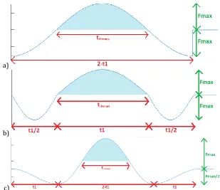
The therapy force is applied in a waveform that will give the desired therapy force at the desired therapy frequency, and is efficient. The force profile used for the actuator is shown in Figure 3. When the therapy frequency is very low, there is some waiting time (𝑡_𝑤) between the pulses. During that waiting time, the membrane springs are stretched what will cause a lot of dissipated power. To avoid this, some position correction is added to the signal. This will put the moving body back to its equilibrium position during the waiting time to decrease the dissipation as shown in

Figure 3b.

Figure 3: Waveform of the desired therapy force a) for high frequencies, b) for low frequencies

1.4.

Engineering formulas for actuator optimisation

For the design of the actuator, some basic formulas are required. The major design criterion is to optimise the actuator to achieve a high efficiency over weight ratio. The efficiency is expressed as the second power of the force in [N2_{] per Watt dissipated electrical power. Hereby can the actuator}

force 𝐹𝑎𝑐𝑡 be calculated using: 𝐹𝑎𝑐𝑡= 𝑛𝑤𝑖𝑛𝑑𝑖𝑛𝑔𝑠𝐵𝐼𝐷𝑐𝑜𝑖𝑙 and the dissipated power 𝑃 using:

𝑃 = 𝐼2_{𝑅 =}𝐹𝑎𝑐𝑡2

𝑘𝑚2 𝑅 where 𝑛𝑤𝑖𝑛𝑑𝑖𝑛𝑔𝑠 is the number of active coil windings, 𝐵 is the average magnetic

9

can be calculated using 𝑅 =4𝜌𝑛𝑤𝑖𝑛𝑑𝑖𝑛𝑔𝑠𝐷𝑐𝑜𝑖𝑙

𝑑2 and the motor constant 𝑘𝑚 using: 𝑘𝑚 =

𝐹𝑎𝑐𝑡

𝐼 =

𝑛_{𝑤𝑖𝑛𝑑𝑖𝑛𝑔𝑠}𝐵𝐷_{𝑐𝑜𝑖𝑙} where 𝜌 is the electrical resistivity of the wire material (cupper) in [m], and 𝑑 is the wire diameter. Manipulating those equations will give a relation between the copper volume in the coil and the actuator force and dissipated power: 𝑉 = 𝜋2 𝐹2𝜌

𝐵2_𝑃.

1.5.

The model

Next to those engineering formulas, a simple model describes how the actuator is able to deliver the therapy force on the patient’s thorax. The desired therapy force needs to be translated to an

electrical signal (a voltage and current) which controls the actuator. To be able to do this, a dynamic model of the actuator is considered. This is related to the current by the motor constant

(𝐹𝑎𝑐𝑡= 𝑘𝑚𝐼). This current is needed to find the voltage to control the actuator.

Figure 4: Simple model of interaction between patient’s thorax and actuator [1]

The patient’s thorax can be considered as a rigid body on which both the actuator force and the spring force that is executed by the membrane spring, are acting. These two forces are also acting on the moving assy as shown in Figure 4. This gives:

−𝐹_{𝑡ℎ𝑒𝑟𝑎𝑝𝑦}= −𝐹_𝑎𝑐𝑡− 𝑘 ∆𝑥 = 𝑚 ∆𝑥̈ (1)

With 𝐹_𝑎𝑐𝑡 the actuator force, 𝑘 is the spring constant and ∆𝑥 is the displacement.

Another point of interest is the relationship between the driving current and voltage to realize the desired therapy force. The needed voltage to realise the therapy force consists of the voltage to overcome the resistance of the wire, the voltage to overcome the inductance of the wire, and the voltage to overcome the back electromotive force (back-EMF). We get the following relation[1]_:

𝑈 = 𝑈_𝑅+ 𝑈_𝐿+ 𝑈_𝐸𝑀𝐹 (2)

Using the following expressions for the components of the voltage, this equation can be rewritten.

- The voltage caused by back-EMF, 𝑈𝐸𝑀𝐹: 𝑈𝐸𝑀𝐹 = 𝑘𝑚𝑥̇

- The voltage caused by self-inductance, 𝑈𝐿: 𝑈𝐿 = 𝐿_𝑑𝑡𝑑𝐼

- The voltage caused by resistance of the coil, 𝑈𝑅: 𝑈𝑅 = 𝐼𝑅

10

𝑈 = 𝐼𝑅 + 𝐿𝑑𝐼

𝑑𝑡+ 𝑘𝑚∆𝑥̇ (3)

1.6.

Matlab/Simulink model

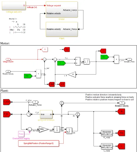
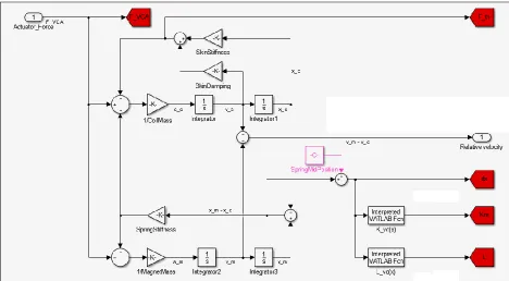
Based on the data about the designed voice coil actuator, the requirements, the engineering formulas, the model, and the force profile, a Matlab/Simulink model is made. This model is schematically shown in Figure 5 and shortly explained here.

Motor:

Plant:

11

This Matlab/Simulink model consists of three main blocks: voltage setpoint, motor, and plant. The first block, voltage setpoint, calculates the required voltage at every time step to create the desired therapy force profile. A sample frequency of 1 kHz is used, so one time step has a duration of

1/1000 second. The desired therapy force is set in the block voltage setpoint, from which the desired acceleration can be calculated (using 𝐹𝑡ℎ𝑒𝑟𝑎𝑝𝑦 = −𝑚𝑎). Integrating the acceleration gives the velocity, integrating again gives the displacement. The actuator force can be determined using

Equation (1) which is used to calculate the current (𝐼 = 𝐹_𝑎𝑐𝑡/𝑘_𝑚). Then, the voltage setpoint can be calculated using Equation (3). This is calculated for every time step and is send to the next block: motor.

The motor and plant combined represent the simulation which should give the same therapy force as set in the voltage setpoint. In the second block, motor, the calculations are executed in reverse direction. The current, and then the actuator force, is calculated from the voltages whereby the velocity comes from the plant. The simulated actuator force is output from the second block and goes to the third block, the plant.

The plant simulates the simple dynamical model as described above. This gives the velocity as output, which goes to the motor again.

12

Chapter 2: Sensitivity analysis

For the first part of the research, some questions about sensitivity are answered, and some improvements and optimisation opportunities in the model are investigated. The main aspects of the design of the actuator that are investigated are:

1. Discretisation problem: improvements on the model to make the simulated therapy force equal to the set therapy force.

2. Sensitivity analysis: the influence of some actuator parameters on the applied therapy force. Using this sensitivity analysis the worst case situation can be determined, and tolerances for the actuator parameters are set.

3. Analytical solution: comparing the simulation to the analytical results from a Taylor expansion.

2.1. Discretisation problem

The simulated therapy force applied by the actuator is in most cases higher than the therapy force set point. These deviations appear to be around the 3-4% for all settings (all combinations of 5 to 20 Hz therapy frequency and 3 to 30 N therapy force). These deviations are probably caused by the way the set point signal is generated: by discretisation of the continuous signal. This will cause deviations in the set point signal on which the simulation is based. This will also cause deviations in the simulated signal as shown in Figure 6.

Figure 6: Discretisation(red) of a continuous signal (grey) gives deviations in the set point signal

In the final product, only a deviation of 5% in the therapy force is allowed. It is not desired to have a deviation of 4% due to a non-optimised set point signal, since there will always be other deviations caused by variations in actuator parameters, influence of the body, manufacturing errors etc. So this deviation in the model should be as small as possible.

13

1. Use a higher sample frequency

2. Correct for the deviation with a correction factor based on a function fit of the 3D plot. 3. Correct for the deviation with a correction factor based on the simulated therapy force for

every possible setting. This correction factor is stored in a look-up table with the perfect correction factor for every possible setting.

The results of those three solutions are investigated and comparted to each other to select the most suitable solution.

Figure 7: 3D plot of the deviations from the therapy force set point

2.1.1. Solution 1: Higher sample frequency

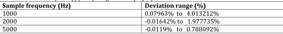
A sample frequency of 1000 Hz is used to create the set point therapy force. This will create a discrete signal which approaches a continuous signal. The higher the sample frequency, the better this continuous signal is approached and the better the simulated therapy force in the ‘plant model’ will approach the desired therapy force signal. To investigate the influence of the sample frequency on the deviations from the therapy force set point, the deviations for all possible combinations of settings are calculated for a sample frequency of 1000 Hz, 2000 Hz and 5000 Hz. The results are shown in Table 1. From these results it can be seen that increasing the sample frequency will indeed decrease the deviations from the therapy force set point.

Table 1: Deviations of therapy force for different sample frequencies

Sample frequency (Hz) Deviation range (%)

1000 0.07963% to 4.013212%

2000 -0.01642% to 1.977735%

14 2.1.2. Solution 2: Correction factor based on function fit

Using Matlab Curve Fitting Tool, an equation that fits the plot shown in Figure 7 is determined. This equation is a polynomial equation of order 3 of the form:

𝑑𝑒𝑣𝑖𝑎𝑡𝑖𝑜𝑛(𝑥, 𝑦) = 𝑝₀₀+ 𝑝₁₀𝑥 + 𝑝₀₁𝑦 + 𝑝₂₀𝑥2_{+ 𝑝}

11𝑥𝑦 + 𝑝02𝑦2+ 𝑝30𝑥3+ 𝑝21𝑥2𝑦 + 𝑝12𝑥𝑦2+ 𝑝03𝑦3

With 𝑥 the Therapy Force (N), 𝑦 is the Therapy Frequency (Hz), and 𝑝_𝑖𝑗 are constants:

p00=-0.2547; p01=0.04184; p11=-0.001511; p30=0.00004729; p12=-0.0002181; p10=0.02498; p20=0.005192; p02=-0.005853; p21=0.00008501; p03=0.0008022; This polynomial equation gives approximately the deviation of the simulated value from the set point value (R-square = 0.9716). To correct for this real deviation, this calculated deviation is subtracted from the therapy force in the Simulink model. This is done by adding a gain in the ‘Matlab/Simulink model, plant’ (Figure 5, plant). This gain is added just before the red ‘goto’-flag of ‘F_th’. The gain is equal to: 𝑔𝑎𝑖𝑛 =_{100+𝐶𝑜𝑟𝑟𝐹𝑎𝑐}100 where 𝐶𝑜𝑟𝑟𝐹𝑎𝑐 is the deviation in percentage.

With this correction factor the deviations appear to lie between -0.42988% and 0.322862% for a sample frequency of 1000 Hz. There is still a deviation present because not the real deviation is used as correction factor but the results from the Curve Fitting polynomial, which does not fit everywhere equally well.

The same procedure is used to find an equation for the correction factor (𝐶𝑜𝑟𝑟𝐹𝑎𝑐) by using a sample frequency of 2000 Hz. This gives deviations between -0.2241% and 0.1416% from the set therapy force. The deviations lie between -0.0904% and 0.055593% for a sample frequency of 5000 Hz. So applying a correction factor based on a function fit will decrease the deviations. This can be decreased even further by increasing the sample frequency.

2.1.3. Solution 3: Correction factor based on a look-up table

The deviation is calculated for every possible combination of settings. The results can be saved in a table and be used to correct for this error. This gives a 10x16 table in which the correction factors can be found for every setting. This correction factor is applied in the same way as the correction factor with the function fit in ‘Solution 2’. By applying this correction factor, the deviations are always equal to zero. This is obvious since the exact deviation is subtracted.

2.1.4. Solution selection

15

This is introduced in Matlab using some extra code where 𝑑𝑒𝑣 is the 10x16 table with the deviations:

This correction factor is implemented in the ‘Matlab/Simulink model, plant’ by using a gain:

𝑔𝑎𝑖𝑛 = 100

100+𝐶𝑜𝑟𝑟𝐹𝑎𝑐 where 𝐶𝑜𝑟𝑟𝐹𝑎𝑐 is the deviation in percentage, in front of the output F_th. This correction factor is applied to perform the sensitivity analysis to ensure that the measured deviation is only coming from variation in the parameters and not from the model anymore.

2.2. Sensitivity analysis

There are five important actuator parameters that can have deviations from the expected value. The five actuator parameters that are tested are:

1. The mass of the moving body 𝑚

2. The spring constant 𝐾

3. The resistance of the coil 𝑅

4. The motor constant 𝐾𝑚, this parameter is position dependent 5. The coil inductance 𝐿𝑚, this parameter is position dependent

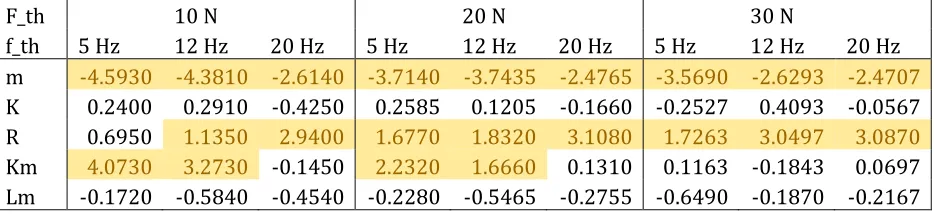
The influence of every parameter is tested individually. It is assumed that all five parameters are completely independent of each other. The Matlab/Simulink model is adapted to make it easy to add some error on the values of the parameters. This is done by introducing an error value for all of them. Every parameter is tested with a deviation of +5% and -5%. So the original value is multiplied by (1.00+0.05) or (1.00-0.05). This is done for a set therapy force of 10N, 20N and 30N, with a therapy frequency of 5Hz, 12Hz and 20Hz. The results are summarized in Table 2. It is clear that the variations in mass, the coil resistance and the motor constant cause the biggest deviations in the therapy force. These tolerances should be made as small as possible to reduce the deviations in the therapy force.

Table 2: a) Percentage deviation in therapy force due to -5% variations in the five parameters (yellow: deviation is more than ±1%)

F_th 10 N 20 N 30 N

f_th 5 Hz 12 Hz 20 Hz 5 Hz 12 Hz 20 Hz 5 Hz 12 Hz 20 Hz

m -4.5930 -4.3810 -2.6140 -3.7140 -3.7435 -2.4765 -3.5690 -2.6293 -2.4707

K 0.2400 0.2910 -0.4250 0.2585 0.1205 -0.1660 -0.2527 0.4093 -0.0567 R 0.6950 1.1350 2.9400 1.6770 1.8320 3.1080 1.7263 3.0497 3.0870

Km 4.0730 3.2730 -0.1450 2.2320 1.6660 0.1310 0.1163 -0.1843 0.0697

Lm -0.1720 -0.5840 -0.4540 -0.2280 -0.5465 -0.2755 -0.6490 -0.1870 -0.2167

CorrFac_table=load('deviations_peak2_SampleFreq1000','dev');

row=TherapyForce/3; column=TherapyFreq-4;

16

b) Percentage deviation in therapy force due to +5% variations in the five parameters (yellow: deviation is more than ±1%)

F_th 10 N 20 N 30 N

f_th 5 Hz 12 Hz 20 Hz 5 Hz 12 Hz 20 Hz 5 Hz 12 Hz 20 Hz

m 4.5970 4.1660 2.3960 3.8105 3.6105 2.6485 2.5633 3.0193 2.7020

K -0.1980 -0.4700 0.3410 -0.0815 -0.2455 0.4810 -0.5837 0.2333 0.4440 R -0.5930 -1.2280 -2.8390 -1.4665 -1.8010 -2.6195 -2.5107 -2.2803 -2.5473

Km -3.9870 -3.3640 -0.3050 -1.9545 -1.8965 -0.2170 -1.2877 0.1130 -0.1287

Lm 0.3020 0.3970 0.3290 0.3495 0.4495 0.5525 -0.2417 0.7440 0.5643

From the results in Table 2, the worst case for every parameter is determined. By applying the worst case for every parameter, the worst case for the whole model can be determined (it is assumed that all the parameters are independent of each other). These results are shown in Table 3

where the percentages are the deviations of the simulated therapy force from the set therapy force.

Table 3: Percentage deviation in therapy force in the worst cases

10 N 20 N 30 N 5 Hz 10.0694% 8.2854% 5.8646% 12 Hz 9.8557% 7.8620% 6.6839% 20 Hz 6.2159% 6.4597% 6.3379%

The maximum allowable deviation in the therapy force is 5%, so the tolerances of the five parameters are investigated to see what the real deviations for every separate parameter are.

The standard deviation for every parameter is determined using the test results of 20 prototypes of the actuator, see Appendix A. The mean value 𝜇 and the standard deviation 𝜎 are determined for the resistance R, and the eigenfrequency 𝜔𝑟. The deviation in the parameters is set to 3𝜎 which covers 99.73% of the cases and can be calculated by: 𝑑𝑒𝑣 = 3𝜎/𝜇. The variation in the spring constant can be calculated using the eigenfrequency: 𝐾 = 𝑚(2𝜋𝜔_𝑟)2 _{where 𝑚 is the mass of the moving body.}

The results are shown in Table 4. Here are the motor constant 𝐾𝑚 and the inductance 𝐿𝑚 a function of the displacement 𝑥, so these do not have a mean value and a standard deviation, but they got a deviation based on the curves as shown in Appendix A.

Table 4: Deviations in the parameters based on research on prototypes

Parameter Mean value 𝝁 Standard deviation 𝝈 Deviation worst case

m 0.387 kg - 1%

ωr 12.440 s-1 0.1659 s-1 -

K 2364.3 N/m 64.0726 N/m 8.05%

R 3.8655 Ω 0.0332 Ω 2.57%

Km - - 5%

17

The deviations as shown in Table 4 are used to determine the worst case deviation in the therapy force again. The results are shown in Table 5 which shows that mainly the combination of a low therapy frequency and a low therapy force gives too high deviations.

Table 5: Percentage deviation in therapy force in the worst cases based on prototype results

3 N 12 N 21 N 30 N

5 Hz 7.7205% 5.3355% 3.8673% 2.5909%

12 Hz 5.5932% 5.4952% 3.5212% 2.3394%

20 Hz 2.7280% 2.7808% 2.7559% 2.5430%

After some trial and error by adjusting the tolerances, it can be concluded that it is not possible to decrease these tolerances and to get the deviation of the therapy force lower than 5% for all combinations of therapy frequency and therapy force. This gives the final and best tolerances as shown in Table 4.

2.3. Analytical solution

The influence of the five parameters can not only be tested in the simulation, but also using a Taylor series expansion. First the transfer function is derived (see Appendix B for the full derivation):

𝐺(𝑠) =𝐹𝑡ℎ(𝑠)

𝑈(𝑠) =

𝑘𝑚𝑚𝑠2

(𝑅+𝐿𝑚𝑠)(𝑚𝑠2+𝑘)+𝑘𝑚2𝑠 (4)

A Taylor series expansion is performed with respect to the five parameters 𝑚, 𝑘, 𝑅, 𝑘_𝑚 and 𝐿_𝑚

around their nominal values (𝑚0, 𝑘0, 𝑅0, 𝑘𝑚0, 𝐿𝑚0). A Bode diagram is made for each parameter which will give insight in the sensitivity of the therapy force on those parameters. This should give a result similar to the sensitivity analysis as described before.

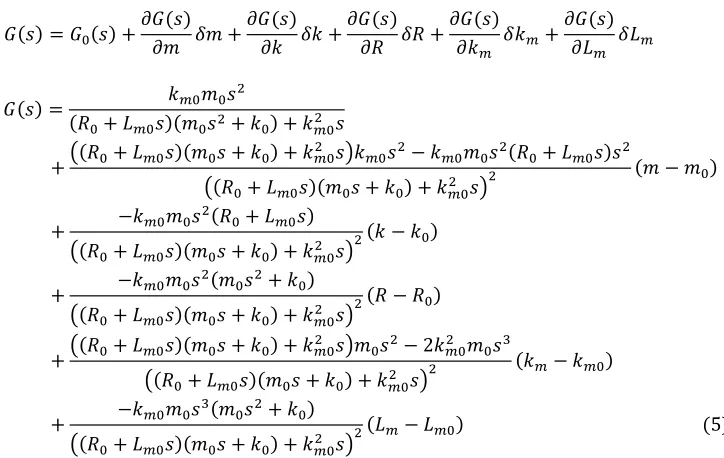
The total derived Taylor series expansion is:

𝐺(𝑠) = 𝐺0(𝑠) +𝜕𝐺(𝑠) 𝜕𝑚 𝛿𝑚 +

𝜕𝐺(𝑠) 𝜕𝑘 𝛿𝑘 +

𝜕𝐺(𝑠) 𝜕𝑅 𝛿𝑅 +

𝜕𝐺(𝑠) 𝜕𝑘𝑚 𝛿𝑘𝑚+

𝜕𝐺(𝑠) 𝜕𝐿𝑚 𝛿𝐿𝑚

𝐺(𝑠) = 𝑘𝑚0𝑚0𝑠 2

(𝑅0+ 𝐿𝑚0𝑠)(𝑚0𝑠2+ 𝑘0) + 𝑘𝑚02 𝑠

+((𝑅0+ 𝐿𝑚0𝑠)(𝑚0𝑠 + 𝑘0) + 𝑘𝑚0

2 _{𝑠)𝑘𝑚0𝑠}2_{− 𝑘𝑚0𝑚0𝑠}2_{(𝑅0+ 𝐿𝑚0𝑠)𝑠}2

((𝑅0+ 𝐿𝑚0𝑠)(𝑚0𝑠 + 𝑘0) + 𝑘𝑚02 𝑠)

2 (𝑚 − 𝑚0)

+ −𝑘𝑚0𝑚0𝑠

2_(𝑅

0+ 𝐿𝑚0𝑠) ((𝑅0+ 𝐿𝑚0𝑠)(𝑚0𝑠 + 𝑘0) + 𝑘𝑚02 𝑠)

2(𝑘 − 𝑘0)

+ −𝑘𝑚0𝑚0𝑠2(𝑚0𝑠2+ 𝑘0) ((𝑅0+ 𝐿𝑚0𝑠)(𝑚0𝑠 + 𝑘0) + 𝑘𝑚02 𝑠)

2(𝑅 − 𝑅0)

+((𝑅0+ 𝐿𝑚0𝑠)(𝑚0𝑠 + 𝑘0) + 𝑘𝑚02 𝑠)𝑚0𝑠2− 2𝑘𝑚02 𝑚0𝑠3 ((𝑅0+ 𝐿𝑚0𝑠)(𝑚0𝑠 + 𝑘0) + 𝑘𝑚02 𝑠)

2 (𝑘𝑚− 𝑘𝑚0)

+ −𝑘𝑚0𝑚0𝑠

3_(𝑚0𝑠2_{+ 𝑘0)}

((𝑅0+ 𝐿𝑚0𝑠)(𝑚0𝑠 + 𝑘0) + 𝑘𝑚02 𝑠)

18

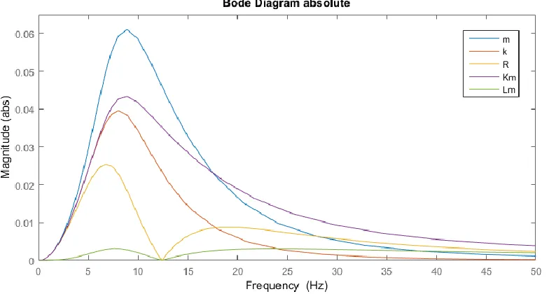
For every transfer function belonging to one of the parameters, a Bode diagram is made and scaled to the nominal value of this parameter. The magnitude plot is shown in Figure 8. The deviation in therapy force per voltage due to a variation of 5% in every parameter is shown. These deviations are at a maximum for a frequency around 7-8 Hz.

Figure 8: Magnitude plot of the Taylor series expansions; |𝜕𝐺0(𝑠)/𝜕𝑚|/𝑚0 (blue), |𝜕𝐺0(𝑠)/𝜕𝑘|/𝑘0 (red),

|𝜕𝐺0(𝑠)/𝜕𝑅|/𝑅0 (yellow), |𝜕𝐺0(𝑠)/𝜕𝑘𝑚|/𝑘𝑚0 (purple) and |𝜕𝐺0(𝑠)/𝜕𝐿𝑚|/𝐿_𝑚0(green)

From this analytical analysis, it can be concluded that the influence of the inductance of the coil is very small and the influence of the mass is the biggest. This is similar to the result from the

19

Chapter 3: Waveform optimisation

A waveform is introduced in Chapter 1. This waveform gives good results, but it has not been investigated what other waveforms do and what the best way is to add a position correction to the waveform. These two aspects of the waveform are investigated.

3.1.

Testing new waveforms

For the cases with higher therapy frequencies, the position correction is not applied. Three other waveforms are investigated for these situations and the results are compared to the original waveform. These other waveforms are shown in Figure 9. For the therapies at low frequencies, the original position correction is adjusted to get the best result by adjusting the amplitudes of the peaks. Also, another simple way of position correction is investigated and compared to the original optimised position correction. This simple position correction is created by adding a sinus in front of the acceleration signal of the acceleration. This will cause the magnet to move back to its

equilibrium position at 5 mm. This is shown in Figure 10 together with the original position correction.

The results of the waveform are compared to each other on a few factors. First, the displacement ∆x must be within acceptable ranges. Second, the impulse (i.e. the integral of the positive part of the therapy force over time) must be as big as possible. This is reached when the therapy time ttherapy is

as long as possible. This therapy time is the time duration of the positive part of the therapy force. Third, the power dissipation must be kept small. Based on this, the most efficient waveform is selected.

a)

b)

c)

20

a)

b)

Figure 10: Position correction for the original waveform a) original position correction b) simple position correction

The four waveforms (the original and the three new waveforms) are tested at a therapy frequency of 5 Hz and 20 Hz. For the 20 Hz simulations there is no position correction applied and for the 5 Hz simulations the simple position correction is applied. The results are shown in Table 6. All

waveforms create displacement within the boundaries. The original waveform and waveform 3 show similar and the lowest dissipated power for both therapy frequencies.

Table 6: waveform analysis

Original Waveform 1 Waveform 2 Waveform 3 5 Hz

(simple PosCorr) Pttherapydiss (W) (s)

∆x (mm)

1.0283 W 0.0199 s 1 – 9 mm

1.6205 W 0.0226 s 1 – 9 mm

1.7601 W 0.0239 s 1 – 9 mm

1.1562 W 0.0171 s 1 – 9 mm 20 Hz

(Without PosCorr)

Pdiss (W)

ttherapy (s)

∆x (mm)

2.2553 W 0.0167 s 2 – 8 mm

4.2198 W 0.0226 s 1 – 9 mm

5.1077 W 0.0239 s 1 – 9 mm

2.4472 W 0.0167 s 3 – 7 mm

3.2.

Optimising original waveform

The original waveform had a position correction with a sine with amplitude 𝑎𝑚𝑎𝑥/2 but the displacement is not within the boundaries (the moving assy will touch the end stops). The amplitude and the period of this sine can be optimised to get the best allowable results. The durations of the three peaks, as defined in Figure 3, and the amplitudes of the three peaks are dependent of each other whereby the amplitude of the peak that causes the therapy force is set. The others can be determined using some boundary conditions:

- At time 𝑡 = 𝑡3+ 𝑡2 (at the start of the therapy peak) the acceleration should be equal to zero for both cases, with and without position correction. So the velocity and the displacement of the moving body with position correction should be equal to respectively the velocity and the displacement without position correction.

- At the point where the velocity is equal to zero, the displacement should be equal to its

21

The amplitude 𝑎𝑚𝑎𝑥 of the therapy peak is set and 𝑡𝑡ℎ𝑒𝑟𝑎𝑝𝑦 is determined. Using this, a system of three equations with four variables and multiple solutions is obtained. Two of the other variables can be chosen to solve the system of equations, this is done by choosing one variable and iterating a second until the best result is obtained.

The best result for the original waveform is obtained for:

Here is the amplitude of the peak during 𝑡₃ equal to 𝑎𝑚𝑎𝑥/𝑛 and the amplitude of the peak during

𝑡₂ equal to 𝑎𝑚𝑎𝑥/𝑚 as shown in Figure 11. This result shows that the original waveform using the optimised position correction can be improved even more. The dissipated power is equal to 0.9709 W for a therapy frequency of 5 Hz and the moving assy moves within the boundaries now.

From this it can be concluded that the original waveform with the optimised version of the position correction gives the best results. The dissipation is the lowest, and 𝑡_{𝑡ℎ𝑒𝑟𝑎𝑝𝑦} is bigger than for waveform 3, so the impulse will be higher. The moving body will also stay within the boundaries and is able to move safely in the actuator without touching the end stops.

Figure 11: Force profile with amax as measure for the magnitude of the force

m = 1.72167; % amplitude factor during t2

n = 2.0; % amplitude factor during t3

a = -2.0/m-2.0*n/m/m; b = 2.0*t1+2.0*t1*n/m;

22

Chapter 4: Verifying the assumed rigid thorax

In the model it is assumed that the thorax is a rigid body which is not the case in reality. A new model is made which also included the effects of the body. The tissue is modeled as a spring and a damper. The weight of the tissue and the stationary part of the actuator together is called 𝑚𝑐, and the moving part of the actuator is 𝑚_𝑚. The dynamic model is shown in Figure 12 and expressed in

Equation (6). The Matlab/Simulink model is adjusted to this dynamic model by modeling Equation (6) in the ‘Plant’ in Simulink as shown in Figure 13.

{ _−𝑘𝑘𝑠𝑝𝑟𝑖𝑛𝑔(𝑥𝑚− 𝑥𝑐) + 𝐹𝑎𝑐𝑡− 𝑘𝑠𝑘𝑖𝑛𝑥𝑐− 𝑐𝑠𝑘𝑖𝑛𝑥̇𝑐= 𝑚𝑐𝑥̈𝑐

𝑠𝑝𝑟𝑖𝑛𝑔(𝑥𝑚− 𝑥𝑐) − 𝐹𝑎𝑐𝑡 = 𝑚𝑚𝑥̈𝑚 (6)

Figure 12: Dynamic model with compliant tissue

Figure 13: Adjusted ‘Plant’ in the Matlab/Simulink model

23

age, gender, body mass index, types and percentages of tissue in the tissue layer, hydration, thickness of the tissue layer, and location on the body.

An approximation for the mass of the tissue is made using the diameter of the actuator (7

centimeters), a thickness of 1 centimeter tissue and a density of tissue of 1050 kg/m3_{. This gave a}

mass of the tissue of 40 grams. The mass of the stationary part of the actuator is 150 grams according to the original Matlab/Simulink model. This gives a total mass of 190 grams for 𝑚_𝑐.

It is known that tissue causes an overdamped system, so the damping ratio ζ (zeta) has to be bigger than one: 𝜁 > 1. According to Amar M.R.S. [2] _{the damping constant has a value of 𝑐𝑠𝑘𝑖𝑛 = 1.824 and}

the spring stiffness 𝑘_{𝑠𝑘𝑖𝑛}= 18500 𝑁/𝑚. This gives a good order of magnitude to start the

simulations. The influence of the damping ratio and the stiffness on the simulated therapy force is investigated by varying these parameters. The damping ratio is varied between 1 and 2. This showed a smaller range of deviations in the simulated therapy force from the set therapy force for higher damping ratios. This also caused a small increase in dissipated power. The stiffness of the tissue is varied between 750 N/m and 150000 N/m. This showed smaller deviations and higher dissipated power for stiffer material (higher stiffness).

All deviations of the simulated therapy force are negative, so the actual applied force is less than desired. For all tested damping ratios and stiffness higher than 10000 N/m, this deviation is always smaller than 5%, as shown in Figure 14. Also the dissipated power stays low as shown in Figure 14. If the thorax has a stiffness higher than 1000 𝑁/𝑚, the deviation will always be smaller than 20%.

a) b)

Figure 14: a) Dissipated power, b) deviation as function of the therapy force and therapy frequency for

24

Chapter 5: Redesign of the actuator

The current design is based on the requirements given in Chapter 1. But the customer has new requirements after testing of the current design on patients. The design of the actuator is adjusted to these new requirements. The patients said that the vest with the actuators was very heavy, and that they were satisfied with a therapy force of 18N. Based on this, some new requirements are set:

- The maximum mass of the actuator is 350 grams (instead of 550 grams) - The maximum dissipated power is increased to 3 W

- The therapy force range, therapy frequency range and the therapy time may be adjusted

within acceptable range to reach the mass reduction.

A few steps are needed to accomplish a redesign of the actuator. These steps are:

1. Use the Matlab/Simulink model to determine acceptable reductions in motor parameters, therapy force, therapy frequency, and therapy time. These are chosen in such a way that the maximum dissipated power stays at 3W.

2. Use the program FEMM to simulate the actuator with the chosen parameters and adjust the dimensions of the back iron and magnets in such a way that it can deliver the desired force without exceeding the maximum dissipated power. This can be checked by simulating the actuator with the found dimensions and properties in the Matlab/Simulink model.

These steps are repeated until the desired result is reached. After that, a design for the back iron, the magnets, and the coil are made.

3. This functional design is used as a starting point for the further design of the actuator. Concepts for a pretension spring, and linear guidance of the moving body are designed and presented in a morphological diagram.

4. Ranking the solutions and combining those, will give some concepts. These concepts are drawn in SolidWorks.

5. The concepts are ranked again and the concept with the best score is used for the final design.

These steps are described in this chapter.

5.1. Reduction of the motor parameters and therapy parameters

It is complicated to reduce the mass and keep dissipated power the same as for the current actuator design without adjusting motor parameters and desired therapy force, therapy frequency, and therapy time. The influence of the parameters is analysed in Chapter 2 and can be used as a guideline to set a target for the mass reduction. This should give a realistic result for the actuator.

Since patients indicated that they were satisfied with a therapy force of 18N, the therapy force range can be reduced to 3N – 24N. This is beneficial because the highest dissipated power is present for high therapy forces. By eliminating the highest therapy forces, the maximum dissipated power stays within range. The allowable reduction in therapy time is set to 10% to keep the

25

The dissipated power is also dependent on the therapy frequency. At higher therapy frequencies, the dissipation is higher. But this effect is less important than the influence of the therapy force. If necessary, the therapy frequency range might be reduced to 5Hz to 18Hz.

As starting point, the allowed mass is divided over the different parts of the actuator based on the ratio of mass in the current design:

- Mass back iron (including magnets): 250 gram - Mass coil: 50 grams.

- Mass housing: 50 grams.

Based on these masses and the set reductions of therapy parameters, a reduction of the other motor parameters is estimated. These are simulated in the Matlab/Simulink model to investigate the influence on the dissipated power and the therapy force range. This is done for different combinations of reductions in the motor parameters and gave some limits that can be used as starting point for the design.

Using the set limits in therapy parameters, it can be concluded that the motor constant may be reduced to 75% of the original value, the coil resistance may be reduced to 75% of the original value, and the stiffness should be kept approximately unchanged. The stroke is set to 10mm and the coil inductance in neglected here since the influence is very small.

5.2. Functional design in FEMM

The results from the Matlab/Simulink simulation and the reductions in parameters are used as starting point. The size and shape of the back iron, the magnets and the coil are designed in the program FEMM. The dimensions and number of windings of the coil can be calculated using

Equation (7).

𝑅 =4𝜌𝑛𝑤𝑖𝑛𝑑𝑖𝑛𝑔𝑠𝐷𝑐𝑜𝑖𝑙

𝑑2 (7)

Using a simulation, the saturation of the back iron and the Lorentz Force (which is equal to the motor constant for 𝐼 = 1𝐴) can be determined. Using iteration, a relation between the motor constant and the position of the back iron is determined.

26

Figure 15: Calculation motor constant for the functional design in FEMM

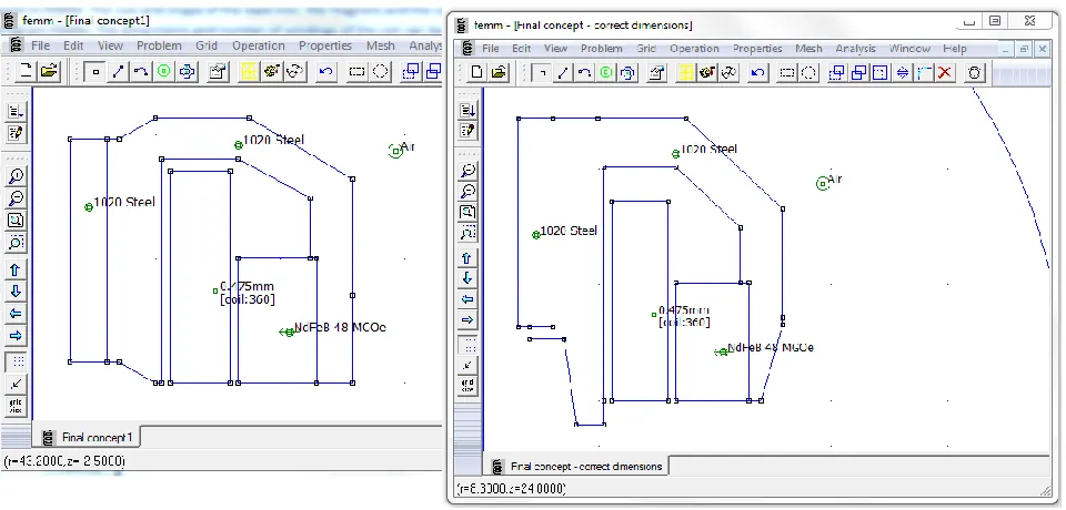
Figure 16: Design of the back iron, magnets and coil in FEMM (left: starting point, right: final design)

Putting the equation for the motor constant in the Matlab/Simulink model, together with the correct mass and resistance, will give the influence on the dissipated power and the therapy duration. The design fulfils the set requirements as shown in Figure 17.

The final design is based on the reduced values of the motor parameters and the therapy

parameters. The motor constant and the coil resistance have values of 80% and 76% of the original values respectively, and the stroke is set to 10mm. The therapy force range is reduced to 3N – 27N, and the therapy time is 96% of the original time. The therapy frequency range is not reduced.

y = -0.0004x3 _{- 0.0785x}2 _{+ 1.2152x +} 7.8268

0 2 4 6 8 10 12 14

0 5 10

M

o

to

r

co

n

stan

t

K

m

(

N

/A

)

27

Figure 17: a) dissipated power and b) therapy duration as function if therapy frequency and therapy force with reductions of functional design

5.3. Morphological diagram

There are other aspects that need to be designed next to the functional design. Two important sub problems are:

- Pretension is needed in the actuator to control the position.

- Linear guidance of the moving body to avoid forces and lost power in undesired directions.

Solutions for those sub problems are shown in a morphological diagram (Table 7 and Figure 18) and explained below. After designing this, concepts are assembled and the best concept is selected. Then some other connections between parts in the actuator can be designed.

Table 7: Morphological diagram in words

Function: Solution 1 Solution 2 Solution 3 Solution 4 Solution 5 Pretension Two custom

made

compression-extension springs (one on top, one at the bottom)

Two

compression springs (one on top, one at the bottom)

Parallel compression springs (multiple springs on top, multiple at the bottom)

Extension spring on top,

compression spring at the bottom

Two leaf springs (one op top, one at the bottom)

Linear

guidance Sliding contact linear motion bearing Rolling element linear motion bearing Elastic bearing

(leaf springs) Hydrostatic/aerostatic linear motion bearing

28

Function: Solution 1 Solution 2 Solution 3 Solution 4 Solution 5 Pretension

Linear guidance

Figure 18: Morphological diagram

5.3.1. Pretension

There are five mean solutions to create pretension in the actuator using springs. The advantages and disadvantages of these solutions are explained here. Also, some basic calculations are performed to see if the solution is feasible.

Solution 1: custom compression-extension springs

The dimensions for the compression-extension spring are calculated using the spring calculator as shown in Figure 19. But the desired deflection for the springs is only half of the total stroke for these springs since the equilibrium position of the spring is also the equilibrium position of the moving body. If the stroke is divided in two, the spring force is also half the size. This will give dimensions of the spring as shown in Table 8 where Lc is the length of the spring in compressed

state, and L0 the length of the spring in equilibrium position. This gives the dimensions for two

springs in parallel, one on top of the back iron and one at the bottom. Another option is putting more springs in parallel. The dimensions of the springs for six in parallel are also shown in Table 8.

Figure 19: Dimension calculator for springs [3]

Table 8: Dimensions of compression-extension spring

2 parallel (1 top, 1 bottom)

6 parallel (3 top, 3 bottom) Calculator Calculator

d (mm) 0.77 0.40

D (mm) 8.0 5

d=0.32*10^-3; %diameter of the wire (m)

D=3.2*10^-3; %mean diameter of the spring (m)

n=14; %number of active coil windings (-)

G=79.3*10^9; %shear modulus

F=2.54; %spring force (N)

Lc=n*d; %spring length compressed (m)

f=64*n*(D/2)^3*F/(d^4*G); %spring deflection (m)

k=F/f %spring stiffness (N/m)

L0=Lc+f; %spring length free/equilibrium (m)

29

n (-) 9 8

𝐹_𝑚𝑎𝑥 (N) 3.8 1.27 Lc (mm) 6.93 3.2

f (mm) 5.03 5.00

k (N/m) 756 254

σ (MPa) 169.6 253

L0 (mm) 11.96 8.2

Compression-extension springs need to be custom made since they are not found in a catalogue of suppliers. This is a disadvantage since it will increase the production costs for the springs.

Furthermore, these springs need to be attached between the stationary and moving body. This can be done by clamping with a linear shaft support block or with a wire robe clamp as shown in Figure 20. This is integrated with the back iron and assembled on top and on the bottom of the stationary body.

a) b)

Figure 20: Example of a) a linear shaft support block, b) wire robe clamp

Solution 2: Two compression springs

Compression springs are used instead of compression-extension springs. This will increase the deflection the spring should withstand to 10mm. An advantage is that compression springs are widely available in all kind of dimensions and stiffness.

Using some calculations and iteration, some dimensions for suitable springs are obtained using the spring calculator as shown in Figure 19, which also explained the used parameters. Two suitable springs are found in the catalogue of Amatec[4]_{, these are shown in Table 9. The same calculation}

can be done for two extension springs, this will give a spring with the same stiffness. But this sub concept is not mentioned any further since the effect is the same, but the assembly of extension springs is much more complicated than the assembly of compression springs.

Table 9: Dimensions springs solution 2 [4]

Configuration: 2 parallel (1 top, 1 bottom)

Name: Calculator D21842 C0480-035-1250 S

d (mm) 0.95 0.8 0.89

D (mm) 11.4 11.2 11.3

n (-) 7.2 4 5.2

𝐹_𝑚𝑎𝑥 (N) 7.6 11.83 17.38

Lc (mm) 6.84 6.77 10.85

f (mm) 10.04 16.23 20.90

k (N/m) 756.9 730 830

σ (MPa) 257 423 310

30

Solution 3: Parallel compression springs

Instead of using just one compression spring on the top and one at the bottom of the moving body, it is also possible to use multiple springs at both sides. The springs all work in parallel, so the total spring stiffness is the sum of the spring stiffness of all the springs. Also, the total spring force is the sum of the spring force of all the springs added. Using this, multiple weaker springs can be used to achieve the same total spring stiffness. The dimension calculator as shown in Figure 19 is used again to find possible solutions for parallel configurations. Again suitable springs are found in the catalogue of Amatec[4]_{. The results are shown in Table 10.}

Table 10: Dimensions springs solution 3 [4]

Configuration 6 parallel

(3 top, 3 bottom)

8 parallel

(4 top, 4 bottom)

12 parallel (6 top, 6 bottom) Name Calculator D20780 Calculator D20790 Calculator D20790

d (mm) 0.4 0.32 0.32 0.32 0.35 0.32

D (mm) 4 3.2 3.2 3.2 4 3.2

n (-) 16 14 16 20 20 20

Fmax (N) 2.54 3.16 1.905 3.16 1.27 3.16

Lc (mm) 6.4 4.48 5.12 8.9 7 8.9

f (mm) 10.25 11.21 9.6091 20.4 10.93 20.4

k (N/m) 250 230 198 160 0.12 160

σ (MPa) 404 632 474 316 302 316

L0 (mm) 16.65 15.69 14.73 29.3 17.93 29.3

Solution 4: One extension spring in combination with one compression spring

One extension spring is connected on the top side of the moving body, and one compression spring is connected at the bottom of the moving body. This will give another equilibrium position of the moving body. In rest, the moving body will be located at position 0, as far away from the patient as possible.

The influence of this change in rest position on the dissipated power is investigated before considering this concept further. Matlab/Simulink simulations give the average dissipated power for this sub concept. Different spring frequencies are used to see what the influence would be. The results are shown in Table 11. From these results, is can be concluded that the change in

equilibrium position will cause a higher dissipated power which is undesired.

Table 11: Average dissipated power

Spring frequency (Hz) Average 𝑷_{𝒅𝒊𝒔𝒔} (W) Original rest position (middle) 12.4 1.5299

New rest position (top) 10.0 1.9227

12.4 1.7972

15.0 2.0792

Solution 5: Leaf springs

31

springs is that the deflection in only half of the stroke: 5mm. Another advantage is that they fulfil the function of linear guidance as well.

A simple calculation of a leaf spring can be made by modelling it as a bending beam. This will give dimensions of the beam which give a rough impression about the sizes to see if it is a realistic solution. The calculations are shown in Figure 21. This gives dimensions of the leaf spring in the same order of magnitude as the actuator.

Figure 21: Dimension calculator of the leaf spring

5.3.2. Linear guidance

There are five mean solutions for linear guidance of the moving body in the actuator [5]_{. The}

advantages and disadvantages of these solutions are explained here. Also, some basic calculations are performed to see if the solution is feasible.

Solution 1: Sliding contact linear motion bearing

A sliding contact linear motion bearing is usually called a plain bearing. Advantages of this type of bearings are the low price, the bearings are very thin, and will be low weight. But plain bearings have one big disadvantage: the friction between the two bearing surfaces will cause wear and temperature rise of the bearing which will decrease the lifetime of the bearing and increase the dissipated power. The friction in a plain bearing is dependent on the sliding contact surface, the load, and the sliding velocity [6]_{. This application has a high sliding velocity and distance, so the life}

time of the sliding bearing will be too short.

Solution 2: Rolling element linear motion bearing

There are two types of linear rolling bearings: linear rails, and linear shaft bearings. Both types would be ball bearings. The preference would be the shaft bearing, since the rails are bigger and would add more weight to the actuator. The shaft bearing is located at the centre of the actuator where unused space is left.

Disadvantages of ball bearings are the friction which can cause wear, and the noise the bearing will produce while moving. An advantage is the accuracy of the linear guidance.

To determine if ball bearings have a long enough life time, some calculations are performed. As requirement from the customer, a lifetime of 1217 hours is needed (2 times 20 minutes a day, for 5 years). The method to calculate the life time of a bearing is described in [7]_, [8] _and [9]_{. This method is}

for rotation bearings. Some adjustments are made to calculate the lifetime for the linear bearing. These are described in [10] _and [11]_{. This gives an expression for the life time of a linear bearing in}

hours:

syms L b % Length L, width b of the material, m

F=7.6; % Spring force, N

k=1520; % Spring stiffness, N/m

sigma=400*10^6; % Average stress, Pa

E=210*10^9; % Elastic modulus, Pa

delta=0.005; % Deflection, m

h=0.5*10^-3; % Height of the material, m

32

𝐿10 = (833_𝐻∙𝑛) (𝐶_𝑃𝑟) 3

(8)

Here is 𝐻 the travelled distance per oscillation in meter, n is the number of oscillations per minute,

𝐶𝑟 the basic dynamic load rating, and 𝑃 the equivalent dynamic load rating.

Two small bearings are found [12] _{and the life time is calculated. These bearings are: L510X} [12] _and

one type that is slightly bigger: L612X [12]_{. The dimensions of the bearings are shown in Table 12.}

Some other properties of the bearings are needed for the calculation:

- 𝑍 = 10 (number of balls in a row) - 𝐹𝑟 = 𝑚𝑔 = 2.5 𝑁 (radial load)

- 𝐹𝑎= 30 𝑁 (axial load)

- 𝑛 = 1200 𝑜𝑠𝑐 (oscillations per minute) - 𝐻 = 0.020 𝑚 (distance per oscillation)

- 𝑃 = 𝑋𝐹𝑟+ 𝑌𝐹𝑎 (equivalent dynamic load rating, X and Y can be determined using the values above)

Using this and the method as described by Minebea [7] the lifetime for normal use for the L510X and the L612X bearings is calculated. This gave a lifetime of 791 hours and 3668 hours respectively. A life time of 1217 hours is needed in the actuator, so only the L612X bearing can be used for this application.

Table 12: dimensions of the bearings [12]

L510X L612X

dinside= 5 mm dinside= 6 mm

Doutside = 10 mm Doutside = 12 mm

Lbearing = 14 mm Lbearing = 18 mm

Øballs = 1.250 mm Øballs = 1.588 mm

Cr = 118 N Cr = 220 N

Solution 3: Elastic bearing

An elastic bearing would be a leaf spring. This can be applied in two ways. The first option is to make the leaf spring in such a way that it is just big and strong enough to fulfil the function of linear guidance. There is still another spring needed to cause the pretension. The second option is to design a leaf spring that causes the pretension, which automatically will cause linear guidance of the moving body.

The first type is based on designing and controlling degrees of freedom [13]_{. The actuator should}

33

𝐹_{𝑏𝑢𝑐𝑘𝑙𝑖𝑛𝑔}= 4𝜋2 𝐸𝐼

𝐿_𝑒2 (9)

With:

𝐼𝑠𝑞𝑢𝑎𝑟𝑒 𝑤𝑖𝑟𝑒 =₁₂1 𝑡4 (10)

𝐼_{𝑟𝑜𝑢𝑛𝑑 𝑤𝑖𝑟𝑒} =₆₄1 𝜋𝑑4 ₍₁₁₎

𝐿𝑒= 2𝐿 (12)

Using these equations, the combination of the length and thickness of the wire flexure can be

calculated. For a length 𝐿 = 30 𝑚𝑚, the thickness of a square wire flexure is 𝑡 = 0.336 𝑚𝑚 and for a round wire flexure it would be 𝑑 = 0.384 𝑚𝑚. This will give the wire flexure a spring constant of 24.849N/m and the total stiffness of the six wire flexures which account for the linear guidance will be 149.09N/m.

The wire flexures are tested for bucking with an applied force in axial direction. But a force in tangential direction should not cause movement and deflection in this direction, so the stiffness of the wire flexures in this direction is also calculated [14]_.

𝑘_𝑎= _𝐿 1

𝐸𝐴+ 𝑥2𝐿 700𝐸𝐼

(13)

𝑘_𝑡 =12𝐸𝐼

𝐿3 (14)

For a wire flexure of length 𝐿 = 30 𝑚𝑚, and a square cross section of thickness 𝑡 = 0.336 𝑚𝑚, this gives an axial stiffness of 165 kN/m, and a tangential stiffness of 25 N/m.

There are also two ways of connection the leaf springs to the statically body and the moving body which can be considered. This should be attached on two circles. The inner circle can be attached to the statically body or to the moving body, and the outer circle to the static body and the moving body respectively. The connection depends on the dimensions of the other components.

Solution 4: Hydrostatic/aerostatic linear motion bearing

34

Solution 5: Magnetic linear motion bearing

Linear guidance with magnetic linear motion bearings is not investigated any further because the magnetic field of the bearing can interfere with the magnetic field of the actuator. Furthermore, a magnetic bearing uses electrical energy, so more power is needed to accomplish the movement of the moving body which is undesired. A big advantage is that there is no contact between the parts so there will be no friction and noise.

5.3.3. Elimination

Based on the gathered information some solutions will not be suitable for this application. Reasons for this are the price, life time, dissipated power or the complexity.

There were five solutions for the pretension. After some calculations, only the fourth solution (one extension spring and one compression spring) is eliminated since this will cause an unnecessary increase in the dissipated power. The third solution (parallel springs) is also undesired since this is more complex to assemble than just two springs. But if there is a problem with the connection of one spring in a later stage of the design process, this would still be a possible alternative.

From the five solutions for the linear guidance, three solutions are eliminated. These are the sliding bearing, the hydrostatic bearing and the magnetic bearing because of high friction and short life time, price and complexity, and incompatibility respectively. Only rolling bearings and elastic bearing are considered in the further design steps.

5.4. Concepts

From the gathered information and suggested solutions, four concepts are composed which will be investigated in more detail.

- Concept 1: Use custom compression-extension springs in combination with a ball bearing. - Concept 2: Use compression springs in combination with a ball bearing.

- Concept 3: Use compression springs in combination with an elastic bearing.

- Concept 4: Use a membrane spring with the desired stiffness to fulfil the two functions of

pretension and linear guidance with one solution.

The concepts are designed in more detail and drawn in SolidWorks. Furthermore, aspects as the price, size, weight, aesthetics, and safety are investigated. Based on these aspects, the concepts will be ranked and a final concept can be made.

5.4.1. Concept 1: compression-extension springs with ball bearing

This concept with compression-extension springs is complicated to assemble if only one spring is used on the top of the moving body and one at the bottom of the moving body. The spring should be placed in the centre of the back iron, but the ball bearing is also located there. This can be solved in two ways:

- Use more parallel springs at both sides of the moving body. These springs can be located

off-centre which will give space for the bearing in the centre.

- Use a linear guidance bearing that is not located in the centre but at the outside of the

35

The second solution will still be complicated to make, so it is chosen to continue with the first option: use more parallel springs. This concept is shown in Figure 22. It is chosen to use three springs on top of the moving body and three at the bottom. The properties of the springs are estimated using the spring calculator and gives the dimensions as shown in Table 8. This gives an indication about the size of the springs. These springs need to be custom made.

The connection of the springs on the other components will be done with a linear shaft support block as shown in Figure 20a. The bearing that is used in the concept is from Micromo [12]_{, bearing}

code L612X. This bearing has the following dimensions: 𝑑𝑖𝑛𝑠𝑖𝑑𝑒 = 6𝑚𝑚, 𝐷𝑜𝑢𝑡𝑠𝑖𝑑𝑒 = 12𝑚𝑚,

𝐵 = 18𝑚𝑚, Ø_{𝑏𝑎𝑙𝑙𝑠}= 1.588𝑚𝑚, 𝐶_𝑟 = 220𝑁.

a) b)

Figure 22: SolidWorks sketch of concept 1, a) complete view, b) cross sectional view, ¾ of actuator. Red: magnets, green: back iron, yellow: bearing, brown: coil, blue: magnet retaining ring.

Advantages of this concept are:

- The springs are in relaxed position (not compressed and not extended) in the equilibrium

position of the moving body.

Disadvantages of this concept are:

- The actuator is complex to assemble. The springs are very small and need to be clamped in

the linear shaft support block which are also very small and include a lot of small screws. This will make the design complex and hard to assemble.

- Bearings make noise due to friction which might be very unpleasant for the user.

36 - The springs can be relocated and placed next to the back iron instead of on top and

underneath it. This will decrease the height of the actuator but increase the diameter of the actuator.

- The use of compression-extension springs allows it to use springs only at one side of the

moving body. This will cause a significant decrease in the height of the actuator and decrease the amount of components.

5.4.2. Concept 2: compression springs with ball bearing

Concept 2 is shown in Figure 23. The design has two parallel compression springs, one on top of the moving body, and one at the bottom. The compression springs that are used in this design are the D21842 springs, the properties are shown in Table 9.

The bearing that is used in the concept is the same as in concept 1, from Micromo [12]_{, bearing code}

L612X. This bearing has the following dimensions: 𝑑𝑖𝑛𝑠𝑖𝑑𝑒 = 6𝑚𝑚, 𝐷𝑜𝑢𝑡𝑠𝑖𝑑𝑒 = 12𝑚𝑚, 𝐵 = 18𝑚𝑚,

Ø_{𝑏𝑎𝑙𝑙𝑠}= 1.588𝑚𝑚, 𝐶_𝑟 = 220𝑁.

a) b)

Figure 23: SolidWorks sketch of concept 2, a) complete view, b) cross sectional view, ¾ of actuator. Red: magnets, green: back iron, yellow: bearing, brown: coil, blue: retaining rings.

Advantages of this concept are:

- The actuator is very compact and small.

- The concept has just a few additional components which are not complicated to assemble.

Disadvantages of this concept are:

37 5.4.3. Concept 3: compression springs with elastic bearing

This design has two parallel compression springs, one on top of the moving body, and one at the bottom as shown in Figure 24. The compression springs that are used in this design are the D21842 springs, just as in concept 2. The properties are shown in Table 9.

Wire flexures with a diameter of 0.44 mm and a length of 30 mm are used to ensure the linear guidance of the moving body. The spring constant of one wire flexure follows from buckling calculations and is equal to 𝑘 = 45𝑁/𝑚. So the total stiffness of the wire flexures is 𝑘 = 270𝑁/𝑚. The total stiffness the moving body experience is caused by the helix springs and the wire flexure which are all in parallel. This will give a total stiffness of: 𝑘_𝑡𝑜𝑡 = 2 ∙ 𝑘_{ℎ𝑒𝑙𝑖𝑥}+ 6 ∙ 𝑘_{𝑤𝑖𝑟𝑒}= 1730 𝑁/𝑚

which gives a spring frequency of 13.24 Hz.

For the wire flexure of length 𝐿 = 30 𝑚𝑚, and a square cross section of thickness 𝑡 = 0.44 𝑚𝑚, this gives an axial stiffness of 422 kN/m, and a tangential stiffness of 73 N/m.

a) b)

Figure 24: SolidWorks sketch of concept 3, a) complete view (without top), b) cross sectional view, ¾ of actuator. Red: magnets, green: back iron, brown: coil, blue: magnet retaining ring, orange/red: wire flexures.

Advantages of this concept are:

- Little noise.

- The actuator is small in height.

Disadvantages of this concept are:

- The wire flexures are very small and thin what will make it almost impossible to make and

to assemble. The wire flexures need to be clamped in the stationary body and screwed to the moving body. This will give a lot of small components and a lot of work to assemble.

- The wire flexures need to have a length of 30 mm to be able to withstand the radial force

and the stroke. This will give a design with a large diameter of the actuator.

38 - The wire flexures can be made with a square cross section and be bended to decrease the

diameter of the actuator.

5.4.4. Concept 4: membrane spring

This concept has six leaf springs, three on top and three at the bottom of the moving body as shown in Figure 25. The idea of this design is the same as the wire flexures, but those are made

bigger/wider to get the stiffness that is needed for the pretension. The composition of the leaf springs is the same as for the wire flexures which will give the same effect for the linear guidance. Leaf springs with a length of 44.4 mm, width of 6.7 mm, and a thickness of 0.5 mm are used.

a) b)

Figure 25: SolidWorks sketch of concept 4, a) complete view, b) cross sectional view, ¾ of actuator. Red: magnets and leaf springs, green: back iron, brown: coil, blue: magnet retaining ring.

Advantages of this concept are:

- The actuator is small in height.

- The concept has just a few components which are not complicated to assemble. - Little noise.

Disadvantages of this concept are:

- The leaf springs need to have a length of 44.4 mm to be able to withstand the radial force

and the stroke. This will give a design with a large diameter of the actuator.

In a later stadium of the design process, some possible improvements are:

- The design of the membrane spring is only based on the calculations of a leaf spring using

the deflection formulas. The design and the diameter of the membrane spring can be optimised to decrease the total diameter of the actuator.

- The radius of the inner circle of attachment of the leaf springs can be made smaller. Some