Discovering transcriptional modules by Bayesian data integration

(1)

University of Warwick institutional repository: http://go.warwick.ac.uk/wrap

This paper is made available online in accordance with

publisher policies. Please scroll down to view the document

itself. Please refer to the repository record for this item and our

policy information available from the repository home page for

further information.

To see the final version of this paper please visit the publisher’s website.

Access to the published version may require a subscription.

Author(s): Richard S. Savage , Zoubin Ghahramani , Jim E. Griffin,

Bernard J. de la Cruz and David L. Wild

Article Title: Discovering transcriptional modules by Bayesian data

integration

Year of publication: 2010

http://dx.doi.org/10.1093/bioinformatics/btq210

(2)

BIOINFORMATICS

Vol. 26 ISMB 2010, pages i158–i167doi:10.1093/bioinformatics/btq210

Discovering transcriptional modules by Bayesian data integration

Richard S. Savage

1 , Zoubin Ghahramani

2 , Jim E. Grifﬁn

3 , Bernard J. de la Cruz

4 and David L. Wild

1 ,

∗

1

_{Systems Biology Centre, University of Warwick, Coventry, CV4 7AL,}

2

_{Department of Engineering, University of}

Cambridge, Cambridge CB2 1PZ,

3

School of Mathematics, Statistics and Actuarial Science, University of Kent,

Canterbury, UK,

4

4035 Utah St, San Diego, CA 92104,USA

ABSTRACT

Motivation:We present a method for directly inferring transcriptional modules (TMs) by integrating gene expression and transcription factor binding (ChIP-chip) data. Our model extends a hierarchical Dirichlet process mixture model to allow data fusion on a gene-by-gene basis. This encodes the intuition that co-expression and co-regulation are not necessarily equivalent and hence we do not expect all genes to group similarly in both datasets. In particular, it allows us to identify the subset of genes that share the same structure of transcriptional modules in both datasets.

Results: We ﬁnd that by working on a gene-by-gene basis, our model is able to extract clusters with greater functional coherence than existing methods. By combining gene expression and transcription factor binding (ChIP-chip) data in this way, we are better able to determine the groups of genes that are most likely to represent underlying TMs.

Availability: If interested in the code for the work presented in this article, please contact the authors.

Contact:[email protected]

Supplementary information: Supplementary data are available at Bioinformaticsonline.

1 INTRODUCTION

Approaches to the elucidation of gene regulatory networks have

often relied on the use of clustering methodologies, grouping genes

on the basis of expression patterns over time, treatments and/or

tissues. The genes in a given cluster are usually assumed to be

potentially functionally related or to be influenced by common

upstream factors. For example, Eisen

et al.

(1998) found that in the

yeast

Saccharomyces cerevisiae

, genes that clustered together did

indeed often share similar biological function, and a large number

of subsequent authors have found the same, sometimes even being

able to verify the results experimentally (e.g. Ihmels

et al.

, 2002).

Application of these approaches to gene expression data have

led to the recognition that gene regulation is often performed by

regulatory programmes

or

transcriptional modules

(TMs); sets of

co-regulated genes that share a common biological function and are

regulated by a common set of transcription factors. Ihmels

et al.

(2002) devised a method for identifying TMs by assigning genes to

clusters in a context-dependent manner. A gene could be assigned

to several clusters, resulting in overlapping TMs, a feature which is

biologically meaningful since a gene could be involved in multiple

biological processes.

Clustering on the basis of expression data alone, however, only

indicates

co-expression

, and does not directly identify

co-regulation

.

∗_{To whom correspondence should be addressed.}

The expression patterns of genes in the same cluster may be

correlated for reasons other than co-regulation—the effects of

experimental measurement error may be important, for example.

Due to the complexity of gene regulatory networks, as well as

the limitations of any given source of noisy experimental data, it

is advantageous to make TM inferences using multiple sources of

data. In addition to gene expression data, a range of other data types

have been used to enhance the reconstruction of gene networks.

These include information about transcription factor binding derived

from experimental techniques such as ChIP-chip, sequence data and

even information derived from relevant scientific literature. Both

Segal

et al.

(2003a) and Kundaje

et al.

(2005) have described

methods to integrate expression and sequence data within the

framework of a probabilistic graphical model, using the method

of expectation maximization —a statistical technique for maximum

likelihood estimation of model parameters from incomplete data.

Segal

et al.

(2003b) applied a variant of this approach to infer

regulatory modules in

S.cerevisiae

, together with their component

regulators, under the assumption that the regulators themselves are

transcriptionally regulated, at least under a subset of conditions.

Bar-Joseph

et al.

(2003) described a method to integrate ChIP-chip and

expression data based on an exhaustive iterative search over possible

combinations of regulators, which identifies a subset of gene targets

with highly correlated expression patterns.

Dirichlet process mixture models (DPMs; Antoniak, 1974;

Ferguson, 1973) are a class of Bayesian non-parametric models that

has been widely used for clustering (Dahl, 2006; Liu

et al.

, 2006;

Medvedovic and Sivaganesan, 2002; Medvedovic

et al.

, 2004; Qin,

2006; Rasmussen

et al.

, 2009; Rasmussen, 2000; Wild

et al.

, 2002).

DPMs have the interesting property that the prior probability of

a new data point joining a cluster is proportional to the number

of points already in that cluster, thus encoding a natural clustering

tendency. Clustering strength is controlled via a hyperparameter

α

,

which sets the expected number of clusters as a function of the

number of clustered items. By inferring

α

we can therefore determine

the posterior distribution of the number of clusters.

Hierarchical Dirichlet Process models [HDPMs as defined by Teh

et al.

(2006)] are the hierarchical extension of DPMs. They consist

of a DPM for each of a number of different

contexts

, with the

mixture components for each context being drawn from a master

list of mixtures from the next level of the hierarchy. A wider range

of HDPMs are reviewed in Teh and Jordan (2010). Reid

et al.

(2009) use a type of HDPM to identify TMs from transcription

factor binding site sequence data. Gerber

et al.

(2007) use HDPMs

to model gene expression programs in a variety of tissues.

Effective combination of different datasets can be an effective

way to identify TMs. Liu

et al.

(2007) introduced a HDPM that

assigns a DPM to each of a pair of datasets (e.g. gene expression

(3)

and ChIP-chip) and connects them via a common hyperparameter,

α

.

By producing combined results from the sampled clustering for both

contexts, they are able to produce a form of flexible data integration.

As we shall see below, the Liu

et al

. approach is a special case of

the model we present in this article.

2 METHODS

Our aim is to cluster genes together on the basis of both gene expression and ChIP-chip (transcription factor binding site) information. We wish to identify the genes that possess the same clustering structure across both datasets, as these are more likely to represent underlying TMs and hence share specific biological function/s. We expect that the information coming from each dataset will be uncertain and possibly contradictory. Therefore, we wish to distinguish (on a gene-by-gene basis) between genes that can sensibly have their data fused and those for which there is contradiction.

2.1 The model

We construct our model (shown in Fig. 1) from a two-level hierarchy of DPMs. This model can be regarded as a modified version of the HDPM presented in Tehet al.(2006). A naïve use of HDPMs for data integration may fail since it assumes that all data sources are clustered identically. Our principal innovation is to include, for each gene, an indicator variable that determines whether the gene should join a cluster based on both data sources combined (via a product of likelihoods) or whether it should be clustered separately for each dataset.

The genes are assigned to three contexts, each defining a clustering partition via a DPM. One context contains the genes that are fused across the two datasets. The other two contexts are for the unfused genes, one clustering solely on the basis of expression data and the other using the transcription factor binding dataset. The fusion indicator variables are learnt as part of the inference process (carried out via a Gibbs sampler), allowing us to determine the posterior probability that any given gene will be fused.

We define our model as follows [using the same notation as Teh

et al. (2006)]. We haven genes, for each of which we have two sets of measurements (expression and ChIP-chip). Each gene can either be considered for the two datasets separately or we canfusethem together, giving a single (product) likelihood. This gives us three contexts overall. Let

xjibe the observed response fori-th gene in thej-th context. Note that when sampling, genes can flip from a fused to unfused state and vice versa.

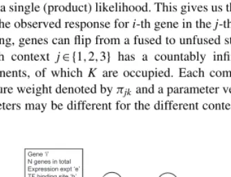
[image:3.728.100.267.557.685.2]

Each context j∈{1,2,3} has a countably infinite number of mixture components, of whichK are occupied. Each componentk∈{1,...,K}has a mixture weight denoted byπjkand a parameter vectorθjk, where the set of parameters may be different for the different contexts.

Fig. 1. Graphical representation of the model presented in this article. The parameters are defined in Section 2.

Each gene is assigned to a mixture component via the indicator variable

Zij, giving us the following equations.

P(Zij=k|π)=πjk (1)

The conditional likelihood for each gene is then:

P(xji|Zij=k,θ)=Lj(xji|θjk) (2)

where Lj is the likelihood we assign to model the data andθjk are the parameter values for mixture componentkin contextj.

These are assigned the stick-breaking prior associated with the Dirichlet process (Tehet al., 2006)

πjk=Vjk

i<k

(1−Vji) (3)

where Vjk are mutually independent and Vjk∼Be(1,α) which we write Stick(α). Marginalizing over the mixture weights gives us a DPM for each context. Similarly,are the mixture weights for the second level of the Dirichlet process hierarchy. Again, these are assigned a stick-breaking prior and marginalized over, so that they do not have to be considered explicitly in the analysis.

π|α0∼Stick(α0) (4)

|γ∼Stick(γ) (5)

The hyperparametersα0andγare the concentration parameters for the

two levels of the Dirichlet process hierarchy.α0 is shared across all three

contexts, representing the prior belief that they are all representing the same biological system and hence we should expect the same number of underlying TMs. These can be inferred and therefore are assigned vague gamma priors as follows.

α0∼Gamma(2,4) (6)

γ∼Gamma(2,4) (7)

We choose the component likelihoods to reflect the nature of the two datasets. For the expression data, we discretize the measured value for each gene into three levels, representing under-, over- or unchanged expression. This is something of a simplifying assumption, but makes our analysis more robust to the non-Gaussian noise typical of gene expression data, and is an approach that has been shown to be effective (see e.g. Gerberet al., 2007; Savageet al., 2009). We therefore choose the component likelihood for the expression data to be a naïve Bayes model, constructed from a product of multinomial distributions.

For the ChIP-chip data, we have statistical (P-value) information as to whether or not a given transcription factor binds to a given gene. By thresholding these values, we obtain sparse binary data, indicating whether binding has occurred. We choose to model these data using a so-called ‘bag-of-words’ model, e.g. a multinomial likelihood over transcription factors. This has the advantage that only counts over genes are important, meaning that a large number of zeros in the data can be handled safely. Note that in both cases we choose to apply (conjugate) Dirichlet priors.

For the expression data, we have

L1(x)=

a

(Ba)

(Na+Ba)

b

(xab+βab)

(βab) (8)

where Ba=bβab and Na=bxab,ais the index over features andb is the index over discrete data values. The βab are the Dirchlet prior hyperparameters, which in this case are all set to 0.5 (the Jeffreys’ value).

For the ChIP-chip data, we have

L2(x)=

(B)

(N+B)

a

(xa+βa)

(βa) (9)

(4)

R.S.Savage et al.

(the Jeffreys’ value). The above two equations are obtained from Equation (2) for a particular clusterkby integrating out the parametersθ.

We encode the notion of data fusion for a given geneiby allowing the possibility of taking the product of likelihoods over the two datasets. So, if the likelihood parameters for contexts one and two are given byθ1iandθ2i, we have the following equations.

We introduce an extra latent variablerifor each gene with

P(ri=1)=w, P(ri=0)=1−w. (10)

Ifri=1 (corresponding to a fused gene) then:

θi=(θ1iθ2i)∼F3 (11)

And ifri=0 (corresponding to an unfused gene) then:

θ1i∼F1 (12)

θ2i∼F2 (13)

This defines three contexts. Unlike the HDPM, we have

F1∼DP(α0,F0(1)) (14)

F2∼DP(α0,F0(2)) (15)

F3∼DP(α0,F0) (16)

F0(θ1,θ2)∼DP(γ,H) (17)

where F₀(j) represents the marginal distribution of θj under F0. The

hierarchical Dirichlet process structure allows sharing of clusters across the unfused and fused contexts. For example, an unfused gene can be allocated to the same cluster as fused genes for gene expression but allocated to a different cluster (shared by different fused genes) for transcription factors.

We choose to fixw=0.5 for the analyses in this article, representing that we have no prior knowledge of the degree to which these datasets should fuse. We note that it is also straightforward to sample fromwand we run a test of this, the results of which can be seen in Table 3. Details of the algorithm to implement this model, in particular a Gibbs sampler, can be found in Appendix A.

2.2 Special cases of the model

Our model has two special cases that are of interest and represent alternative ways of approaching data integration.w=0 gives us the model of Liuet al.

(2007). In this model, there is no direct data fusion (in the sense that all theri=0). Instead, information is shared via a common hyperparameter,α0,

between the clustering for each dataset. Each dataset is therefore clustered (almost) separately, but benefiting from this weak sharing of information via the hyperparameter.w=1 gives us simple data integration by taking the product of likelihoods and forcing all genes to be part of a single clustering partition. Withw=1, only the fused context is used (genes can never be unfused) and so we have a straightforward DPM with a product of likelihoods over the two datasets.

2.3 Extracting modules from the posterior samples

Once we have explored the model space using Markov chain Monte Carlo (MCMC) sampling, we wish to extract useful results from the samples. In particular, we wish to identify TMs, which in our model correspond to groups of genes that fused with high probability and that are often found in the same fused cluster. This is a non-trivial challenge, as each MCMC sample contains a large number of parameters (mixture component labels for each gene in each of three contexts,rifor each gene, plus the global hyperparameters). We therefore require a way to summarize the results. To do this, we choose to form a posterior similarity matrix (Fritsch and Ickstadt, 2009). From this we will extract a clustering partition, which will correspond to transcriptional modules. The posterior similarity matrix is an (ngenes×ngenes) matrix where each element gives the posterior probability

that a given pair of genes are found in the same cluster (and hence also in the same context). These values can be estimated simply by counting the MCMC samples in the appropriate way.

A major advantage of our model is that it identifies how likely each gene is to be fused (estimated from therivalues over MCMC samples). By rejecting genes with lowP(ri=1|x), we can identify more tightly defined TMs. For this article, we choose to define ‘fused’ as beingP(ri=1|x)≥0.5 (the prior value we assign towfor the full model).

From the posterior similarity matrix, we extract the most likely cluster partition using the method of Fritsch and Ickstadt (2009), which minimizes a defined loss function that is equivalent to maximizing the adjusted Rand index between estimated and true clustering partitions. We note that this represents a summarization of the full results implicit in the analysis. Some kind of compromise of this nature is inevitable, simply due to the richness of the posterior distribution of our model. As we shall demonstrate, this approach still leads to superior results and hence biological insight.

We can also extract other useful quantities from the posterior MCMC samples. For example, the 1D marginal distributions of the hyperparameters, the number of fused clusters and the number of fused genes are all easily determined.

2.4 Quality measures

We are interested in identifying TMs with well-defined biological function/s. Our quality measures should therefore reflect this. We choose two measures, both using the Gene Ontology (GO) database.

The first measure is theBiological Homogeneity Index(BHI; Datta and Datta, 2006). This is a global measure of how biologically homogeneous a given clustering partition is (as measured here using GO annotations). Clusters where many genes share annotations will lead to a high BHI score and vice versa. Perfect agreement for all GO terms (which is highly unlikely) would lead to a score of unity.

We compute error estimates of these BHI scores by performing 10 random combinations of the 20 MCMC chains (chosen via bootstrap sampling, eg. so that a given chain may be selected multiple times), finding in each case the clustering partition and hence the BHI score. This gives us a measure of any uncertainty due to inadequate mixing of the MCMC chains.

The second measure is to find GO terms that are over-represented in any given module, relative to the background population of genes. We use the R package GOstats (Falcon and Gentleman, 2007) to apply a hypergeometric test to each GO term in each cluster. We apply this analysis to all GO terms in the three ontologies (cellular component, molecular function and biological process). We account for the dependent, hierarchical structure of the ontologies using the relevant option in the call to the GOstats function ‘hyperGTest’. We correct for multiple hypotheses using a Bonferroni correction.

2.5 Data

We perform two different analyses in this article, in each case analysing data fromS.cerevisiae. To facilitate comparison with earlier work, in both cases we use ChIP-chip data from Leeet al.(2002) to provide information on transcription factor binding activity. This dataset contains nearly 4000 interactions between regulators and promoter regions, representing 6270 yeast genes and 106 transcriptional regulators.1

We use two different gene expression datasets in the two analyses. The first one (referred to subsequently as thegalactose utilizationdata) is taken from a subset of the expression dataset of Idekeret al.(2001), which has been widely used for the validation of clustering methods (Savageet al., 2009; Yaoet al., 2008; Yeunget al., 2003). These data are a series of expression

1_{A more extensive set of ChIP-chip data from the same laboratory was later}

published by Harbisonet al.(2004). This use of this dataset in place of that of Leeet al.(2002) does not materially change the conclusions of this article, as illustrated in Table 3.

(5)

measurements across 20 experiments representing systematic perturbations of the yeast galactose utilization pathway. The subset used consists of 205 genes whose expression patterns reflect four functional categories (biosynthesis, protein metabolism and modification; energy pathways, carbohydrate metabolism and catabolism; nucleobase, nucleoside, nucleotide and nucleic acid metabolism; transport), based on GO annotations. However, as Yeunget al.(2003) note, since this array data may not fully reflect these functional categories, these classifications should be used with caution.

For the other analysis (referred to as thecell cycle data), we use gene expression measurements of the mitotic yeast cell cycle of Choet al.(1998), which was chosen to facilitate direct comparison with the results of Liuet al.

(2007), who also analysed this data. For this dataset, we keep only the genes that were identified as having a Kyoto Encyclopedia of Genes and Genomes (KEGG) pathway, following the procedure of Liuet al.(2007). We note that there are small differences in the number of genes selected in this way (949 versus 1165 in this article), due to differences in the version of the KEGG database used.

2.6 Data processing

For both expression datasets, we discretize the data into three levels. This has two benefits. First, it makes our analysis more robust to the non-Gaussian (and hence hard to model) noise distribution of the data. Secondly, it makes the task of data modelling more straightforward. To optimize the binning of the data, we use the Bayesian Hierarchical Clustering (BHC) package (Savageet al., 2009) to find an optimized binning and assume that this will then also be reasonably optimal for this analysis.

For the ChIP-chip dataset, we follow the procedure of Leeet al.(2002) and threshold the data at aP-value of 0.001, giving us a sparse dataset where the detections are robust, at the expense of a larger proportion of false negatives (Leeet al. estimate 6–10% false positives and that about one-third of the interactions are missed).

3 RESULTS

The results of each data integration analysis are rich and detailed.

In this section, we consider a number of metrics and highlight

significant aspects of the results for each dataset. For comparison,

we also run clustering analyses using the BHC algorithm (Savage

et al.

, 2009) to analyse the gene expression data alone. This gives us

a baseline result with which to compare the data integration results.

It is important to assess the convergence of any MCMC analysis.

All analyses on the galactose dataset comprise 20 MCMC chains,

each of 50 000 samples (after removal of 10 000 burn-in samples).

All analyses on the cell cycle data set comprise 20 MCMC chains,

each of 5000 samples (after removal of 1000 burn-in samples). To

speed up our subsequent analyses, we sparse sample each chain by

a factor of 10.

We

include

as

Supplementary

Material

plots

of

1D

hyperparameter posterior PDFs, both overall and for each

MCMC chain. These demonstrate that the MCMC analyses are

converging adequately. We also perform Geweke convergence tests

(Geweke, 1992) on the hyperparameters of each chain (

α

0

and

γ

)

for the

w

=

0 .

5 case. For the galactose dataset, we find 30 of 40 tests

(20 chains, 2 hyperparameters) have a

z

-score

<

2, with a maximum

outlier of 3

.

48. For the cell cycle dataset, we find 28 of 40 tests

have a

z

-score

<

2, with a maximum outlier of 5

.

53. We conclude

that our chains are reasonably well (although not perfectly) mixed,

although in both cases it is important that we combine multiple

chains.

The algorithm is implemented in Matlab and run on 3 GHz cluster

nodes (20 in parallel, one per MCMC chain). On the galactose

utilization dataset (205 genes), the code produces 500 samples per

chain per hour. On the cell cycle dataset (1165 genes), the code

produces 40 samples per chain per hour. On a larger sample of

2332 genes [from the stress data of Gasch

et al.

(2000)], the code

produces 10 samples per chain per hour. This scaling suggests that

for large (genome-scale) datasets it may be of value to investigate

(for example) fast variational methods as an alternative to MCMC.

3.1 Galactose utilization dataset

In Table 1, we give the BHI scores for different analyses of the

galactose utilization dataset. The outcome from our model (fused

genes and

w

=

0 .

5) extracts a subset of 51 genes with an overall

BHI score that is 9% (3 SDs) higher than for any other method,

indicating a greater degree of biological functional coherence. We

note that all methods are superior to the BHC result for expression

data alone (BHI = 0.323), except for the ChIP only analyses.

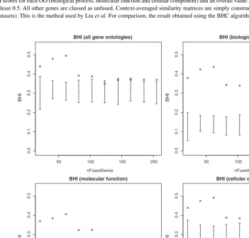
Figure 2 shows the variation of the BHI with the clustering

partition resulting from keeping the top

n

genes, as sorted by

P

(

r

i

=

1 |

x

). There is a clear enriching effect on the BHI (and hence

biological homogeneity) by selecting a subset of genes in this way.

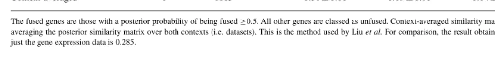
In Figure 3, we show a matrix of the significantly over-represented

GO terms in each of the clusters we extract for the model (fused

genes and

w

=

0 .

5). Notable are the density of hits, and also the

distinct block structure, which reflects that each cluster is tending

to capture all the significance for given GO terms. These GO

terms reflect the four functional categories previously identified

in this data, but detailed inspection of the functional annotations

of the genes in each cluster reveals a finer level of biological

specificity than previously identified. Cluster 1 (counted from

the left) comprises four genes involved in glycolysis and the

tricarboxylic acid (TCA) cycle. Cluster 2 represents genes involved

in replication and RNA processing, while Cluster 3 comprises

primarily ribosomal components. Cluster 4 comprises four hexose

transporters, including at least one pseudogene, which, despite being

non-functional, is nevertheless expressed.

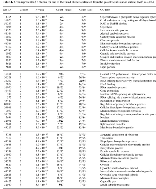
Table 4 shows comparisons of over-represented GO terms with

those obtained from the Liu method. In general, the data fusion

GO terms are more enriched, with lower

P

-values and, in almost

all cases, a higher proportion of the genes being annotated with

the term.

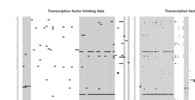
In Figure 4, we show the ChIP-chip data for the fused genes,

sorted by cluster membership. The structure in this plot (horizontally

aligned hits) shows certain transcription factors are contributing to

the data integration and, like Segal

et al.

(2003b), we find that

TMs are characterized by partly overlapping but distinct motif

combinations.

Table 3 shows some comparison analyses carried out using the

Harbison

et al

. (2004) ChIP data in place of that of Lee

et al

.

While the Harbison

et al

. data analysis finds more fused genes

(72 versus 51), the BHI scores are comparable. We also run an

analysis where we sample over

w

; in this case, the BHI scores are

marginally worse and there are fewer fused genes (56) than for the

w

=

0 .

5 case.

3.2 Cell cycle dataset

(6)

[image:6.728.50.553.87.208.2]

Table 1. The BHI scores for the galactose utilization dataset

Similarity matrix w No. of genes BHI (all) BHI (bp) BHI (mf) BHI (cc)

Fused genes 0.5 51 0.49±0.03 0.43±0.05 0.40±0.04 0.49±0.03

Fused genes 1 205 0.37±0.01 0.22±0.01 0.19±0.01 0.37±0.01

Unfused (expression only) 0 205 0.38±0.01 0.26±0.02 0.22±0.02 0.38±0.01

Unfused (expression only) 0.5 154 0.37±0.03 0.30±0.02 0.23±0.02 0.37±0.03

Unfused (ChIP chip only) 0 205 0.28±0.03 0.13±0.01 0.11±0.02 0.25±0.03

Unfused (ChIP chip only) 0.5 154 0.20±0.06 0.06±0.03 0.07±0.04 0.19±0.07

Context-averaged (Liuet al.) 0 205 0.38±0.01 0.26±0.02 0.22±0.01 0.38±0.01

Context-averaged 0.5 205 0.40±0.01 0.24±0.01 0.20±0.01 0.40±0.02

Context-averaged 1 205 0.37±0.01 0.22±0.01 0.19±0.01 0.37±0.01

We compute the BHI scores for each GO (biological process, molecular function and cellular component) and an overall value. The fused genes are those with a posterior probability of being fused of at least 0.5. All other genes are classed as unfused. Context-averaged similarity matrices are simply constructed by averaging the posterior similarity matrix over both contexts (i.e. datasets). This is the method used by Liuet al.For comparison, the result obtained using the BHC algorithm on the gene expression data alone is 0.323.

50 100 150 200

0.0

0.1

0.2

0.3

0.4

0.5

BHI (all gene ontologies)

nFusedGenes

BHI

50 100 150 200

0.0

0.1

0.2

0.3

0.4

0.5

BHI (biological processes)

nFusedGenes

BHI

50 100 150 200

0.0

0

.1

0.2

0.3

0.4

0.5

BHI (molecular function)

nFusedGenes

BHI

50 100 150 200

0.0

0

.1

0.2

0

.3

0.4

0.5

BHI (cellular component)

nFusedGenes

BHI

Fig. 2.Plots of the BHI for the galactose dataset, showing the variation with different numbers of fused genes. Shown are the BHI results for each GO separately, plus all three combined. In all cases, selecting 100 or fewer genes leads to an increase in the BHI score. The error bars show a distribution of randomized BHI scores where the cluster sizes and number of clusters are kept the same but gene names are drawn randomly from the 205 genes in the galactose dataset. By comparison, this gives us a measure of the enrichment of the fused gene clusters.

provides a slightly lower BHI score. In all cases, the data integration

provides benefit over simply using gene expression data and the

BHC algorithm (BHI = 0.285).

In the Supplementary Material we show the posterior similarity

matrix, sorted by cluster membership. The block-diagonal structure

shows the core of each cluster clearly defined. In this figure,

off-diagonal blocks may indicate one of two possibilities; it may

mean that there is

uncertainty

in whether a set of genes should

be assigned to one of the two clusters, or it may indicate a set

of genes that should really belong

simultaneously

to two clusters.

[image:6.728.125.477.258.593.2]

(7)

[image:7.728.138.490.62.222.2] [image:7.728.63.569.285.406.2]

Fig. 3. Graphical representation of the significantly over-represented GO terms for each cluster of genes, for the galactose utilization (left) and cell cycle (right) datasets. Black indicates that a given gene is annotated with the relevant GO term and that the term is over-represented in that cluster.

Table 2. The BHI scores for the cell cycle dataset

Fused genes 0.5 266 0.33±0.01 0.18±0.02 0.17±0.01 0.23±0.01

Fused genes 1 1165 0.30±0.01 0.09±0.01 0.14±0.01 0.20±0.01

Unfused (expression only) 0 1165 0.28±0.01 0.07±0.01 0.14±0.01 0.19±0.01

Unfused (expression only) 0.5 898 0.31±0.01 0.08±0.01 0.16±0.01 0.20±0.01

Unfused (ChIP chip only) 0 1165 0.30±0.01 0.05±0.01 0.12±0.02 0.24±0.02

Unfused (ChIP chip only) 0.5 898 0.25±0.03 0.06±0.01 0.13±0.03 0.21±0.02

Context-averaged (Liuet al.) 0 1165 0.29±0.01 0.09±0.01 0.14±0.01 0.20±0.01

Context-averaged 0.5 1165 0.30±0.01 0.08±0.01 0.15±0.01 0.20±0.01

Context-averaged 1 1165 0.30±0.01 0.09±0.01 0.14±0.01 0.20±0.01

The fused genes are those with a posterior probability of being fused≥0.5. All other genes are classed as unfused. Context-averaged similarity matrices are simply constructed by averaging the posterior similarity matrix over both contexts (i.e. datasets). This is the method used by Liuet al.For comparison, the result obtained using the BHC algorithm on just the gene expression data is 0.285.

Table 3. The BHI scores for galactose utilization with Harbisonet al.ChIP data, for comparison with Table 1

fused genes 0.5 72 0.49±0.01 0.42±0.01 0.35±0.01 0.49±0.01

fused genes 1 205 0.39±0.01 0.22±0.01 0.19±0.01 0.37±0.01

fused genes sampled 56 0.49±0.01 0.40±0.01 0.32±0.01 0.49±0.01

The Leeet al. ChIP data are used in this article to mimick the Liuet al. analysis. The results here show that the Harbisonet al.data result in a greater number of fused genes, with similar overall BHI scores. Also shown are results for a run wherewis sampled using a Gibbs sampler. This shows a small degradation over thew=0.5.case.

The two clusters in question (Clusters 3 and 4, counted from the

left) do indeed share common GO annotations indicating metabolic

function (Fig. 3). Cell cycle regulation is a complex interplay of

many different external signals and intrinsic cell states (Bähler,

2005). The cell cycle is composed of at least four phases: S, synthesis

phase wherein DNA is being replicated; G1, gap 1; M, mitosis

where the yeast cell physically pulls chromosomes into the daughters

and then separates; and G2, gap 2. The transitions between phases

are critical checkpoints. There cell division is blocked by various

conditions; for example, signals indicating there is DNA damage

or incomplete DNA replication will block cells from going from

S

→

G1. Thus, it would be expected that there may be multiple

regulatory pathways, some of which likely overlap.

In Figure 3, we show a matrix of the significantly over-represented

GO terms in each of the clusters we extract. As with the galactose

utilization dataset, there is good block structure, although in this

larger dataset there are some high-level GO terms that are significant

in more than one cluster.

[image:7.728.63.565.473.533.2]

(8)

[image:8.728.48.553.83.695.2]

Table 4. Over-represented GO terms for one of the fused clusters extracted from the galactose utilization dataset (withw=0.5)

GO ID Cluster P-value Count (fused) Count (Liu) GO term

4365 1 9.8×10−6 _2/4 ₃_/₉ _{Glyceraldehyde-3-phosphate dehydrogenase (phosphorylating) activity}

16620 1 5_.0_×10−4 _2/4 ₃_/₉ _{Oxidoreductase activity, acting on aldehyde/oxo donors, NAD/NADP acceptor}

51287 1 1.1×10−3 _2/4 ₃_/₉ _{NAD or NADH binding}

6096 1 3.6×10−8 ₄_/₄ ₉_/₉ _Glycolysis

19320 1 3.3×10−7 ₄_/₄ ₉_/₉ _{Hexose catabolic process}

46164 1 7.4×10−7 ₄_/₄ ₉_/₉ _{Alcohol catabolic process}

16052 1 3_.3_×10−6 ₄_/₄ ₉_/₉ _{Carbohydrate catabolic process}

6094 1 1.9×10−5 ₃_/₄ ₇_/₉ _{Gluconeogenesis}

46364 1 1.2×10−4 3/4 7/9 Monosaccharide biosynthetic process

19752 1 5.7×10−4 ₄_/₄ ₈_/₉ _{Carboxylic acid metabolic process}

42180 1 6.4×10−4 ₄_/₄ ₈_/₉ _{Cellular ketone metabolic process}

6082 1 6.8×10−4 4/4 8/9 Organic acid metabolic process

6800 1 1.2×10−3 _2/4 ₃_/₉ _{Oxygen and reactive oxygen species metabolic process}

1950 1 1.7×10−4 ₃_/₄ ₇_/₉ _{Plasma membrane enriched fraction}

5626 1 2.1×10−3 3/4 7/9 Insoluble fraction

5811 1 3.3×10−3 _2/4 ₃_/₉ _{Lipid particle}

16251 2 8_.9_×10−5 _5/23 ₇_/₈₄ _{General RNA polymerase II transcription factor activity}

30528 2 1.6×10−3 ₆_/₂₃ ₂₆_/₈₄ _{Transcription regulator activity}

31202 2 1.6×10−3 ₄_/₂₃ _22/84 _{RNA splicing factor activity, transesterification mechanism}

3677 2 6_.1_×10−3 _6/23 ₁₄_/₈₄ _{DNA binding}

16070 2 9.2×10−12 ₁₉_/₂₃ ₅₃_/₈₄ _{RNA metabolic process}

10467 2 1.1×10−7 22/23 78/84 Gene expression

398 2 1.5×10−4 ₆_/₂₃ ₂₄_/₈₄ _{Nuclear mRNA splicing via spliceosome}

375 2 2.3×10−4 ₆_/₂₃ ₂₆_/₈₄ _{RNA splicing, via transesterification reactions}

45449 2 4.1×10−4 6/23 29/84 Regulation of transcription

80090 2 7.5×10−4 ₁₃_/₂₃ ₄₀_/₈₄ _{Regulation of primary metabolic process}

34961 2 1.2×10−3 ₁₇_/₂₃ ₅₂_/₈₄ _{Cellular biopolymer biosynthetic process}

9059 2 2_.9_×10−3 ₁₇_/₂₃ ₅₂_/₈₄ _{Macromolecule biosynthetic process}

51171 2 6.1×10−3 ₈_/₂₃ ₃₁_/₈₄ _{Regulation of nitrogen compound metabolic process}

5634 2 2.6×10−8 _22/23 ₁₅_/₈₄ _Nucleus

32991 2 7_.9_×10−5 _18/23 ₂₄_/₈₄ _{Macromolecular complex}

5681 2 1.3×10−4 ₅_/₂₃ ₁₉_/₈₄ _{Spliceosomal complex}

43227 2 3.9×10−4 23/23 83/84 Membrane-bounded organelle

3735 3 1.3×10−21 ₁₆_/₁₇ ₇₅_/₇₅ _{Structural constituent of ribosome}

6412 3 3.4×10−10 13/17 49/75 Translation

43284 3 4.4×10−8 ₁₇_/₁₇ ₇₅_/₇₅ _{Biopolymer biosynthetic process}

34645 3 1.2×10−7 ₁₇_/₁₇ ₇₅_/₇₅ _{Cellular macromolecule biosynthetic process}

9058 3 4_.2_×10−6 _17/17 ₄₉_/₇₅ _{Biosynthetic process}

19538 3 7.2×10−6 ₁₃_/₁₇ ₄₉_/₇₅ _{Protein metabolic process}

34960 3 4.8×10−4 ₁₇_/₁₇ ₇₅_/₇₅ _{Cellular biopolymer metabolic process}

43170 3 9_.4_×10−4 ₁₇_/₁₇ ₇₅_/₇₅ _{Macromolecule metabolic process}

33279 3 3.7×10−21 ₁₆_/₁₇ ₇₅_/₇₅ _{Ribosomal subunit}

5829 3 1.1×10−13 ₁₆_/₁₇ ₇₄_/₇₅ _Cytosol

22627 3 3_.2_×10−11 ₈_/₁₇ ₃₃_/₇₅ _{Cytosolic small ribosomal subunit}

43232 3 8.3×10−10 ₁₆_/₁₇ ₇₅_/₇₅ _{Intracellular non-membrane-bounded organelle}

22625 3 1.1×10−9 ₈_/₁₇ ₄₁_/₇₅ _{Cytosolic large ribosomal subunit}

32991 3 1_.5_×10−6 ₁₆_/₁₇ ₇₅_/₇₅ _{Macromolecular complex}

44422 3 1.1×10−4 ₁₆_/₁₇ ₇₅_/₇₅ _{Organelle part}

32040 3 5.4×10−3 3/17 7/75 Small-subunit processome

51119 4 2.8×10−9 ₄_/₄ ₁₁_/₁₂ _{Sugar transmembrane transporter activity}

5353 4 3.2×10−7 3/4 10/12 Fructose transmembrane transporter activity

15578 4 3.2×10−7 ₃_/₄ ₁₀_/₁₂ _{Mannose transmembrane transporter activity}

5355 4 4.6×10−7 3/4 10/12 Glucose transmembrane transporter activity

22891 4 3.3×10−5 ₄_/₄ ₁₂_/₁₂ _{Substrate-specific transmembrane transporter activity}

5215 4 1.2×10−4 ₄_/₄ ₁₂_/₁₂ _{Transporter activity}

8645 4 1_.2_×10−9 ₄_/₄ ₉_/₁₂ _{Hexose transport}

8643 4 9.7×10−9 ₄_/₄ ₁₁_/₁₂ _{Carbohydrate transport}

55085 4 1.4×10−5 4/4 12/12 Transmembrane transport

51234 4 8.3×10−3 ₄_/₄ ₁₂_/₁₂ _{Establishment of localization}

5886 4 5.0×10−3 ₃_/₄ ₁₁_/₁₂ _{Plasma membrane}

Also shown is a comparison with the GO terms extracted by the Liuet al.method. There is a general trend that the fused clusters are more highly GO enriched. For example, we have highlighted in bold all the cases where a cluster from one method shows a percentage of GO enrichment (for a given term) that is at least 1.5 times higher than the other method. Note that only GO terms appearing only in both cases are shown.

(9)

[image:9.728.143.484.65.239.2]

Fig. 4. The ChIP-chip data for the fused genes of the galactose utilization (left) and cell cycle (right) dataset analyses. The data have been sorted by the clustering partition. Black pixels indicate a transcription factor that binds to that gene. The different shades of grey show the clustering partition.

of metabolic state in cell cycle progression. Interestingly, these

include the same metabolic genes that comprise Cluster 1 in the

galactose utilization dataset, suggesting that these genes represent

a TM that is being co-regulated with ribosomal proteins in the cell

cycle. This also highlights the value of perturbations (as used in the

galactose utilization data) as a better experimental design to uncover

underlying TMs than a study involving a natural biological process,

such as the cell cycle. Cluster 7 contains several key genes associated

with cell cycle regulation, as well as several genes involved with

the M-phase, chromosome structure and repair. Cluster 11 contains

several genes involved in the M

→

G2 phase transition.

4 DISCUSSION

Both gene expression and ChIP-chip data contain information about

the biological functions of different genes, but it is non-trivial to

combine them in a sensible way, both due to their noisy nature and

also because co-expression and co-regulation may not necessarily

be equivalent for all genes.

Our results show that by treating data fusion on a

gene-by-gene basis, the model we present here is able to produce

superior extraction of functionally coherent groups of genes

from a combination of gene expression and ChIP-chip data. Our

model also has special cases (given by

w

=

0 and

w

=

1) that

produce data integration results that outperform the single dataset

analyses (including a fast BHC clustering using expression data

only). However, the model we present is both more flexible and

outperforms these special cases in both the examples we have

considered in this article.

The key innovation in our model is that the data integration

is treated on a gene-by-gene basis. This allows crucial flexibility

because we can distinguish between genes that are likely to be fused

and those that are not. We can extract genes that are closely related

on the basis of both datasets, while rejecting those that are not. It is

these genes that are most likely to represent the underlying TMs.

Funding

: This work was supported by the Engineering and Physical

Sciences Research Council (EP/F027400/1, Life Sciences Interface).

Conflict of Interest

: none declared.

REFERENCES

Antoniak,C. (1974) Mixtures of Dirichlet processes with applications to Bayesian nonparametric problems.Ann. Stat.,2, 1152–1174.

Bähler,J. (2005) Cell-cycle control of gene expression in budding and fission yeast.

Ann. Rev. Genet.,39, 69–94.

Bar-Joseph,Z.et al.(2003) Computational discovery of gene modules and regulatory networks.Nat. Biotechnol.,21, 1337–1342.

Cho,R.et al.(1998) A genome-wide transcriptional analysis of the mitotic cell cycle.

Mol. cell,2, 65–73.

Dahl,D. (2006) Model-based clustering for expression data via a Dirichlet process mixture model. In Do, K.-A.et al.(eds),Bayesian Inference for Gene Expression and Proteomics. Cambridge University Press, Cambridge, pp. 201–218. Datta,S. and Datta,S. (2006) Methods for evaluating clustering algorithms for gene

expression data using a reference set of functional classes.BMC Bioinformatics,7, 397.

Eisen,M. (1998) Cluster analysis and display of genome-wide expression.Proc .Natl Acad.Sci.USA,95, 14863–14868.

Falcon,S. and Gentleman,R. (2007). Using GOstats to test gene lists for GO term association.Bioinformatics,23, 257.

Ferguson,T. (1973) A Bayesian analysis of some nonparametric problems.Ann. Stat., 1, 209–230.

Fritsch,A. and Ickstadt,K. (2009) Improved criteria for clustering based on the posterior similarity matrix.Bayesian Anal.,4, 367–392.

Gasch,A.et al. (2000) Genomic expression programs in the response of yeast cells to environmental changes.Mol. Biol. Cell,11, 4241–4257.

Gerber,G.et al. (2007) Automated discovery of functional generality of human gene expression programs.PLoS Comput. Biol.,3, e148.

Geweke,J. (1992) Evaluating the accuracy of sampling-based approaches to calcualting posterior moments. In Bernardo,J.M.et al. (eds)Bayesian Statistics 4. Oxford University Press, New York, pp. 169–193.

Harbison,C.et al.(2004) Transcriptional regulatory code of a eukaryotic genome.

Nature,431, 99–104.

Ideker,T.et al. (2001) Integrated genomic and proteomic analyses of a systematically perturbed metabolic network.Science,292, 929–934.

Ihmels,J.et al. (2002) Revealing modular organization in the yeast transcriptional network.Nat. Genet.,31, 370–377.

Kundaje,A.et al. (2005) Combining sequence and time series expression data to learn transcriptional modules.IEEE/ACM Trans. Comput. Biol. Bioinform.,2, 202. Lee,T.et al.(2002) Transcriptional regulatory networks in Saccharomyces cerevisiae.

Science,298, 799.

Liu,X. et al. (2006) Context-specific infinite mixtures for clustering gene expression profiles across diverse microarray dataset. Bioinformatics, 22, 1737–1744.

(10)

Medvedovic,M. and Sivaganesan,S. (2002) Bayesian infinite mixture model based clustering of gene expression profiles.Bioinformatics,18, 1194–1206. Medvedovic,M.et al. (2004) Bayesian mixture model based clustering of replicated

microarray data.Bioinformatics,20, 1222–1232.

Qin,Z.S. (2006) Clustering microarray gene expression data using weighted Chinese restaurant process.Bioinformatics,22, 1988–1997.

Rasmussen,C.et al. (2009) Modeling and visualizing uncertainty in gene expression clusters using Dirichlet process mixtures. IEEE/ACM Trans. Computat. Biol. Bioinform.,6, 615–628.

Rasmussen,C.E. (2000) The infinite Gaussian mixture model. In Solla,S.A.et al.,(eds).

Advances in Neural Information Processing Systems 12, MIT Press, Cambridge, pp. 554–560.

Reid,J.et al. (2009) Transcriptional programs: modelling higher order structure in transcriptional control.BMC Bioinformatics,10, 218.

Savage,R.S.et al. (2009) R/BHC: fast Bayesian hierarchical clustering for microarray data.BMC Bioinformatics,10, 242.

Segal,E.et al. (2003a) Genome-wide discovery of transcriptional modules from DNA sequence and gene expression.Bioinformatics,19, 273–282.

Segal,E.et al. (2003b). Module networks: Discovering regulatory modules and their condition specific regulators from gene expression data.Nat. Genet.,34, 166–176. Teh,Y.W. and Jordan,M.I. (2010) Hierarchical Bayesian nonparametric models with applications. In Lid Hjort,N.et al. (eds),Bayesian Nonparametrics, Cambridge University Press, Cambridge, pp. 158–207.

Teh,Y.W.et al. (2006) Hierarchical Dirichlet processes. J. Am. Stat. Assoc.,101, 1566–1581.

Wild,D.et al. (2002) A Bayesian approach to modeling uncertainty in gene expression clusters. In3rd International Conference on Systems Biology.

Yao,J.et al. (2008) Genome-scale cluster analysis of replicated microarrays using shrinkage correlation coefficient.BMC Bioinformatics,9, 288.

Yeung,K.et al. (2003) Clustering gene-expression data with repeated measurements.