The centralisation of inventory and the modelling of demand

University of Warwick institutional repository:

http://go.warwick.ac.uk/wrap

A Thesis Submitted for the Degree of PhD at the University of Warwick

http://go.warwick.ac.uk/wrap/71204

This thesis is made available online and is protected by original copyright.

Please scroll down to view the document itself.

THE CENTRALISATION

OF INVENTORY

AND THE l\10DELLING

OF DEMAND

John Edward Boylan

A thesis submitted in accordance with the regulations concerning admission

to the degree of Doctor of Philosophy.

Warwick Business School

University of Warwick

CONTENTS

Page

SUMMARY

₁

INfRODUCTION

2

I

INVENTORY AMALGAMAnON MODELS

16

IT

INVENTORY SERVICE MODELS

108

ID

DEMAND DISTRIBUTION FAMILIES

153

IV

DEMAND VARIANCE LAWS

245

V

CONCLUSIONS

₃₂₇

REFERENCES

₃₄₉

DETAILED CONTENTS

INTRODUCTION

0.1 Business context 2

0.1.1 Benefits of inventory centralisation 2

0.1.2 Implementation of centralisation 4

0.2 Modelling of inventory centralisation 5

0.2.1 The need for inventory centralisation

models 5

0.2.2 Weaknesses of published centralisation

models 6

0.2.3 Criteria for 'good' centralisation models 7

0.3 Thesis structure 9

0.3.1 Overall structure 9

0.3.2 Inventory amalgamation models 10

0.3.3 Inventory service models 10

0.3.4 Demand distribution families 11

0.3.5 Demand variance laws 11

0.3.6 Conclusions 12

0.4 Methodology 13

0.4.1 A deductivist approach 13

0.4.2 Service level measures 14

0.4.3 Demand variance laws and demand

distributions 14

0.4.4 Amalgamation models 15

I

INVENTORY AMALGAMATION MODELS

Summary of Part I 17

1.

Classification of Inventory Models 19

1.1 Introduction 19

1.2

Review and critique of classification systems

21

1.2.1

Naddor's classification

21

1.2.2

Aggarwal's classification

22

1.2.3

Chikan's classification

23

1.3

Proposed classification system of amalgamation models

27

1.3.1

Principle of parsimony

27

1.3.2

Number of items

27

1.3.3

Number of stores: a redundant factor

28

1.3.4

Deterministic and stochastic inflow

29

1.3.5

Deterministic and stochastic outflow

30

1.3.6

The assumption of a 'static' model

30

1.3.7

The objective of the system

31

1.3.8

Ordering rules

32

1.3.9

Mode of review

32

1.3.10

Treatment of shortages

33

1.3.11

Character of lead-time

33

1.3.12

Demand correlation

33

1.3.13

Single-echelon and multi-echelon models

34

1.3.14

A classification of inventory

amalgamation models

35

1.4

Conclusions

36

2.

Safety Stock Centralisation Models

37

2.1

Introduction

37

2.1.1

Overview

37

2.1.2

The nature of the critique

37

2.2

Square root models for service-driven inventory systems

with uncorrelated demand between depots

39

2.2.1

Maister's claims

39

2.2.2

The significance of Maister's claims

40

2.2.3

Classification of Maister's model

41

2.2.4

Estimation of demand variance

42

2.3

Square root models for cost-driven inventory systems

with correlated demand between depots

43

2.3.1

Eppen's approach

43

2.4

Square root models for service-driven inventory systems

with correlated demand between depots

46

2.4.1

Zinn, Levy and Bowersox model

46

2.4.2

Classification of the Zinn, Levy and

Bowersox model

47

2.4.3

Zinn, Levy and Bowersox's

illustrative example

48

2.4.4

Debate between Ronen and Zinn, Levy

and Bowersox

48

2.4.5

Comments on the debate between Zinn, Levy

and Bowersox and Ronen

49

2.5

Square root models for service-driven inventory systems

with correlated demand and variable lead-times

50

2.5.1

Tallon's model and its classification

50

2.5.2

Tallon'S results

51

2.5.3

Corrections to Tallon's results

51

2.5.4

Estimation of the variance of lead-time

and the variance of demand

53

2.6

Conclusions

54

3.

Safety Stock Consolidation Models

3.1

Introduction

3.1.1

3.1.2

The distinction between 'centralisation' and 'consolidation'

Overview of literature on consolidation

3.2

Consolidation modelling based on the portfolio effect

3.2.1

3.2.2

3.2.3

The model of Evers and Beier and its classification

The general formulation of Evers and Beier A critique of Evers and Beier's challenge to Maister's model

3.3

Consolidation modelling based on the Portfolio Quantity Effect and the Portfolio Cost Effect

3.3.1

3.3.2

Mahmoud's approach and its classification

3.3.3

Preference between super and

sub-consolidations when demand variances

are unequal (general case)

64

3.3.4

Numerical example (general case)

65

3.3.5

Preference between super and

sub-consolidations when demand variances

are equal (special case)

66

3.3.6

Numerical example (special case)

67

3.4

Conclusions

69

4.

Cycle Stock Centralisation Models

70

4.1

Introduction

70

4.2

Maister's square root law

71

4.2.1

Introduction

71

4.2.2

Maister's derivation of the square root

law for cycle stocks

72

4.3

Criticisms of Maister's square root law

73

4.3.1

The challenge to Maister's cycle stock

results by Das

73

4.3.2

Critique of Das's challenge to Maister's

cycle stock model

74

4.4

The robustness of the cycle stock square root law

77

4.4.1

Robustness for the two-depot case

77

4.4.2

Robustness for the multi-depot case

80

4.5

Conclusions

84

5.

Criticisms of the Economic Order Quantity:

Implications for Cycle Stock Centralisation Models

85

5.1

Introduction

85

5.2

An overview of criticisms of the EOQ approach

85

5.3

Economic Order Quantity assumptions

86

5.3.4 Quantity discounts 90 5.3.5 Independence of cost parameters and

order quantity ₉₀

5.3.6 Inflation 91

5.3.7 Single-item and co-ordinatedreplenishments 92

5.3.8 Lead-time of zero duration 93

5.3.9

Shortages not permitted 93

5.3.10 Partial supplies 94

5.3.11 Payment terms 96

5.3.12 Robustness to EOQ assumptions 97

5.4 Determination of cost parameters 98

5.4.1 Difficulties in parameter estimation 98

5.4.2

Sensitivity of the EOQ

formula

99 5.4.3 Sensitivity of the square root law 99

5.5

Maximisation of return as an alternative criterion 100

5.5.1

Alternative criteria to cost-minimisation 100

5.5.2

Trietsch's return on investment

maximisation model 100

5.5.3

Implications of Trietsch' s model for

cycle stock centralisation 102

5.6 The 'optimal range' of order quantities 103

5.7 Criticisms of the EOQ from a managerial perspective 104

5.7.1 Understanding of the EOQ approach 104

5.7.2 Unified Order Quantity 105

5.7.3 Optimisation instead of management 106

5.8 Conclusions ₁₀₇

II

INVENTORY SERVICE MODELS

Summary of Part II ₁₀₉

6.

_{Benefits and Disbenefits of Inventory Centralisation}

_III

6.1 Introduction 111

6.2.1

Eppen's model for normal demand

112

6.2.2

Chen and Lin's model for concave costs

113

6.2.3

Discussion of the assumption of concave

penalty and holding costs

114

6.2.4

Chang and Lin's model incorporating

transport costs

115

6.2.5

Discussion of Chang and Lin's transport

cost-function

117

6.3

Review of service-based models

118

6.3.1

Stu1man's model

118

6.3.2

Stulman's result for normal demand

119

6.3.3

Stulman's conjecture for Poisson demand

119

6.3.4

Chen and Lin's counter-example to

Stulman's conjecture

120

6.4

A more general approach to service-based models

with one instock at each decentralised depot

121

6.4.1

Motivation for a more general approach

121

6.4.2

General condition for service disbenefits

121

6.4.3

Application of the general condition to

centralisation of two inventory locations

122

6.4.4

Application of the general condition to

centralisation of more than two inventory

locations

124

6.4.5

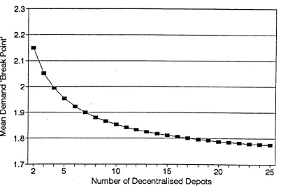
Identification of a limiting 'break-point'

126

6.4.6

A new conjecture

127

6.4.7

Evaluation of the 'general condition'

inequality to test the new conjecture

128

6.5

Extension of the general approach to service-based models

with more than one in stock at each decentralised depot

129

6.5.1

Extension of the general condition for

service disbenefits

129

6.5.2

Application of the 'extended general

condition'

131

6.5.3

Identification of a limiting 'break-point'

6.5.4

A generalisation of the new conjecture

132

6.5.5

Evaluation of the 'extended general condition'

inequality

133

7.

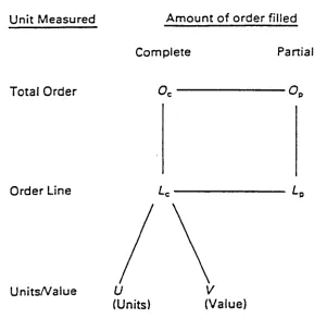
Relationships between Service Level Measures 137

7.1 Introduction 137

7.2 Definition of measures 138

7.3 Previous research on service level measures 140

7.3.1 Unit fill-rate over lead-time 140

7.3.2 The use of a range of measures 140

7.4 Relationships between measures 142

7.4.1 Relationships between measures based on

'complete fill' 142

7.4.2 Relationships between measures based on

'partial fill' 144

7.4.3 Relationships between 'partial fill' and

'complete fill' measures 146

7.4.4 A network of relationships 147

7.5 Implementation issues 148

7.6 illustrative examples 149

7.7 Conclusions ₁₅₂

In

DEMAND DISTRmUTION

FAMILIES

Summary of Part ill ₁₅₄

8.

Demand Distribution Models ₁₅₆

8.1 Introduction ₁₅₆

8.2 The log-zero-Poisson distribution 158

8.2.1 Definition of the log-zero-Poisson

distribution 158

8.2.2 The flexibility of the log-zero-Poisson

distribution 158

8.2.3 Empirical evidence to support the

log-zero-Poisson distribution 159

8.2.4 A biometric analogy 160

8.2.5 The log-zero-Poisson as a 'compound

8.3 Negative binomial distribution 164

8.3.1 Representation of demand by the negative

binomial distribution 164

8.3.2 A

priori

justification of the NBD demand

model 165

8.4 The gamma distribution 167

8.4.1 Representation of demand by a gamma

distribution 167

8.4.2

A priori

justification of the gamma demand

model 168

8.5 The compound Poisson distribution for stationary demand 169

8.5.1

A priori

justification of the compound

Poisson demand model 169

8.5.2 Representation of demand by the compound

Poisson distribution 171

8.6 The compound Poisson distribution for non-stationary

demand 172

8.7 Conclusions 174

9.

Inter-Purchase Time Distribution Models 176

9.1 Introduction 176

9.2 Criticisms of the assumption of 'random' demand from

individual consumers 176

9.2.1 Purchase habit effect 176

9.2.2 Consumption effect 177

9.2.3 Variability in shape of inter-demand

distributions 177

9.3 The geometric inter-purchase distribution 178

9.3.1 A

priori

case for the geometric distribution 178 9.3.2 Empirical evidence on the geometric

distribution 179

9.4.3

Empirical evidence based on inter-demand

times on a stockist

184

9.4.4

Condensed-Poisson demand incidence

distribution

184

9.4.5

Condensed negative binomial demand

distribution

186

9.5

The inverse Gaussian inter-purchase distribution

187

9.5.1

A

priori

case for the inverse Gaussian

distribution

187

9.5.2

Empirical evidence of household purchases

188

9.6

Conclusions

195

9.6.1

Negative exponential inter-purchase

distribution

195

9.6.2

Geometric inter-purchase distribution

195

9.6.3

Erlang inter-purchase distribution

196

9.6.4

Inverse Gaussian inter-purchase

distribution

196

10.

Efficiency and Bias of Estimation Methods

198

10.1

Introduction

198

10.2

Inter-purchase time and demand incidence distributions

200

10.2.1

Inter-purchase time distributions

200

10.2.2

Poisson and binomial demand incidence

distributions

200

10.2.3

Condensed Poisson demand incidence

distribution

200

10.3

Gamma demand distribution

202

10.3.1

Method of moments

202

10.3.2

Maximum likelihood estimation

203

10.4

Negative binomial demand distribution

206

10.4.1

Estimation methods for the NBD

206

10.4.2

Efficiency of the 'means and zeros' method

207

10.4.3

Efficiency of the method of moments

208

10.4.4

Maximum likelihood estimation

211

10.4.5

Bias of method of moments, 'means and

10.5 Condensed negative binomial distribution 213

10.5.1 Method of moments 213

10.5.2 Means and zeros 215

10.6 Log-zero-Poisson distribution 216

10.6.1 Efficiency of the method of factorial

moments 216

10.6.2 Maximum likelihood estimation 217

10.7 Conclusions 218

11.

Empirical Analysis of Demand Distributions 220

11.1 Introduction 220

11.2 Stock management at Pillar Engineering Supplies Ltd 221

11.2.1 Policy objectives 221

11.2.2 SKU categories at Pillar Engineering Supplies 221

11.2.3 Ordering policies

222

11.3 Data for analysis 223

11.3.1 Sample of SKUs 223

11.3.2 Length of data history 224

11.3.3 Data fields extracted 226

11.3.4 Calculation of inter-purchase times, weekly

demand and weekly demand incidence 227

11.3.5 Seasonality of demand 227

11.4 Estimation methods and goodness-of-fit tests 227

11.4.1 Estimation methods 227

11.4.2 Goodness-of-fit tests 228

11.5 Goodness-of-fit of demand incidence and inter-purchase

time distributions 230

11.5.1 11.5.2

11.5.3

Presentation of results

Poisson demand incidence and exponential inter-purchase times

Binomial demand incidence and geometric inter-purchase times

Condensed-Poisson demand incidence and

230

230

11.5.5

Comparison of demand incidence

distributions

234

1l.6

Goodness-of-fit of demand distributions

235

11.6.1

11.6.2

11.6.3

11.6.4

11.6.5

11.7

Conclusions

Negative binomial distribution

Gamma distribution

Condensed negative binomial distribution

Log-zero-Poisson distribution

Comparison of demand distributions

235

236

237

238

240

243

IV

DEMAND VARIANCE LAWS

Summary of Part IV

246

12.

Variance Laws for Inventory Management

248

12.1

Introduction

248

12.2

Variance laws

250

12.2.1

Definition of a variance law

250

12.2.2

Stevens' joint demand model

251

12.2.3

A re-formulation of the joint demand model

253

12.3

Quadratic variance law for compound Poisson demand

255

12.3.1

The stationary mean model: a generalisation

of the re-formulated model

255

12.3.2

12.3.3

Variance law and the effect of dependence of

mean order-size on mean demand incidence

256

Analogous results from insurance mathematics 258

12.4

Condensed-Poisson demand incidence

260

12.4.1

12.4.2

12.4.3

General relationship between variance and

mean of demand

260

Variance law

if

mean order-size independent

of mean demand incidence

261

Comparison with Chatfield and Goodhardt's

12.5 General variance laws 263

12.5.1 Order-size assumptions 263

12.5.2 Relationship between mean order-size and

mean demand 264

12.5.3 Relationship between variance and mean of

order-size 264

12.5.4 General variance law based on 'stationary

mean'model 266

12.5.5

Comparison of the general variance law

with Sherbrooke's law 267

12.5.6 Relaxation of stationary mean assumption

-the steady state model 268

12.5.7

Variance law based on the 'steady state'

model 268

12.6 Conclusions 270

13.

Empirical Analysis of Variance Laws 272

13.1 Introduction 272

13.2 Mean and variance estimation methods 274

13.2.1 Estimation of mean demand incidence 274 13.2.2 Estimation of the standard deviation of

demand incidence

275

13.2.3 Estimation of mean order-size 275 13.2.4 Estimation of the standard deviation of

order-size 276

13.2.5

Estimation of mean demand 276

13.2.6 Estimation of standard deviation of demand 276

13.3 Identification of the most accurate estimation methods 277

13.3.1 Indication of underlying model 277 13.3.2 Testing of one-step ahead forecast accuracy 277 13.3.3 Identification of estimation methods 279

13.4 Heteroscedasticity in variance law estimation 280

13.5

Estimation of the relationship between variance and mean

order-incidence 283

13.5.1

Ordinary least squares estimation 283

13.6

Testing the assumption of independent mean order-size and

mean order-incidence

288

13.7

Estimation of the relationship between variance and

mean order-size

290

13.7.1

Ordinary

least squares estimation

290

13.7.2

Weighted least squares estimation

293

13.8

Estimation of the relationship between mean order-size

and mean demand

298

13.8.1

Ordinary

least squares estimation

298

13.8.2

Weighted least squares estimation

301

13.9

Estimation of the relationship between the mean and

variance of demand

304

13.9.1

Ordinary

least squares estimation

304

13.9.2

Weighted least squares estimation

306

13.10 Conclusions

309

13.10.1

Variance of demand incidence

309

13.10.2

Independence of mean order-size and mean

demand

309

13.10.3

Variance of order-sizes

309

13.10.4

Mean order-sizes

310

13.10.5

Variance of demand

310

14.

Application of Variance Laws in Centralisation Modelling

312

14.1 Introduction

312

14.2 The stationary mean model for centralised demand

313

14.3 Variance of demand incidence

315

14.3.1

Non-correlated demand between depots

315

14.3.2

Correlated demand between depots

315

14.4 Mean order-size

319

14.4.1

14.4.2

14.4.3

Customers' ordering patterns

319

Inappropriateness of EOQ based relationships 320

14.5 Variance of order-sizes 322

14.5.1 Non-identical distributions of order-sizes 322 14.5.2 Identical distributions of order-sizes 323

14.6 Variance of demand 324

14.6.1 General variance law for centralised demand 324 14.6.2 Centralised quadratic variance law as a

special case 324

14.6.3 Testing the centralised variance expression 325

14.7 Conclusions 326

V CONCLUSIONS

15.

Conclusions, Limitations and Further Research 328

15.1 Introduction 328

15.2 Conclusions from part I : inventory amalgamation models 330

15.2.1 Classification of inventory amalgamation

models 330

15.2.2 Safety stock centralisation models 331 15.2.3 Safety stock consolidation models 332 15.2.4 Cycle stock centralisation models 333

15.2.5 Robustness to Economic Order Quantity

assumptions 334

15.3 Conclusions from part Il : inventory service models 335

15.3.1 Benefits and disbenefits of inventory

centralisation 335

15.3.2 Relationships between service-level measures 337

15.4 Conclusions from part ill : demand distribution families 338

15.4.1 Demand distribution models 338

15.4.2 Inter-purchase time distribution models 340 15.4.3 Efficiency and bias of estimation methods 341

15.4.4 Empirical analysis of demand distributions 342

15.5.3

Application of variance laws in centralisation

modelling

344

15.6 Trade-offs between inventory and transport costs

344

15.7 Limitations and further research

347

15.7.1

15.7.2

Theoretical work

Empirical work

347

348

BmLIOGRAPHY

APPENDICES

1.1

Chikan's Secondary Codes

3.1

Mathematical Proofs of Results in Chapter 3

5.1

Mathematical Proofs of Results in Chapter 5

6.1

General Conditions for Service Benefits

I

Disbenefits

6.2

Limiting Conditions for Service Benefits

I

Disbenefits

6.3

Identification of a Limiting 'Break-Point'

7.1

Mathematical Proofs of Results in Chapter 7

LIST OF TABLES

Chapter 3:

Salety Stock Consolidation Models

3.1

Mahmoud's PE Matrix (1992)

(from an example by

Zinn,

Levy and Bowersox (1989»

Chapter 4:

Cycle Stock Centralisation Models

4.1

Proportion of maximum cycle stock savings

if

the two decentralised

mean demands are not identical

4.2

Size ratios above which predicted savings are not attained

4.3

Proportion of maximum cycle stock savings attainable if mean demands

are not identical (multi-depot case)

4.4

Size ratios above which given percentages of savings predicted by the

cycle stock square root law are not attained

Chapter 6:

Benefits and Disbenefits or Inventory Centralisation

6.1

Mean demand break-points for service benefits

6.2

Mean demand break-points for service benefits from centralisation

6.3

Probability of stock-out break-points for service benefits from

centralisation

Chapter 7:

Relationships between Service Level Measures

7.1

Six service level measures

7.2

Key ratio (u

d

J./lu

uJ for each client group and movement class

7.3

Sensitivity to movement category for each client group

7.4

Sensitivity to client group for each movement category

Chapter 8:

Demand Distributions for Inventory Modelling

8.1

First analogy between the hatching of larvae and the ordering of items

8.2

Second analogy between the hatching of larvae and the ordering of

Chapter 9: Inter-purchase Time Distributions

9.1 Chi-square 'goodness of fit' statistics for toothpaste purchase data

9.2 Acceptance or rejection of models for toothpaste purchase data

Chapter

10:

Efficiency of Estimation Methods for Parameters of Demand Distributions

10.1 Sample sizes required for ML bias of less than 10% for Gamma shape parameter

10.2 Parameter values of NBD in Banerjee & Bhattacharyya's study 10.3 Efficiency of moment estimator in Kwan's study

lOA Schmittlein and Morrison's comparison of CNBD exponent estimators

10.5 Schmittlein and Morrison's comparison of CNBD scale parameter estimators

Chapter 11: Empirical Analysis of Demand Distributions

11.1 Proportion of SKUs sampled

11.2 Estimation methods

11.3 Categorisation of SKUs by speed of movement

11.4 Percentage of SKUs with demand incidence fitted by the Poisson distribution

11.5 Percentage of SKUs with demand incidence fitted by the binomial distribution

11.6 Percentage of SKUs with demand incidence fitted by the condensed-Poisson distribution

1l.7 Percentage of SKUs with demand fitted by the negative binomial distribution

11.8 Percentage of SKUs with demand fitted by the gamma distribution

1l.9 Percentage of SKUs with demand fitted by the condensed negative binomial distribution

11.11 Example of poor performance of 'means and zeros' in NBD estimation for fast moving SKU s

11.12

Example of good performance of 'means and zeros' in NBD estimation for slower moving SKU s

11.13 Example of good performance of maximum likelihood in Ganuna estimation for fast moving SKUs

11.14 Example of poor performance of 'means and zeros' in CNBD estimation for faster moving SKU s

Chapter 12: Variance Laws for Inventory Management

12.1

Analogy between insurance claims and demand for inventory

Chapter 13: Empirical Analysis of Variance Laws

13.1

Total squared errors (EWMA comparison)

13.2

Total squared errors (MA comparison)

13.3

Recommended estimation methods

13.4

Order-incidence incidence variance -mean R2 measure 13.5 Order-incidence variance - mean parameter estimates

13.6

Independence of mean order size and mean order-incidence

13.7

Order-size variance - mean R2 measure

13.8

Order-size variance - mean parameter estimates 13.9 Order-size variance-mean parameter estimates

(weighted least squares)

13.10

Mean order-size - mean demand R2 measure

13.11

Mean order-size - mean demand parameter estimates

13.12

Mean order-size - mean demand parameter estimates (constant term constrained to unity)

13.14

Demand variance - mean R2 measure

LIST OF FIGURES

0.1

Logical interdependence

of the five parts of the thesis

1.1

Naddor's classification system

1.2

Aggarwal's classification system

3.1

Optimal consolidation of four depots

4.1

Proportion of maximum cycle stock savings attainable

6.1

Benefits/disbenefits

for the two-depot case with one item in stock

6.2

Mean demand break-points for service benefits

7.1

Network of relationships between service-level measures

10.1

Efficiencies of moments estimators for the gamma distribution

10.2

Large sample efficiencies for 'means and zeros'

10.3

Large sample efficiencies for the method of moments

10.4

Large sample efficiencies for moments and 'means and zeros'

13.1

Kurtosis

(BJ -

skewness

(B1)

diagram

13.2

Mean and variance of order-incidence for PES data

13.3

Residuals from order-incidence variance - mean relationship (OLS)

13.4

Order-incidence variance - mean relationship (WLS)

13.5

Mean order-size and mean order-incidence for PES data

13.6

Mean and variance of order-size for PES data

13.7

Mean and variance of order-size for PES data

(two outlying observations removed)

13.12

Mean order-size and mean demand for PES data

13.13

Residuals from mean order-size - mean demand relationship (OLS)

13.14

Mean order-size - mean demand relationships

GLOSSARY

Amalgamation

An

umbrella term for ' centralisation' and 'consolidation'

(defined

below).

Centralisation Amalgamation of inventories from more than one depots to one depot.

Complete Line

Fill

Proportion of total lines which are filled completely (notation -

Le>

Complete Order

Fill

Proportion of total orders which

are

filled completely (notation - Oc)

Consolidation Amalgamation of inventories from more than one depot to fewer depots but not to one depot.

Cycle stock Those stocks held to achieve economies of scale in ordering and production (notation - CS).

Demand Demand occurs when a customer orders a product, regardless of whether the demand is completely or partially satisfied or not satisfied at all. The total number of units ordered is defmed

as

'demand'.

Demand Incidence The total number of order occasions is defined

as

'demand incidence'.

Economic Order Quantity (EOQ)

Amount ordered to satisfy a cost minimisation

function which takes into account ordering and holding costs.

Inter-correlations Correlations between demands on depots from different sub-consolidations.

Intra-correlations Correlations between demands on depots from the same sub-consolidation.

Joint demand model A model of demand which reflects variations in demand for an SKU attributable to both individual SKU effects and joint effects (such

as

market fluctuations) which affect many SKUs.

Operationalisation Translation of abstract concepts into measures enabling observations to be made.

Partial Line Fill

Partial Order Fill

PES Portfolio Effect Portfolio Cost Effect Portfolio Quantity Effect Return on investment (ROn ROQ Safety stock Service level SKU

Square root law

Proportion of total lines which are filled (at least) partially (notation -

r,,).

Proportion of total orders which are filled (at least) partially (notation

-o,»

Pillar Engineering Supplies Ltd.

Denotes the percentage saving in safety stock arising from centralisation or consolidation.

Reduction in cost (including holding cost, transportation cost, investment cost and procurement cost) arising from inventory amalgamation.

Reduction in stock quantity arising from depot amalgamation.

Ratio of profit before tax to total equity, including inventory.

Order quantity which maximises Ra!.

Those stocks held as a buffer against unforeseen fluctuations of demand (notation - SS).

A measure of the availability of stock to customers.

Stock keeping unit

The total stock in a system is proportional to the square root of the number of locations at which a product is stocked.

Super consolidation An alternative name for 'centralisation'. Sub consolidation

Total stock

Unified Order Quantity

Unit fill rate

Value fill rate

Variance law

An alternative name for 'consolidation'.

The total of cycle stock and safety stock (notation - TS).

An order quantity which optimises the total costs across the whole of the distribution chain.

Proportion of units ordered filled from stock (notation - U).

Proportion of value of units ordered filled from stock (notation - V).

ACKNOWLEDGEMENTS

There are many people who have helped and supported me throughout the period of

my part-time PhD study but without the following the road would have been much

harder.

I would especially like to thank Roy Johnston, my supervisor, for our meetings which

I found

to

be unfailingly challenging, stimulating and encouraging. His advice has

been much valued.

I am indebted to Alan Thompson and Stuart Coggins, of Pillar Engineering Supplies,

for helping me to obtain

data

on demand histories of a large sample of stock keeping

units. I am also grateful

to

my employers at Buckinghamshire College for financial

support and reduction in teaching load. particularly during the sabbatical semester,

which has been invaluable in allowing me to complete the thesis.

DECLARATION

Thirteen of the fifteen chapters

in

this thesis have not been published before. Two

chapters,

in

slightly different form, have been published as journal articles.

The

details are given below.

*

Chapter 7 is based on :

BOYLAN, IE and JOHNSTON, FR (1994) Relationships between service

level measures for inventory systems.

J

Opl Res Soc,

45, 838-844.

*

Chapter 12 is based on :

BOYLAN, IE and JOHNSTON, FR (1996)

Variance laws for inventory

management

Int

J

Production Economics,

45, 343-352.

Both articles are the product of original research by the first-named author.

The

second-named author was included in recognition of his constructive comments and

criticism, acting

in

his capacity as PhD supervisor.

SUMMARY

The motivation for this research arose from two projects in which the author advised

on inventory centralisation. Since it was found that the literature was of limited value,

inventory centralisation was identified as a suitable topic for research.

Operationalisation is not adequately addressed in the literature on centralisation

models. 'Operationalisation' denotes the translation of abstract concepts such as

'inventory service' into measures enabling observations

to

be recorded.

In

the

literature, 'inventory service' is often equated to 'probability of stock-out' but many

other measures are used in practice. This thesis presents a network of relationships

between six commonly used measures. This is useful when decentralised depots do

not share a common measure, or when the measure changes after centralisation.

This thesis argues that, under all circumstances which arise in practice, it will be

possible to achieve inventory availability benefits from centralisation with no added

investment in stocks.

A

counter-example to the universal application of this rule have

been presented in the literature but it is shown that such counter-examples are

artificial.

Since savings from centralisation may be offset by increases in transport costs, the

reduction in stock-holdings needs to be estimated.

The models presented in the

literature assume that the estimation of demand variance and the correlation of demand

between depots is not problematic.

In

practice, reliable estimates may be difficult to

obtain, particularly for slow-moving items. Consequently, it is difficult to decide

which items should be centralised and which, if any, should not This thesis proposes

a 'quadratic variance law' approach', linking the variance of demand to its mean.

This approach is underpinned by a model which allows correlation effects to be taken

into account

The 'variance law'

approach is a contribution towards the

operationalisation of centralisation models, since reliable estimates of mean demand

are easier to obtain than estimates of variance and correlation.

The 'quadratic variance law' is examined empirically using a sample of 230

stock-keeping units from an engineering supplies company. The approach is shown to be

well-supported by the data. All the model assumptions are supported except one. The

postulated independence between mean order-size and mean demand is rejected since

a weak correlation was found. However, the simpler quadratic law is found

to be

INTRODUCTION

In

this introductory section of the thesis. four issues will be addressed :

1.

The importance of inventory centralisation to organisations.

2.

The principal shortcomings of published models and criteria for •good'

centralisation models.

3.

The structure of the thesis.

4.

The methods used in the research undertaken.

This material will provide a background to the research and the main arguments to

be

developed. A summary of the research findings is given in chapter 15.

0.1 Business context

Logistics is a matter of strategic importance for organisations since it can contribute

to competitive advantage by cost reduction and service improvement.

In

this section.

the role of inventory centralisation in achieving competitive advantage is discussed.

0.1.1 Benefits of inventory centralisation

stock-holdings to one location in southern Sweden (later relocated to Belgium). The

centralisation reduced the value of inventory holding from 29% to 20% of sales.

Substantial reductions in warehousing costs were also achieved. Abrahamsson claims

that, despite the introduction of some air freight, transportation costs remained constant.

Although the above discussion is limited to one company, Evans (1993) found that

25% of respondents to a KPMG survey cited 'centralisation of distribution' as a

'response to market pressures'. The sample for the

KPMG

survey consisted of 153 directors of leading European companies.

The second reason why inventory centralisation is important is that a more consistent

level of inventory service may be provided to all customers. If stocks are de-centralised, then different availability levels may be observed at the depots. It is even

possible that the same availability may be achieved according to a formal measure and

yet a worse service may be offered to some customers. For example, in a study of

European distribution of Austin Rover parts, Eastburn and Nockold (1986) found that,

"the P&A stock control system ... is wilfully (and cleverly) abused in Bologna where

they stock-pile the very cheap pans in preference to the very expensive pans in order

to achieve the target

92%

availability with as little investment as possible. Hence,

they would be able to supply the nuts and bolts to attach a new alternator, but could

be out of stock of the alternator itself."

If,

on the other hand, stocks are centralised,

then the company service policy can be implemented more straightforwardly and all

0.1.2 Implementation of centralisation

The first step in examining centralisation options is to identify customer lead-time

requirements.

If

customers require delivery within 48 hours of order submission, then

a detailed analysis of lead-times will enable the minimum number of stock-holding

points to be identified.

Lead-times may be split into two components : physical lead-time and administrative

lead-time. Within the EU, the relaxation of border controls and the opening of the

channel tunnel have contributed towards shorter physical lead-times. More

significantly, advances in information systems have enabled substantial reductions in

administrative lead-times to be achieved. For example, Taylor (1991) describes how

Unipart Group Ltd achieved significant improvements in its delivery service to parts

wholesalers. The new service was based on daily receipt of stock-orders and provided

a reduction in turn-round time from receipt of order to delivery from five working

days to just one working day. Implementation of software allowing wholesalers to

interface directly with the Unipart mainframe computer enabled direct transmission of

orders. The new system reduced preparation time by wholesalers and eliminated the

need to input orders from hard copy at Unipart, thereby cutting the order cycle time.

Reductions in order-cycle times such as these have given many companies greater

scope for centralisation.

In

conclusion, centralisation of inventories has been achieved by many organisations,

is a feasible approach for many others, and may yield significant cost reductions and

0.2 Modelling of inventory centralisation

0.2.1 The need for inventory centralisation models

An inventory centralisation model enables a manager to obtain estimates of the

reduction in stock-holding which would result from centralisation. This

is

useful since it provides a forecast of the capital which will be freed for other activities. In the Atlas Copeo case, for example, it was intended to use the money saved by inventory

reductions to boost the marketing operations of the national sales companies.

Inventory centralisation models may also be used to compare different options for

inventory amalgamation. Abrahamsson (1993) argues that such models

are

un-necessary and a 'time based distribution' approach should be used: "...

the lead-time

is the only variable to consider to calculate the number of warehouses."

This

assumes that the total cost curve always rises as the number of warehouses increases.

This assumption is valid if transport costs do not rise as a result of centralisation, as

in the case of Atlas Copco.

At Atlas Copco, centralisation resulted in a large number of small deliveries to a large

number of customers. In these circumstances, centralised transport costs should be

greater than in the decentralised scenario. One possible explanation for the constancy

of transport costs is that, since inventory availability was very poor at the

decentralised depots (only 70%), significant costs of expediting were saved by

centralisation, offsetting the increases in delivery costs. Ifhigher availabilities were attained at the decentralised depots, then transport costs may have been considerably

This discussion highlights the problems in generalising the findings from a case-study.

Since a number of variables change after centralisation, it is not possible to claim that

total logistics costs always reduce as a result of inventory centralisation. A deeper

understanding is afforded by modelling the effect of centralisation on inventory,

warehousing and transport costs in each individual case.

Then, together with an

assessment of the impact on inventory availability, a more informed decision may be

made.

0.2.2 Weaknesses of published centralisation models

A detailed review and critique of published models is given in part I of the thesis.

Three issues, in particular, have been under-researched in the literature :

1.

The measurement of service levels.

It is generally assumed in the inventory centralisation literature that

'probability of stock-out during lead-time' is the measure used.

However,

many organisations use other measures such as line-fill or order-fill.

For

centralisation models to be useful in these circumstances, or in situations where

different measures are employed at different decentralised depots, a set of

relationships between service levels is required.

2.

The estimation of demand variance.

should be considered for this category of inventory. More accurate estimation

of demand variance would allow a better assessment to be made of which

SKUs should be centralised and which should not

3. The

estimation of demand covariance.

Again, few published models discuss the estimation of demand covariance

between depots. The same estimation difficulties occur in the circumstances

highlighted for demand variance. ITthe effect of demand covariance could be

estimated more accurately, this would enable the assessment of stock

centralisation to be improved when there are some correlations between

demands at decentralised depots.

0.2.3 Criteria for 'good' centralisation models

A 'good' inventory centralisation model satisfies a number of criteria. Firstly, the

model assumptions should not be too restrictive. Early publications assumed equal

mean demands at all decentralised depots and no correlation between demands. Both

of these assumptions are unlikely to hold in practice.

The second criterion is that the model assumptions should be clearly stated. For

example. some users of the 'square root law', to be discussed in chapter 2, may be

unaware of the assumptions behind the 'law'. Not all publications on this 'law' give

a comprehensive list of model assumptions.

order to assess the effect of inventory centralisation on demand variability. Without

such a structure, 'what

if'

analyses cannot be performed.

The

final

criterion is that the method of estimation or measurement of all variables included in the model formulation is specified. Without such a specification, a model

0.3 Thesis structure

0.3.1 Overall structure

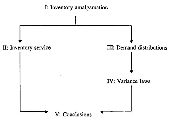
The thesis is divided into five parts, namely:

Part I

Inventory amalgamation models

Part II

Inventory service models

Partffi

Demand distribution families

PartN

Demand variance laws

Part V

Conclusions

[image:38.521.83.434.437.686.2]

The logical interdependence of the thesis components is summarised in figure 0.1 :

Figure 0.1

Logical interdependence of the five pans of the thesis

I: Inventory amalgamation

1

1

ID: Demand distributions

1

II: Inventory service

IV: Variance laws

0.3.2 Inventory amalgamation models

This part of the thesis contains a detailed literature review and critique of previously

published models. The models are assessed with particular reference to the clarity of

their stated assumptions. Where necessary, assumptions are corrected or expanded,

with the aid of a classification system for inventory amalgamation models. In some

instances, the models are corrected for mathematical errors.

It is found that, although early models had quite restrictive assumptions. later

generalisations have overcome many of these limitations. However, the three issues

of service measures, variance estimation and covariance estimation, mentioned in

sub-section 0.2.2, are identified as requiring further research.

0.3.3 Inventory service models

Inventory service models are considered from two perspectives in part IT of the thesis.

Firstly, the effect of centralisation on service is examined. The conditions under

which service benefits occur are delineated. It is found that the conditions under

which disbenefits will result are unlikely to occur in practice. These findings are

conjectural since complete mathematical proofs have not yet been obtained.

The second perspective from which service models are viewed is the measurement of

service itself. Many different measures are used in practice and it may happen that

measures vary at decentralised depots or will change after centralisation. To overcome

these difficulties, a 'network of relationships' between six commonly used measures

0.3.4 Demand distribution families

The third part of the thesis, on demand distribution families, is a precursor to the

fourth part of the thesis, on demand variance laws, as shown in figure 0.1.

It is argued that many proposed distributions lack any underpinning theory to justify

their use as demand distributions; the gamma is an example of such a distribution.

Some proposed distributions are examined from a theoretical standpoint and possible

underlying mechanisms are suggested as appropriate. It is shown that the compound

Poisson family of distributions possesses attractive theoretical properties for demand

modelling.

Estimation issues are considered and a number of demand incidence and demand

distributions are tested against empirical demand data on a sample of 230 SKUs from

Pillar Engineering Supplies Ltd. It is found that Poisson demand incidence is well

supported by the data, as is negative binomial demand.

0.3.5 Demand variance laws

The fourth part of the thesis follows on from part Ill, by establishing demand variance

laws based upon compound Poisson demand. The variance of demand is shown to be

a quadratic function of the mean demand under certain assumptions.

mean demand. However, the quadratic variance law is found to

be

more appropriate for the data than a more complex expression which includes an allowance for the

correlation between mean order-size and mean demand.

0.3.6 Conclusions

In the final part of the thesis, the conclusions are summarised, limitations of the research are identified and avenues for further research are outlined.

One of the main conclusions of the research is that a quadratic variance law may be

used to estimate demand variance. The variance law allows the effect of demand

covariance to be taken into account automatically.

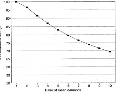
The variance law predicts that as the mean demand rises, the proportional

stock-savings from centralisation decrease. The predictions allow a comparison with

marginal increases

in

transport costs to be made, thus identifying those SKU s which

0.4 Methodology

0.4.1 A deductivist approach

The thesis is characterised by a deductivist approach.

Theories of inventory

amalgamation, inventory service, demand distributions and demand variance 'laws'

have been deduced from various assumptions. The assumptions have been examined

in two different ways. Firstly, they have been checked for their general plausibility:

do they make sense in an inventory context?

Secondly, they have been tested

empirically: are they supported by data from a real organisation ?

An alternative approach is to analyse inventory data before and after centralisation and

to infer some general principles from the observations. Abrahamsson's (1993) 'time

based distribution' principle, discussed in sub-section 0.2.1, is a good example of the

dangers of the inductive approach. After depot centralisation, a number of variables

may change in addition to the number of inventory locations. In Abrahamsson's case,

the level of inventory availability increased markedly. This may have affected the

transport costs and casts doubt on the general proposition that total logistics costs

always decrease as the number of inventory locations decrease.

on inventory amalgamation has not progressed beyond the first stage of Popper's

method. The purpose of this thesis is to 'operationalise' centralisation models and to

test the underpinning theory.

0.4.2 Service level measures

A set of relationships between inventory service measures is presented in chapter 7.

Since the relationships are algebraic links of

definitions,

they are tautological.

However. they have been formulated in such a way that only those variables most

likely to

be

available in practice have been included. Thus, the relationships were

operationalised.

Empirical testing is not relevant in this case since the algebraic

formulae are tautological.

0.4.3 Demand variance laws and demand distributions

0.4.4 Amalgamation models

The amalgamation models presented

in

chapter 14 are based on the theories of

compound Poisson demand and a quadratic variance - mean demand relationship. The

quadratic variance law provides an operationalisation of the amalgamation models.

Although both the compound Poisson distribution and the quadratic variance law have

been tested empirically. the amalgamation models have not been subject to empirical

PART!

INVENTORY

Summary of Part I

In this part of the thesis, a literature review and critique of previous work on inventory

amalgamation is provided. The term 'amalgamation' covers both 'centralisation' to

one depot and 'consolidation' to more than one depot

In the first chapter, a classification system for inventory amalgamation models is

developed. The system is used as a framework throughout the literature review. The

classification provides a structured approach to the identification of the main model

assumptions. This is an important issue in amalgamation modelling since such clarity

has not always been achieved in this field of research.

Chapters 2 and 3 contain a detailed literature review and critique of safety stock

amalgamation models. Work by Zinn, Levy and Bowersox (1989) on this problem

is reviewed and, using the classification system, shown to be mis-categorised as a

cost-driven model when

it

is actually a service-driven model. Some corrections to

previously published papers are given, notably the preference rule between different

types of consolidation (Mahmoud (1992» and the centralisation model for variable

lead-times (Tallon (1993».

Estimation of demand variance and covariance are highlighted as requiring further

work. The models reviewed assume that these estimates will

be

readily available but

there are many situations in which estimation may

be

difficult This issue is examined

theoretically and empirically in part IV of the thesis.

In

chapters 4 and 5, cycle stock centralisation models are examined. Estimation issues are not discussed since estimation of mean demand is less problematic than estimation

of demand variance and covariance. The robustness of the cycle stock square root law

to unequal mean demands is examined. Also, in chapter 5, the robustness of the

Economic Order Quantity (EOQ) approach is discussed, with reference to its

application in centralisation modelling. It is shown that some of the limitations of the

EOQ model at fixed locations do not apply to centralisation models, assuming

parameters are unchanged by centralisation. However, the use of the alternative

criterion of return on investment produces quite different results. Lower and upper

CHAPTER 1

Classification of Inventory Models

1.1 Introduction

1.1.1 Summary

In this chapter, classifications of inventory models will be reviewed. Classification

systems have been designed for models of inventories at fixed locations but it will be

argued that inventory amalgamation models require their own classification. The lack

of such a classification is remedied by a new system, based on previous work on fixed

location inventories but specifically adapted for amalgamation models. In the

following three chapters, the new classification system will be applied to two types

of inventory amalgamation: 'centralisation', where the inventories are amalgamated

in one location, and 'consolidation', where the inventories are amalgamated in more

than one location.

1.1.2 Reasons for classification

Before proceeding to the detailed review and proposal, it is worth reflecting on why

a classification system is needed for inventory amalgamation models. There are two

main reasons. First, such a system would help the modeller appreciate the place of

each model within the overall body of research. The case for such a classification

system for fixed-location inventory models is overwhelming, since many hundreds of

as there are fewer published models. However, it

will

be shown that some researchers

have incorrectly placed their own work within the discipline and it will be argued that

greater clarity of assumptions is needed. One way of achieving this is by adopting a

formal classification system which encapsulates essential model assumptions.

1.2 Review and critique of classification systems

Clearly, there is no definitive way in which inventory models should be classified and

a number of authors have produced systematic classification systems of varying

degrees of complexity. Three publications

in

this area are reviewed in this section:

Naddor (1966), Aggarwal (1974) and Chikan (1990).

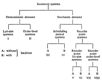
1.2.1 Naddor's classification

[image:50.521.77.433.323.607.2]

Naddor's (1966) classification of inventory models is shown in Figure 1.1 :

Figure 1.1

Naddor's classification system

Inventory systems

I

I

Stochastic demand 1 Deterministic demand Lot-size systems J Order-level systems IJ Scheduling Reorder period point systems systems 1 1

A B Reorder Reorder

III IV point point

lot-size order-level systems systems

1 1

-II

A B A B

V VI VII VIII A: Without}

leadtime

B: with

Naddor's classification system is quite rudimentary. It ignores three issues which are

important in fixed-location and amalgamation models alike, namely : the system

stochastic) and the multi-depot situation.

1.2.2 Aggarwal's classification

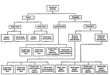
[image:51.521.67.445.250.507.2]

Aggarwal (1974) produced an alternative classification system, shown

in

Figure 1.2

below, based on similar principles to the work of Naddor :

Figure 1.2

Aggarwal's classification system

Inventn".

sys.ems

SIl.ic

I

Deterministic

I

SinJle item multi-echelon muhi-loca.ion Mu1Ii-ilem 1 multi-location mul.i-«helon

Known _Unknown

I

dnnand demand

di~tribution distribu.ion

I I

:1

multi-IocationlMuhi·i.em

'I

Ion multi-echelon

I I I

Single-item Muhi·i.em _{mul1i-echel(ln}Sinlde-item Multi-item murti-single. lingle.

mullt- loca.ion loca.ion location _{location mul ti-echelon}

1 Muhi·i.em singl ..

loea-tit'n '---'

Sin"le-item

!rinJIe.loca-lion

1.2.3 Chikan's classification

A more comprehensive classification of fixed-location inventory models was given by

Chikan (1990). Chikan

uses ten 'main codes'

(Mel

to

MelO)

to categorise inventory models:

MCl

Number of items stored in the system

Code

1

Code

8

one item stored

several items (ie more than one) stored

MC2

Number of stores in the system

Code 1 Code 8

one store in the system several stores in the system

MC3

Character of the inflow (input) process

Code 0

Code 1

input is deterministic input is stochastic

Input is said to be deterministic ifall elements of the input process are known with certainty. According to Chikan's definition, ifany uncertainty exists, then the inflow is considered to be stochastic.

MC4

Character of the outflow (output) process

Code 0

Code

1

output is deterministic output is stochastic

The same considerations apply as to inputs. The deterministic or stochastic character of demand determines the character of the outflow.

MC5

Way of treating time in the system ('dynamics' of the system)

Code 0

Code

1

the model is static the model is dynamic

of the same objective function taken at some other time. Otherwise, the model is said to be ' static' .

MC6

The objective of the system

Code 0 Code

1

Code

2

optimisation model reliability model descriptive model

The optimisation model category covers such criteria

as

cost minimisation, discounted cost minimisation and income maximisation. 'Reliability models' are driven by demand satisfaction objectives. Finally, 'descriptive' models describe the reaction of an inventory system to impulses from the 'external world'.

MC7

Operation mechanism of the system (ordering rule)

Code

0

Code 1 Code 2 Code 3 Code

4

Code 5 Code 6 Code 8 (t, S) (~, S)

(s,q) or (s,q,,)

(sp' q)

(t,q), (~, q) or (t, q,,) (s, S) or (s, Sp)

(sp, S) (t, Sp) where t

s

q S fixed order-interval re-order point fixed order quantity order-up-to point

p fixed parameter

A 'fixed parameter' is not reviewed at the same time that the stock-ordering decision is reviewed.

MC8

Mode of review

Code 0 Code 1 Code 2

no inventory reviewing periodic review

MC9

Treatment

of

shortage

Code 0 Code 1 Code 2

shortage not allowed

shortage allowed, demand back-ordered shortage allowed, lost sales

Models with 'shortage not allowed' are relevant to situations with deterministic demand or stochastic demand constrained to a maximum value.

MC1D Lead-time

Code 0 Code 1 Code 2 Code 3 Code 4

zero lead-time constant lead-time

variable lead-time (but known in advance) stochastic lead-time

fulfilment in more than one lot, or continuously

A distinction is made between two cases where lead-times vary over time. Code 2 is used for situations when the lead-time is known and code 3 for when the lead-time is not known in advance.

In addition to the ten 'main codes' summarised above, Chikan devised a number of

'secondary codes', summarised in Appendix 1.1.

As an illustration of the main code system, suppose that there is a single store, single

item, static optimisation model for a periodic (s,q) system. The model is based on

deterministic inputs, stochastic demand, stochastic lead time and it is assumed that

there will be lost sales if orders are unfilled. This model would be coded :

110

1 002

123

A criticism of this representation is that it is difficult to recognise a model represented

The most significant omission in Chilean's system

is

the classification of multi-echelon models. A secondary factor of 'connection between the stores' is included in the

classification (see Appendix 1.1). Three codes are identified: no connection between

the stores (code 0), linear connection between the stores (code 1) and parallel stores

connected to a central store (code 2). However, this categorisation cannot capture the

richness of multi-echelon inventory systems since the number of levels in the system

is restricted to a maximum of two. Consequently, the arborescent structure of many

multi-echelon systems cannot be represented within the classification.

Another omission in the classification is that no account is taken of the presence, or absence, of correlation between demands at different stores. At item-level, if lateral

supply between depots is permitted, then this issue is relevant. In the context of inventory centralisation, demand correlation assumptions are always relevant.

In this section, the factors used in three classification systems have been examined.

Since Chilean's system is the most comprehensive, it

will

be used as the basis for a

classification of centralisation models. As some factors are omitted by Chikan, these

1.3 Proposed classification of amalgamation models

In

this section, Chikan' s classification system will be used as a basis for developing

a classification of amalgamation models. Factors which require coding for

fixed-location models but not for amalgamation models will be removed. Factors not coded

by

Chikan

but needed for amalgamation models

will

be highlighted and included in the new system. A 'user-friendly' notation for classification will be developed

throughout this section.

1.3.1 Principle of parsimony

In deciding which factors to include in the classification system, a principle of

parsimony is adopted and the number of factors used for the classification is kept to

a minimum. By taking this approach:

*

the essential aspects of a model are covered

*

non-essential aspects may be given secondary codes, as in Chilean's system, without confusing the main classification.

1.3.2 Number of items

Chilean's single-item / multi-item flag requires re-interpretation for amalgamation

models. In such models, the 'multi-item' case may refer to

aggregation

across a

number of items, or to the treatment of aggregate inventory

as a whole,

without

reference to individual SKUs. A number of examples of the former approach are

given in chapters 2 and 4. An example of the latter approach is given by Johnston et

Stock Cover (C)

=

Total average stock

Average monthly demand

A 'response equation' was found (Johnston et al (1988a), (l988b», of the form :

C

=

30

+

a.D

+

~D2

+

a

3

R2

+

a

4

L2

+

a,E2

+

~RL

+

~RD

+

asRE

+

~E

+

a10LD

+

all ED

where

D

=

l/F and F is average monthly demand per item

R is review time

L is lead-time

E

=

exp«S-IOO)/lO) and S is service level, expressed as a percentage.

Such an approach will

be

termed 'GROSS', since the relationships are derived from

inventory as a whole. The alternative approach

to

multi-item modelling, where results

are derived from relationships at item level, will be termed ' AGGREGATE'.

The

distinction between the two categories is intended

to

avoid confusion.

The options are amended accordingly :

SKU

model of stock for an individual SKU

AGGREGATE

model of stock derived for a single SKU and aggregated over

a set of SKUs.

GROSS

model of stock derived from inventory as a whole.

'GROSS' models, which will not be covered further in this thesis, are identified as an

area for further research.

1.3.3 Number of stores : a redundant factor