University of Warwick institutional repository: http://go.warwick.ac.uk/wrap
This paper is made available online in accordance with
publisher policies. Please scroll down to view the document
itself. Please refer to the repository record for this item and our
policy information available from the repository home page for
further information.
To see the final version of this paper please visit the publisher’s website.
Access to the published version may require a subscription.
Author(s): G. ROWLANDS, G. BRODIN and L. STENFLO
Article Title: Exact analytic solutions for nonlinear waves in cold plasmas
Year of publication: 2008
Link to published version:
doi:10.1017/S002237780700699X Printed in the United Kingdom
569
Exact analytic solutions for nonlinear waves in
cold plasmas
G. R O W L A N D S
1, G. B R O D I N
2and L. S T E N F L O
2 1Department of Physics, University of Warwick, Coventry, CV4 7AL, UK2Department of Physics, Ume˚a University, SE-901 87 Ume˚a, Sweden
(Received 9 October 2007 and in revised form 5 November 2007, first published online 10 December 2007)
Abstract. Large amplitude plasma oscillations are studied in a cold electron plasma. Using Lagrangian variables, a new class of exact analytical solutions is found. It turns out that the electric field amplitude is limited either by wave breaking or by the condition that the electron density always has to stay positive. The range of possible amplitudes is determined analytically.
In view of the many technological applications of low-temperature bounded plas-mas, there has recently been an increased interest in this subfield of plasma physics. It is in this connection necessary to study large-amplitude disturbances of the oscillating quantities. The theory of nonlinear plasma waves, which was reviewed by Infeld and Rowlands a few years ago [1], concerns to a large extent studies of wave disturbances by means of expansions in the wave amplitudes. This leads to truncated approximate solutions. However, there are a few cases that can be solved exactly [1, 2]. In the present paper we point out another new interesting exact solution of the electron fluid equations. Such solutions can be used as a means to test numerical codes in regimes where it is usually difficult to determine their accuracy.
The method is described in [1, Sec. 6.4]. The basic equations describing one-dimensional large-amplitude plasma oscillations in a cold electron plasma with immobile ions are
∂n ∂t +
∂(nu)
∂x = 0, (1)
∂u ∂t +u
∂u ∂x =−
e
mE (2)
and
∂E
∂x = 4πe(n0−n), (3)
wherenis the electron density, uthe electron velocity,Ethe electric field,n0 the
ion density,ethe elementary charge andmthe electron mass. The above equations can be combined to give
∂E ∂t +u
∂E
570 G. Rowlands, G. Brodin and L. Stenflo
Next we change the Eulerian variablest, xto the Lagrangian variablesτ, ξwhere t=τ andx=ξ+0τu(ξ, τ)dτ. Then we have
∂ ∂t → ∂ ∂τ − u R ∂ ∂ξ, ∂ ∂x → 1 R ∂ ∂ξ,
whereR= 1 +0τ[∂u(ξ, τ)/∂ξ]dτ. From the above relations we find that without approximation (4) can be rewritten as
∂2E
∂τ2 +ω 2
pE= 0, (5)
where ωp is the unperturbed plasma frequency ωp = (4πn0e2/m)1/2. The most
general solution to (5) isE(ξ, τ) =A(ξ) cos(ωpτ) +B(ξ) sin(ωpτ). If at timet= 0
(τ= 0, ξ=x),E(x, t) =E(ξ,0)andu(x, t) =u(ξ,0), then for allτandξ
E(ξ, τ) =E(ξ,0) cos(ωpτ) +
mωp
e u(ξ,0) sin(ωpτ). (6) Furthermore, we have
x=ξ+u(ξ,0)
ωp
sin(ωpτ)−
eE(ξ,0)
mω2
p
[1−cos(ωpτ)] (7)
and the relation
n(x,0) =n0−
1 4πe
∂E
∂x(x,0) (8)
such that the initial conditions are described by only two arbitrary functionsE(x,0) andu(x,0).
In [1] two distinct solutions were examined in detail withu(x,0) = 0:
1. E(x,0) =asin(kx)whereaandkare constants;
2. n(x,0) = n0[1 +rf(x)] wherer is a dimensionless constant and the function
f(x) is f(x) = 1 for 0 x < π/2k, f(x) = −1 for π/2k x < 3π/2k and f(x) = 1for3π/2kx <2π/k.
In the present paper we consider again the case ofu(x,0) = 0but with
E(x,0) =
aexp(−κ1x) for0< x,
bexp(κ2x) forx <0,
wherea, b, κ1 and κ2 are constants. The major problem is obviously to invert the
(x, ξ)transformation. With the above initial conditions we now have to solve
x=
ξ−aβ(τ) exp(−κ1ξ) forξ >0,
ξ−bβ(τ) exp(κ2ξ) forξ <0,
where β(τ) = [1−cos(ωpτ)]e/mω2p. To solve these equations we introduce the
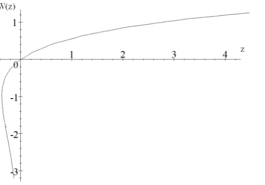
Figure 1.A plot of the real branch of the Lambert function.
We now find that the relation between xandξforξ >0can be written in terms of the Lambert function as
ξ=x+ 1
κ1
W(aβκ1exp(−κ1x)). (9)
Then, from (7) together with the definition of the Lambert function we obtain
E(x, t) = 1
βκ1
W[aβκ1exp(−κ1x)] cos(ωpt), (10)
which is valid forξ >0, that is forW[aβκ1exp(−κ1x)]< aβκ1. A similar treatment
forξ <0gives
ξ=x− 1 κ2
W[−bβκ2exp(κ2x)] (11)
such that
E(x, t) =− 1
βκ2
W[−bβκ2exp(κ2x)] cos(ωpt) (12)
valid for W[−bβκ2exp(κ2x)] > bβκ2. To be able to join the two solutions
smoothly, we demand that the points ξ = 0 derived from (9) and (11) coincide. This happens ifa=b, in which case the surfacex=x0(t)separating the solutions
(10) and (12) is given by x0(t) = aβ(t). As a further consequence of the relation
a = b, the electric field becomes continues at this interface. While we may have solutions with κ1 different from κ2, we focus here on the case with κ1 =κ2 ≡ κ
from now on. With these choices we thus we have an exact large-amplitude solution for allxandtwith a continues electric field, written as
E(x, t) =sgn[x−x0(t)]
βκ W[aβκsgn[x−x0(t)] exp[−sgn[x−x0(t)]κx]] cos(ωpt), (13)
where sgn[x−x0(t)] ≡ [x−x0(t)]/|x−x0(t)|. For large |x| or small β, that is
572 G. Rowlands, G. Brodin and L. Stenflo
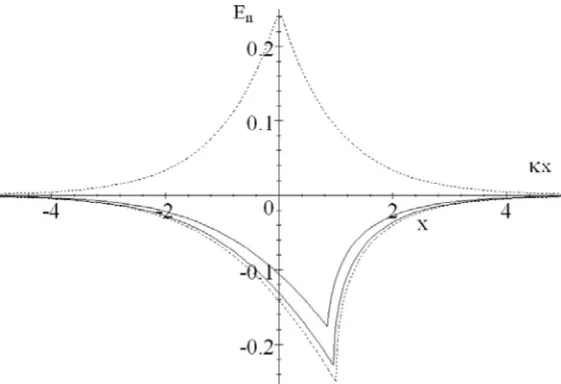
Figure 2.A plot of the normalized electric field En = 2eκE/mω2p as a function ofκxfor
different times. The upper dotted curve corresponds to ωpt = 0, the upper solid curve
corresponds toωpt=π/4, the lower solid curve corresponds toωpt= 3π/4and the lower
dotted curve corresponds toωpt=π. To complete the picture we note that the electric field
is zero everywhere forωpt=π/2as well as forωpt= 3π/2.
(see [3, (3.1)]), we then have
E(x, t) =aexp(−κ|x|) cos(ωpt).
We see from Fig. 1 that dW/dz → ∞ as z → −1/e. (Note that we use the new symbole= 2.718. . .here, whereas our previous symboledenotes the elementary charge.) Near that critical point we can write (see [3, (4.22)])W(z) =−1 +p−p2/3,
wherep2 = 2(ez+ 1), and thusdW/dz ≈e/[2(ez+ 1)]1/2. This implies thatn(x, t)
becomes infinite at this point, and this further implies from (12) thataβκ2 <1/e.
As this must hold for all times, we letβ(τ)→2e/mωp2 to obtain a condition on the amplitude of the initial electric field, namely
a <0.18
mω2
p
eκ2
≡ac. (14)
For a > ac, the solution becomes multivalued for certain values of t and xand,
hence, unphysical.
Finally, from Poisson’s equation (3) and (10), and using the relationdW/dz =
W/[z(1 +W)], one obtains
n(x, t) =n0
1 + W[aβκexp(−κ|x−x0(t)|)] cos(ωpt)
{1 +W[aβκexp(−κ|x−x0(t)|)]}[1−cos(ωpt)]
(15)
forx > x0(t). An analogous expression holds forx < x0(t). In Fig. 2 the solution
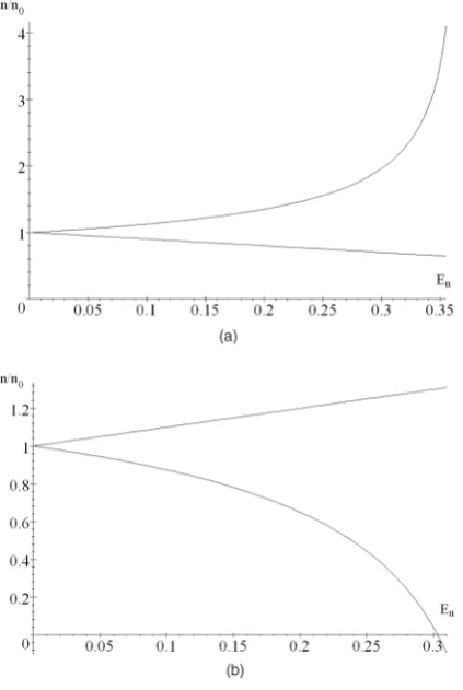
Figure 3.A plot of the maximum and minimum normalized electron densityn/n0 during
a period as a function of the normalized initial electric field amplitudeEn = 2eκ|a|/mω2p.
(a) Here a < 0, corresponding to an initial density depletion. In this case the maximum electric field amplitude is determined by the condition (14), which corresponds to the wave breaking amplitudeEn≈0.368. (b) Herea >0, corresponding to an initially positive density
perturbation. In this case the maximum allowed electric field is determined by the condition that the electron density should stay positive. The limiting casen= 0occurs for a slightly lower amplitude than in (a), withEn≈0.304.
by the condition of no wave breaking (for a negative a) or by the condition of a positive density (for a positivea), as illustrated in Fig. 3(a) and (b).
The present results significantly contribute to the existing zoo of previous solu-tions [1, 2, 5].
References
[1] Infeld, E. and Rowlands, G. 2000 Nonlinear, Waves Solitons and Chaos, 2nd edn.
Cambridge: Cambridge University Press. [2] Stenflo, L. 1996Phys. ScriptaT63, 59.
[3] Corless, R. M. et al. 1996Adv. Comput. Math.5, 329.
[4] Dubinov, A. E. and Dubinova, I. D. 2005J. Plasma Phys.71, 715.