Proceedings of the 57th Annual Meeting of the Association for Computational Linguistics, pages 4135–4145 4135
Bayes Test of Precision, Recall, and F1
Measure for Comparison of Two
Natural Language Processing Models
Ruibo Wang
School of Modern Education Technology Shanxi University
Taiyuan, China, 030006
Jihong Li School of Software
Shanxi University Taiyuan, China, 030006
Abstract
Direct comparison on point estimation of the precision (P), recall (R), and F1measure of
t-wo natural language processing (NLP) models on a common test corpus is unreasonable and results in less replicable conclusions due to a lack of a statistical test. However, the exist-ingt-tests in cross-validation (CV) for model comparison are inappropriate because the dis-tributions of P, R, F1are skewed and an
inter-val estimation of P, R, and F1based on at-test
may exceed [0,1]. In this study, we propose to use a block-regularized3×2CV (3×2BCV) in model comparison because it could regular-ize the difference in certain frequency distri-butions over linguistic units between training and validation sets and yield stable estimators of P, R, and F1. On the basis of the 3 ×2
BCV, we calibrate the posterior distributions of P, R, and F1 and derive an accurate
inter-val estimation of P, R, and F1. Furthermore,
we formulate the comparison into a hypothe-sis testing problem and propose a novel Bayes test. The test could directly compute the prob-abilities of the hypotheses on the basis of the posterior distributions and provide more infor-mative decisions than the existing significance
t-tests. Three experiments with regard to NLP chunking tasks are conducted, and the results illustrate the validity of the Bayes test.
1 Introduction
The comparison of two models is a key step in natural language processing (NLP) with the preci-sion (P), recall (R), and F1 measures. The
com-parison could be described as follows: For two NLP models on a given text corpus, which model produces a higher performance system with a rel-atively high probability? The direct comparison with a point estimation of P, R, and F1 on a test
corpus is unscientific from a statistical perspective and usually leads to less replicable results (Dror
et al.,2017). In reality, the comparison generally could be formalized with a statistical hypothesis testing, and many prominent tests, such as K-fold cross-validated (CV)t-test (Daelemans and Hoste,
2002),5×2CVt-test andF-test (Dietterich,1998;
Alpaydin,1999), and block-regularized3×2CV (3×2BCV)t-test (Wang et al.,2014), have been conducted. However, the distributions of P, R, and F1are skewed (Wang et al.,2015) and take values
in [0, 1], but an interval estimation of P, R, and F1
based on at-test may exceed [0,1].
In this study, we introduce a Bayes test that is more informative than the previous prominent nul-l hypothesis significance testing (NHST) methods in NLP (Dror et al., 2018). The test consists of three main components: (1) a3×2BCV (Li et al.,
2009;Wang et al.,2014) that provides an optimal partition of corpus and three repetitions of two-fold CV; (2) calibrated posterior distributions and accurate credible intervals (CIs) of P, R, and F1
in-stead of a normal approximation; and (3) a Bayes test of P, R, and F1that provides the probability of
which model outperforms the other.
When partitioning the corpus, certain frequen-cy distributions over linguistic units of the training set should be consistent with that of the validation set. Therefore, partitioning a corpus into two equal parts and conducting a two-fold CV are reasonable for model comparison. In fact, a3×2BCV is a specific version of an m ×2 BCV (Wang et al.,
2017a) that possesses three repetitions of two-fold CV. The three repetitions are regularized with cer-tain conditions, such as the frequency distribution of the named entity types in a named entity recog-nition (NER) task, to reduce the unintentional in-troduced difference in the frequency distributions between the training and validation sets due to the random partitioning of a corpus and to make the comparison more reliable. Particularly, them×2
pos-sesses a minimum variance, which ensures that the tests on the 3×2 BCV have higher powers and replicabilities (Wang et al.,2014,2017b).
Actually, atdistribution is inappropriate for P, R, and F1 (Yeh, 2000). Wang et al. (2015) have
obtained a posterior distribution and a CI of F1 in
a3×2BCV, but the distribution did not consider the correlations in the3×2BCV estimators, which makes the distribution inaccurate and improper in the comparison.
In this study, accurate posterior distributions and CIs of P, R, and F1 on the 3× 2 BCV are
obtained, and a Bayes test is introduced to com-pare two NLP models. The Bayes test provides the probabilities of the hypotheses in the comparison, which is more informative and reasonable than the conventional NHST. Finally, three experiments in NLP chunking tasks are used to show the validity of the Bayes test.
2 3×2BCV Posterior Distributions of P, R, and F1 of an NLP Model
AssumeDnis a text corpus, wherenis the count
of labeled instances inDn. For example,nis the
count of sentences in an NER corpus.
When computing the P, R, and F1 of an NLP
model, Dn is usually divided into two parts with
a partition (S, T) in a hold-out (HO) validation, containing a training setS, a validation setT, and Dn = S ∪ T. Assume their sizes are |S| = |T| = n/2. The confusion matrix onT isM = (TP,FP,FN,TN), where TP, FP, FN, and TN s-tand for true positive, false positive, false negative, and true negative, respectively. From these counts, one can compute the P, R and F1:
P= TP
TP+FP,R= TP
TP+FN,F1 =
2PR P+R. (1)
Goutte and Gaussier(2005) provided the natu-ral probabilistic interpretations of P and R. Specif-ically,Mfollows a multinomial distribution with parametersπ = (πT P, πF P, πF N, πT N)such that
πT P +πF P +πF N +πT N = 1. Then, P and R
estimate the following probabilities:
p=P(l=+|z=+), r=P(z=+|l=+), (2)
wherelandzrepresent the true and predicted la-bels and + indicates a positive label. Correspond-ingly, F1estimatesf1 = 2pr/(p+r).
Letn+denote the count of positive
observation-s inDn. Let(S, T)be a partition in3×2BCV, and
the count of positive observations inT satisfies
TP+FN=n+/2. (3)
2.1 Posterior Distributions of P, R, and F1 in an HO Validation
Property 2 in (Goutte and Gaussier,2005) shows that TP|TP+FN follows a binomial distribution with parameters ofn+/2andr. Then,
Var[R] =Var
[
2
n+
TP
]
= 2r(1−r)
n+
, (4)
where Var[·]is obtained overDn. The proof of Eq.
(4) is given in the supplemental material.
Assumerfollows a beta prior distribution, that is, r ∼ Be(λ, λ), and the posterior distribution ofr isr|M ∼ Be(TP+λ,FN+λ)(Goutte and Gaussier, 2005). When λ = 1, P(r|M) has a mode:
mode[r|M] =R. (5)
Similarly, assume p ∼ Be(λ, λ), andp|M ∼ Be(TP+λ,FP+λ), and its mode is
mode[p|M] =P. (6)
On the basis of the posterior distributions of P and R,Wang et al.(2015) proved that the posterior distribution of F1is
P(f1=t|M) =
2a(1−t)a−1(2−t)−a−btb−1 B(a, b) ,
(7) where B(·,·) is a beta function with parameters a=FP+FN+ 2λandb=TP+λ.
2.2 3×2BCV
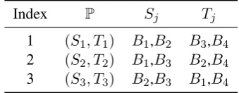
Let P = {(Sj, Tj)}3j=1 denote a partition set of
a 3 ×2 BCV with regularization conditions of
|Sj|=|Tj|and|Sj∩Sj′| ≈n/4forj̸=j′. Each
partition(Sj, Tj)corresponds to a two-fold CV.P
can be constructed with two steps: (a) Divide a text corpus Dn into four equal-sized sub-blocks,
denoted as Bi, i = 1,2,3,4. (b) Take two
sub-blocks as a training set in turn and the other two as a validation set. Table1shows the partition setP.
2.3 3×2BCV Posterior Distributions of P, R, and F1
Let M = {M(j)}3
j=1 = {(M (j)
1 ,M
(j) 2 )}3j=1
be a collection of confusion matrices in a 3×2
Index P Sj Tj
1 (S1, T1) B1,B2 B3,B4
2 (S2, T2) B1,B3 B2,B4
[image:3.595.95.265.63.129.2]3 (S3, T3) B2,B3 B1,B4
Table 1: Partition set of3×2BCV.
training set Sj and the validation setTj in thej
-th two-fold CV, and M(2j) uses Tj as the
train-ing set andSj as the validation set. LetM
(j)
k =
(TP(kj),FP(kj),FN(kj),TN(kj)).
Here, we aim to infer the posterior distributions P(p|M),P(r|M), andP(f1|M).
Conditioned onM, the micro-averaged values of P, R, and F1are
P3×2 =
1 3
∑3
j=1 12 ∑2
k=1TP (j)
k
1 3
∑3
j=112 ∑2
k=1(TP (j)
k +FP
(j)
k )
, (8)
R3×2 =
1 3
∑3
j=1 12 ∑2
k=1TP (j)
k 1 3 ∑3 j=1 1 2 ∑2
k=1(TP (j)
k +FN
(j)
k )
, (9)
F1,3×2 =
2P3×2R3×2
P3×2+R3×2
. (10)
We first investigate the posterior distribution of R, P(r|M). Considering that TPk(j) +FN(kj) =
n+/2is a constant (Eq. (3)) unrelated tojandk,
R3×2is rewritten as
R3×2=
1 3
3 ∑
j=1
R(j)= 1 6 3 ∑ j=1 2 ∑ k=1
R(kj), (11)
where
R(kj)= TP
(j)
k
TP(kj)+FN(kj)
, (12)
R(j)=
1 2
∑2
k=1TP (j)
k
1 2
∑2
k=1(TP (j)
k +FN
(j)
k )
. (13)
Thus, the variance of R3×2 is
Var[R3×2] =
1 +ρ1+ 4ρ2
3n+
r(1−r). (14)
The proof of Eq. (14) is given in AppendixA.ρ1
andρ2are two correlation coefficients between the
point HO estimators in R3×2. The definitions ofρ1
andρ2are as follows:
• Defineσ=Var
[
R(kj)
]
. According to Eq. (4), we obtainσ= 2r(1−r)/n+.
• ρ1 =Cov [
R(1j),R(2j)
]
/σis the correlation of two HO estimators in R(j)in a two-fold CV.
• ρ2 = Cov [
R(kj),R(kj′′)
]
/σ is the correlation of two HO estimators of R in different two-fold CVs, wherej ̸=j′andk, k′ = 1,2. However, the six confusion matrices inMare correlated because the three partitions are per-formed on a single text corpus and the training sets contain overlapping samples. Therefore, the like-lihood p(M|r) ̸= ∏3j=1∏2k=1p(M(kj)|r). The correlation prevents us to derive a closed form of p(r|M), which is the main challenge in this study. To overcome the challenge, aneffective confu-sion matrixMe= (TPe,FPe,FNe,TNe)is
intro-duced to measure how many independent obser-vationsMis equivalent to. Furthermore, we have r|Me∼Be(TPe+λ,FNe+λ), and the variance
of R3×2can be rewritten as
Var[R3×2] =
r(1−r)
TPe+FNe
. (15)
Comparing Eqs. (14) and (15), we obtain
TPe+FNe =
3n+
1 +ρ1+ 4ρ2
= ∑3 j=1 ∑2 k=1 (
TP(kj)+FN(kj)
)
1 +ρ1+ 4ρ2
. (16)
According to Eq. (5), we obtain
mode[r|M] = TPe
TPe+FNe
=R3×2. (17)
On the basis of Eqs. (9), (16), and (17), TPeand
FNeare expressed as
TPe=
1 1 +ρ1+ 4ρ2
3 ∑ j=1 2 ∑ k=1
TP(kj), (18)
FNe=
1 1 +ρ1+ 4ρ2
3 ∑ j=1 2 ∑ k=1
FN(kj). (19)
According to Eq. (6), we obtain
mode[p|M] = TPe
TPe+FPe
=P3×2. (20)
On the basis of Eqs. (8), (18) and (20), FPeis
FPe=
1 1 +ρ1+ 4ρ2
3 ∑ j=1 2 ∑ k=1
FP(kj). (21)
Obviously, TPe, FPe, and FNecontain unknown
• When∑ ρ1 = ρ2 = 0, TPe =
3
j=1 ∑2
k=1TP (j)
k . FNe and FPe have
sim-ilar forms. These forms indicate that the pos-terior distribution of r|M is equivalent to that on six independent text corpora.
• Whenρ1 = ρ2 = 1, TPe, FPe, and FNeare
equal to the average values of all TPs, FPs, and FNs inM, respectively. In reality, this situation indicates that the posterior distribu-tions based on3×2BCV are similar to the posterior distributions on an HO validation. Repetitions have no evident contribution to the posteriors.
In fact, R could be considered as a variant of the generalization error that takes the expectation of zero-one loss on merely positive observation-s. Correlationsρ1 andρ2 in3×2BCV estimator
of the generalization error have been investigated (Wang et al.,2014,2017a). The works empirical-ly indicate0 ≤ ρ1 ≤ 1/2and1/4 ≤ ρ2 ≤ 1/2,
which are also applicable for the correlations in R3×2. To eliminate unknown ρ1 and ρ2 in TPe,
FNe, and FPe, we take their averages over the
range of 0 ≤ ρ1 ≤ 1/2 and1/4 ≤ ρ2 ≤ 1/2
regardless of the model used. Hence,
TPe ≈ 8
∫0.5
0.25 ∫0.5
0 ∑3
j=1 ∑2
k=1TP (j)
k
1 +ρ1+ 4ρ2
dρ1dρ2
≈ 0.3688
3 ∑
j=1 2 ∑
k=1
TP(kj). (22)
Similarly, we obtain
FNe≈0.3688
3 ∑
j=1 2 ∑
k=1
FN(kj), (23)
FPe≈0.3688
3 ∑
j=1 2 ∑
k=1
FP(kj). (24)
In sum,3×2BCV posterior distributions of P, R and F1are
P(p=t|M) = t
TPe+λ(1−t)FPe+λ B(TPe+λ,FPe+λ)
, (25)
P(r =t|M) = t
TPe+λ(1−t)FNe+λ B(TPe+λ,FNe+λ)
, (26)
P(f1 =t|M) =
2¯a(1−t)¯a−1(2−t)−¯a−¯bt¯b−1
B(¯a,¯b) ,
(27)
whereB(·,·)is a beta function with parameters of
¯
a = FPe+FNe+ 2λand¯b = TPe+λ. In this
study,λ= 1is used.
2.4 CIs of P, R, and F1Based on3×2BCV
On the basis of the3×2BCV posterior distribu-tions of P, R, and F1, their corresponding CIs could
be derived. The CI of P with a probability1−αis
CIp= [ Beα
2(TPe+λ,FPe+λ),
Be1−α2(TPe+λ,FPe+λ)].(28)
The CI of R is
CIr = [ Beα
2(TPe+λ,FNe+λ), Be1−α
2(TPe+λ,FNe+λ)].(29) The CI of F1is
CIf1 =
[
2 2 +Be′1−α
2 , 2
2 +Be′α 2
]
, (30)
whereBe′α is the αquantile of a beta-prime dis-tribution with parameters of FPe+FNe+ 2λand
TPe+λ.
The above CIs are more accurate than the previ-ously proposed CIs (Wang et al.,2015;Wang and Li, 2016) because the parameters in the posterior distributions are corrected via the correlations in the3×2BCV estimator. Take F1as an example.
A different CI of F1based on3×2BCV is given
in (Wang et al., 2015), which employs the aver-aged values of FPs, FNs, and TPs inM. Their CI is a special case of Eq. (30) with ρ1 = ρ2 = 1.
Their CI is more conservative, that is, the actual degree of credibility (DOC) is larger than the nom-inal probability (1−α). Nevertheless, our CI is more accurate because it could relieve the conser-vativity, which is shown in the following example.
Example: Consider a similar simulation in (Wang et al.,2015), which uses a classification da-ta set with two classes. A sample isZ = (X, Y)
whereP(Y = 1) =P(Y = 0) = 12, andX|Y = 0 ∼ N(µ0,Σ0), X|Y = 1 ∼ N(µ1,Σ1). Take
µ0 = (0,0),µ1 = (0.5,0.5), andΣ0 = Σ1 =I2.
The data set size isn = 600andα = 0.05. With a logistic regression algorithm, the DOC and in-terval length (IL) of their CI are99.6%and0.117. However, the DOC and IL of our CI are 94.5%
3 Bayes Test for Comparison of Two NLP Models
For an NLP task, assume A is a state-of-the-art model usingDn. When a modelBis crafted out, it
is indispensable to compare it withAto document whetherBperformssignificantlybetter thanAby employing the following hypotheses:
H0 :νB −νA ≤0 v.s. H1 :νB−νA >0, (31)
where νA and νB are the evaluation metrics of models A and B. In this study, P, R and F1 are
considered.
We address Problem (31) with a Bayes test (Casella and Berger, 2002), which is different to previous NHST studies (Dietterich, 1998; Alpay-din,1999;Yildiz,2013). A Bayes test could avoid many shortcomings of NHST reasoning, such as the egregious logic error inp-value. Moreover, a Bayes test could directly compute the probabili-ties of the hypotheses, which help users to make a more reasonable decision. Thus, a Bayes test is increasingly preferred and recommended recently as an advanced tool to analyze the experimental results (Benavoli et al.,2016).
In this study, we propose a Bayes test that uses the3×2BCV posterior distributions of P, R, and F1to calculate the probabilities of hypotheses,
de-noted asP(H0)andP(H1). Then, the test infers
a decision with the heuristic rules: AcceptH0 iff
P(H0)≥P(H1); otherwise acceptH1.
Before elaborating the Bayes test, several nec-essary denotations are introduced: theMof mod-elAisMA; the TPe, FNe, and FPe of modelA
are TPe,A, FNe,A, and FPe,A, respectively. Thep,
r, andf1 ofA are pA, rA, and f1,A, respective-ly. The denotations of B are defined in a simi-lar manner. Letν denote a user-defined metric in
{P,R,F1}. For example, if user assign R toν, then
rA andrB are compared.
The key point to perform a Bayes test on Prob-lem (31) is to tackle the distribution of the differ-ence of νA −νB. However, no explicit form of the distribution exists. Thus, we estimate it using the Monte-Carlo simulation. Take R as an exam-ple. Conditioned onMA andMB, assumingrA is independent ofrB, we wish to evaluate the prob-abilityp(rA−rB ≤0MA,MB), that is,
∫1
0 ∫1
0
I(rA−rB ≤0)P(rA|MA)
·P(rB|MB)drAdrB, (32)
where I(·) is the indicator function that has val-ue oneiff the enclosed condition is true and zero otherwise. Considering that no close form of Eq. (32) exists, we have to evaluate it using Monte-Carlo simulation: (a) Sample a large number of observations from P(rA|MA) and P(rB|MB), and denote them as{si,A}Li=1 and{si,B}Li=1; (b)
approximate Eq. (32) with the empirical propor-tion:
1
L
L
∑
i=1
I(si,A−si,B ≤0), (33)
whereL= 1,000,000is used.
Input: Text corpus,Dn; NLP models,AandB;
Evaluation metric,ν;
Output: Probabilities of the hypotheses and a decision between “AcceptH0” and “AcceptH1”; 1 ConstructPonDnaccording to Table1;
2 Train and validate modelsAandBonP, and summarize the results asMAandMB, respectively; 3 Apply Eqs. (22), (23) and (24) onMA andMBto get
(TPe,A,FNe,A,FPe,A)and(TPe,B,FNe,B,FPe,B);
4 ifνisPthen
5 P(νA|MA)←use Eq. (25) on TPe,Aand FPe,A;
6 P(νB|MB)←use Eq. (25) on TPe,Band FPe,B;
7 end
8 else ifνisRthen
9 P(νA|MA)←use Eq. (26) on TPe,Aand FNe,A;
10 P(νB|MB)←use Eq. (26) on TPe,Band FNe,B;
11 end
12 else ifνisF1then
13 P(νA|MA)←use Eq. (27) on TPe,A, FPe,Aand
FNe,A;
14 P(νB|MB)←use Eq. (27) on TPe,B, FPe,Band
FNe,B;
15 end
16 ApproximateP(νA−νB≤0MA,MB)with Monte-Carlo simulation (refer to Eq. (33)); 17 P(H0)←P(νA−νB ≤0MA,MB); 18 P(H1)←1−P(νA−νB ≤0MA,MB); 19 ifP(H0)≥P(H1)then
20 Return (P(H0),P(H1), “AcceptH0”); 21 end
22 else
23 Return (P(H0),P(H1), “AcceptH1”); 24 end
Algorithm 1:A Bayes test for comparing P, R and F1of two NLP models.
On the basis of the above analysis, the sketch of Bayes test is shown in Algorithm1. The algo-rithm performs hypothesis testing procedures for P, R, and F1 according to the specific value ofν.
the Bayes test helps users to investigate the differ-ence ofAandBwith different perspectives and in a fine-grained manner.
Bayes test and NHST are two different types of significant tests from two philosophies: Bayesian and frequentist inferences. When the distribution of an evaluation metric is available, the Bayes test may provide more informative inferences and con-clusions than the NHST. Until now, no mature and fair criterion to compare Bayes test and NHST ex-ists. Therefore, in this study, an objective compar-ison between them is not provided. Instead, we show three experiments to illustrate the validity of the Bayes test.
4 Experiments and Analysis
The experiments concentrate on chunking tasks1. Chunking is an important task in NLP, which in-cludes Chinese word segmentation (CWS) and N-ER. A chunking task could be formulated into a sequence labeling problem and addressed by em-ploying a tag set, such as IOB2 and IOBES ( Ku-do and Matsumoto,2001;Shen and Sarkar,2005), and a widely used algorithm, such as conditional random fields (CRFs) (Lafferty et al., 2001) and LSTM (Hochreiter and Schmidhuber,1997; Lam-ple et al.,2016).
In this section, we perform the Bayes test on NLP chunking models with different tag sets to answer a question: could a fine-grained tag set im-prove the performance of a chunking model?
A chunking model is usually evaluated in terms of the metrics of P, R, and F1. When computing
them, TP indicates the count of correctly predict-ed chunks, FN is the count of golden chunks that are incorrectly predicted, and FP is the count of predicted chunks that are not correct.
Three different chunking tasks are considered:
CWS task: Identify a reasonable word se-quence in a raw sentence. A word is regarded as a chunk, and every character in the sentence enter-s into a chunk. Bakeoff-2005 CWS PKU training corpus is used asDn.
NER task: Identify the boundaries of all N-ER chunks without recognizing their types. CoN-LL 2003 English NER training set is used as Dn, which contains four types of NER, namely,
“PER”, “LOC”, “ORG”, and “MISC”. Word is
1The code for the experiments in this paper is found on:
https://github.com/RamboWANG/acl2019
used as a tagging unit, and considerable out-of-chunk words exist.
ORG task: Identify only “ORG” entities. The corpus is the same to the NER task. The count of “ORG” chunks is remarkably smaller than the count of NER chunks in the NER task, and the out-of-chunk words dominate the corpus.
In the above three tasks, CRFs are used as the sequence labeling algorithm. Other algorithms will be studied in future research.
4.1 CWS Task: “BMES” Versus
“BB2B3MES”
The CWS task is formulated into a sequence la-beling problem at character level. Two different tag sets of “BMES” and “BB2B3MES” are
con-sidered, which correspond to modelsAandB, re-spectively. “BB2B3MES” is a fine-grained set that
introduces two additional tags of “B2” and “B3”
on the basis of “BMES”. Zhao et al. (2006) illus-trated that model B improves A without investi-gating the significance, which is performed here.
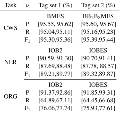
Task ν Tag set 1 (%) Tag set 2 (%)
CWS
BMES BB2B3MES
P [95.55, 95.62] [95.60, 95.67] R [95.04,95.11] [95.16,95.23] F1 [95.30,95.36] [95.39,95.44]
NER
IOB2 IOBES
P [90.59, 91.30] [90.70,91.41] R [87.69,88.48] [87.78, 88.57] F1 [89.21,89.77] [89.32,89.87]
ORG
IOB2 IOBES
[image:6.595.313.520.378.574.2]P [91.37,92.86] [91.85,93.31] R [64.89,67.11] [64.45,66.68] F1 [76.06,77.74] [75.93,77.61]
Table 2: CIs of the three tasks (α= 0.05).
ν P(H0) P(H1) Decision
P 0.024 0.976 AcceptH1
R 0.001 0.999 AcceptH1
[image:6.595.331.502.624.689.2]F1 0.001 0.999 AcceptH1
Table 3: Decisions of the Bayes test in the CWS task.
0.955 0.956 0.957
0 500 1000 1500 2000
P posterior
0.950 0.951 0.952
0 500 1000 1500 2000
R posterior
0.953 0.954
0 1000 2000
3000 F1 posterior
[image:7.595.75.278.58.232.2]BMES (this study) BMES (Wang et al., 2015) BB2B3MES (this study) BB2B3MES (Wang et al., 2015)
Figure 1:3×2BCV posterior distributions in the CWS task.
the two CWS models are given in Figure1, and the CIs inα = 0.05are given in Table2. Each curve ranges from0.001quantile to0.999quantile. The curves in solid lines correspond to Eqs. (25), (26), and (27), which are recommended in this study.
Two observations are concluded from Figure1. First, our proposed posterior distributions, which yield more accurate CIs, are taller and thinner than those in (Wang et al.,2015). Second, the posterior distributions of the R and F1 between modelsA
andBhave smaller overlaps than those of P. The smaller overlap indicates that the additional tags of “B2” and “B3” mainly improve the R and F1of
the CWS model.
The Bayes test is performed onAandB. The probabilities of the hypotheses and decisions are given in Table 3. H1 holds in the probability of
0.98 for P, whereasH1holds in the probabilities of
approximately 1 for R and F1. Table3illustrates
that the fine-grained tag set significantly improves the CWS model, and the improvements in R and F1are larger than P.
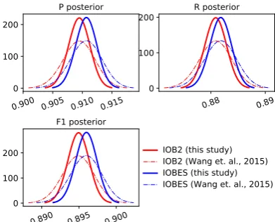
4.2 NER Task: “IOB2” Versus “IOBES”
In this task, word and POS are used as features. The unigram, bigram, and trigram of word and POS are included in the feature template. The window size of each type of feature is set to [-2,2]. “IOBES” in model B is a fine-grained tag set, which adds tags “E” and “S” to “IOB2” inA. Posterior distributions of P, R, and F1 of
mod-elsAandB are given in Figure2. The posterior distributions of the two models have large over-laps, which indicate that the improvement in B
0.900 0.905 0.910 0.915
0 100 200
P posterior
0.88 0.89
0 100
200 R posterior
0.890 0.895 0.900
0 100 200
F1 posterior
IOB2 (this study) IOB2 (Wang et. al., 2015) IOBES (this study) IOBES (Wang et. al., 2015)
Figure 2:3×2BCV posterior distributions in the NER task.
is not evident. Corresponding CIs are given in Table 2. The CIs of the two models have also large overlaps, indicating the insignificant differ-ences between the two models. Table 4 presents the decisions of the Bayes test, which are iden-tical on the three metrics, that is, “Accept H1”.
However, the improvement is not remarkable be-cause P(H1) are lower than 0.8. Moreover, the
fine-grained tag set, “IOBES,” exerts more effort to improve P than R becauseP(H1) = 0.68for P
is larger thanP(H1) = 0.63for R.
ν P(H0) P(H1) Decision
P 0.321 0.679 AcceptH1
R 0.372 0.628 AcceptH1
[image:7.595.311.507.65.223.2]F1 0.300 0.700 AcceptH1
Table 4: Decisions of the Bayes test in the NER task.
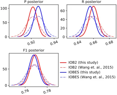
4.3 ORG Task: “IOB2” Versus “IOBES”
In this task, the settings of features are the same with the NER task. However, the distributions of tags become more skewed than those of the NER task, that is, tag “O” possesses a larger proportion. Thus, the decisions of the Bayes test are remark-ably different. Specifically, the posterior distribu-tions of P, R, and F1 are given in Figure3, which
indicate that the improvement inBis not evident. Surprisingly, for R and F1, the posterior
distribu-tion ofBshifts to the left of that ofA, which illus-trates the fine-grained tag set, namely, “IOBES,” deteriorates R and F1. A possible reason is the
[image:7.595.329.502.462.527.2]ν P(H0) P(H1) Decision
P 0.191 0.809 AcceptH1
R 0.706 0.294 AcceptH0
[image:8.595.95.267.64.129.2]F1 0.587 0.413 AcceptH0
Table 5: Decisions of the Bayes test in the ORG task.
0.92 0.94
0 50 100
P posterior
0.64 0.66 0.68
0 20 40 60
R posterior
0.76 0.78
0 50
F1 posterior
IOB2 (this study) IOB2 (Wang et. al., 2015) IOBES (this study) IOBES (Wang et. al., 2015)
Figure 3:3×2BCV posterior distributions in the ORG task.
more skewed proportions of tags than “IOB2.” The decisions of the Bayes test are given in Ta-ble 5. The probability of the improvement to P exceeds 0.8, that is,P(H1) = 0.81. However, the
fine-grained tag set harms R and F1 in a sense of
P(H0) = 0.71for R andP(H0) = 0.59for F1.
The above three tasks illustrate the validity of the Bayes test, which provide accurate CIs of P, R, and F1 and the estimation of P(H0)andP(H1).
The results are more informative for interpreta-tions and help to make a reliable decision.
5 Related Work
Over the last few past decades, many studies have contributed to validate whether the stan-dard significant tests are adequate for comparing NLP models (Gillick and Cox, 1989;Yeh, 2000;
Daelemans and Hoste, 2002; Koehn, 2004; Rie-zler and Maxwell, 2005;Berg-Kirkpatrick et al.,
2012;Søgaard,2013;Søgaard et al.,2014;N´ev´eol et al.,2016;Dror et al.,2017,2018). These stud-ies observed that standard tests tend to infer invalid comparison conclusions. Two important questions arise from the observations: 1) How to correct-ly perform CV for NLP model comparison? 2) What are the distributions of the common
evalua-tion metrics in NLP, such as P, R, and F1?
The first question could refer to many stud-ies in machine learning, which investigated vari-ous CV methods in algorithm comparison, includ-ing repeated learninclud-ing-testinclud-ing (Nadeau and Ben-gio,2003;Wang et al.,2019), K-fold CV (Kohavi et al.,1995;Rodr´ıguez et al.,2010,2013; Moreno-Torres et al., 2012), 5×2CV (Dietterich, 1998;
Alpaydin, 1999;Yildiz, 2013), andm ×2 BCV (Wang et al., 2014, 2015, 2017a,b). In these s-tudies, m ×2 BCV might be a better option for comparing NLP models because it leads to stable estimation of evaluation metrics and the m ×2
BCV tests possesses higher powers and replica-bilities (Wang et al., 2014, 2017b). Moreover, on a text corpus, certain frequency distributions over linguistic units between training and valida-tion sets in two-fold CV intuitively possess small-er divsmall-ergence than those in five-fold or ten-fold CV. Therefore,m×2BCV should be investigated when comparing NLP models.
The second question is pioneered in the work of (Goutte and Gaussier,2005), which proved the posterior distributions of P and R in an HO val-idation. The posterior distributions make an ex-act comparison possible (Zhang and Su, 2012;
Wang and Li,2016). However, the distribution of F1 is difficult to tackle, because it is a complex
function. Zhang et al.(2015a,b, 2016) employed complicated probabilistic graphic representations and Bayesian hierarchical models to estimate and compare F1 measures. Fortunately, Wang et al.
(2015) obtained an exact close-form of posterior distribution of F1, which is a function with regard
to a beta-prime distribution. These studies pro-vided a rigorous theoretical guarantee for pursuing the3×2BCV posterior distributions of P, R, and F1.
6 Conclusions and Future Work
In this study, we obtained accurate posterior distri-butions of P, R, and F1on the basis of a3×2BCV,
[image:8.595.77.273.169.329.2](1) At-test should be avoided in a comparison of two NLP models on the basis of the precision, recall and F1measure.
(2) The3×2BCV could be preferred to evaluate the performance of an NLP model in the task of model comparison.
(3) The Bayes test on the basis of the3×2BCV could provide informative and fine-grained measures of the differences of precisions, re-calls and F1measures of two NLP models, and
the measures could help practitioners to make a reasonable decision.
In the future, we will refine the Bayes test of P, R, and F1 in anm×2BCV and provide
accu-rate interval estimation of other evaluation metrics on the basis of the confusion matrix. Obtaining the posterior distribution of an evaluation metric of a model is still a key problem in this valuable research area.
Acknowledgments
We thank the anonymous reviewers for their help-ful comments. This work is supported by the Na-tional Social Science Foundation of China under Grants no. 16BTJ034. The experiments are sup-ported by High Performance Computing System of Shanxi University. The corresponding author is Jihong Li.
References
Ethem Alpaydin. 1999. Combined5×2cv f-test for comparing supervised classification learning algo-rithms. Neural Computation, 11(8):1885–1892.
Alessio Benavoli, Giorgio Corani, Janez Demsar, and Marco Zaffalon. 2016. Time for a change: a tutorial for comparing multiple classifiers through bayesian analysis. Journal of Machine Learning Research, 18.
Taylor Berg-Kirkpatrick, David Burkett, and Dan K-lein. 2012. An empirical investigation of statistical significance in nlp. InProceedings of the 2012 Joint Conference on Empirical Methods in Natural guage Processing and Computational Natural Lan-guage Learning, pages 995–1005. Association for Computational Linguistics.
George Casella and Roger L Berger. 2002. Statistical inference, volume 2. Duxbury Pacific Grove, CA.
Walter Daelemans and V´eronique Hoste. 2002. Eval-uation of machine learning methods for natural lan-guage processing tasks. InProceedings of the Third
International Conference on Language Resources and Evaluation, pages 755–760.
Thomas G Dietterich. 1998. Approximate statistical tests for comparing supervised classification learn-ing algorithms. Neural computation, 10(7):1895– 1923.
Rotem Dror, Gili Baumer, Marina Bogomolov, and Roi Reichart. 2017. Replicability analysis for natural language processing: Testing significance with mul-tiple datasets. Transactions of the Association for Computational Linguistics, 5:471–486.
Rotem Dror, Gili Baumer, Segev Shlomov, and Roi Reichart. 2018. The hitchhikers guide to testing statistical significance in natural language process-ing. Proceedings of the 56th Annual Meeting of the Association for Computational Linguistics (Volume 1: Long Papers), pages 1383–1392. Association for Computational Linguistics.
Laurence Gillick and Stephen J Cox. 1989. Some s-tatistical issues in the comparison of speech recog-nition algorithms. In International Conference on Acoustics, Speech, and Signal Processing,, pages 532–535. IEEE.
Cyril Goutte and Eric Gaussier. 2005. A probabilistic interpretation of precision, recall and f-score, with implication for evaluation. InEuropean Conference on Information Retrieval, pages 345–359. Springer.
Sepp Hochreiter and J¨urgen Schmidhuber. 1997. Long short-term memory. Neural computation, 9(8):1735–1780.
Philipp Koehn. 2004. Statistical significance tests for machine translation evaluation. In Proceedings of the 2004 conference on empirical methods in natural language processing.
Ron Kohavi et al. 1995. A study of cross-validation and bootstrap for accuracy estimation and model s-election. In Ijcai, volume 14, pages 1137–1145. Montreal, Canada.
Taku Kudo and Yuji Matsumoto. 2001. Chunking with support vector machines. In Proceedings of the second meeting of the North American Chapter of the Association for Computational Linguistics on Language technologies, pages 1–8. Association for Computational Linguistics.
John D. Lafferty, Andrew McCallum, and Fernando C. N. Pereira. 2001. Conditional random fields: probabilistic models for segmenting and labeling se-quence data. InProceedings of the Eighteenth In-ternational Conference on Machine Learning (ICM-L 2001), Williams College, Williamstown, MA, USA, June 28 - July 1, 2001, pages 282–289.
Jihong Li, Ruibo Wang, Weilin Wang, Bo Gu, and Guochen Li. 2009. Automatic labeling of semantic role on chinese framenet using conditional random fields. InProceedings of the 2009 IEEE/WIC/ACM International Joint Conference on Web Intelligence and Intelligent Agent Technology-Volume 03, pages 259–262. IEEE Computer Society.
Jose G Moreno-Torres, Jos A Sez, and Francisco Her-rera. 2012. Study on the impact of partition-induced dataset shift onk-fold cross-validation. Neural Net-works and Learning Systems, IEEE Transactions on, 23(8):1304–1312.
Claude Nadeau and Yoshua Bengio. 2003. Inference for the generalization error. Machine Learning, 52(3):239–281.
Aur´elie N´ev´eol, Kevin Cohen, Cyril Grouin, and Aude Robert. 2016. Replicability of research in biomed-ical natural language processing: a pilot evaluation for a coding task. InProceedings of the Seventh ternational Workshop on Health Text Mining and In-formation Analysis, pages 78–84.
Stefan Riezler and John T Maxwell. 2005. On some pitfalls in automatic evaluation and significance test-ing for mt. InProceedings of the ACL workshop on intrinsic and extrinsic evaluation measures for ma-chine translation and/or summarization, pages 57– 64.
Juan D Rodr´ıguez, Aritz P´erez, and Jose A Lozano. 2010. Sensitivity analysis of k-fold cross valida-tion in predicvalida-tion error estimavalida-tion. Pattern Analy-sis and Machine Intelligence, IEEE Transactions on, 32(3):569–575.
Juan D Rodr´ıguez, Aritz P´erez, and Jose A Lozano. 2013. A general framework for the statistical analy-sis of the sources of variance for classification error estimators. Pattern Recognition, 46(3):855–864.
Hong Shen and Anoop Sarkar. 2005. Voting be-tween multiple data representations for text chunk-ing. In Conference of the Canadian Society for Computational Studies of Intelligence, pages 389– 400. Springer.
Anders Søgaard. 2013. Estimating effect size across datasets. InProceedings of the 2013 Conference of the North American Chapter of the Association for Computational Linguistics: Human Language Tech-nologies, pages 607–611.
Anders Søgaard, Anders Johannsen, Barbara Plank, Dirk Hovy, and H´ector Mart´ınez Alonso. 2014. What’s in a p-value in nlp? In Proceedings of the eighteenth conference on computational natural lan-guage learning, pages 1–10.
Ruibo Wang, Jihong Li, Xingli Yang, and Jing Yang. 2019. Block-regularized repeated learning-testing for estimating generalization error. Information Sci-ences, 477:246–264.
Ruibo Wang, Yu Wang, Jihong Li, Xingli Yang, and Jing Yang. 2017a. Block-regularizedm×2 cross-validated estimator of the generalization error. Neu-ral Computation, 29(2):519–554.
Yu Wang and Jihong Li. 2016. Credible interval-s for preciinterval-sion and recall bainterval-sed on a k-fold crointerval-sinterval-s- cross-validated beta distribution. Neural Computation, 28(8):1694–1722.
Yu Wang, Jihong Li, and Yanfang Li. 2017b. Choos-ing between two classification learnChoos-ing algorithms based on calibrated balanced5×2cross-validated f-test. Neural Processing Letters, 46(1):1–13.
Yu Wang, Jihong Li, Yanfang Li, Ruibo Wang, and X-ingli Yang. 2015. Confidence interval for f1
mea-sure of algorithm performance based on blocked 3x2 cross-validation. IEEE Transactions on Knowledge & Data Engineering, 27(3):651–659.
Yu Wang, Ruibo Wang, Huichen Jia, and Jihong Li. 2014. Blocked 3×2 cross-validated t-test for com-paring supervised classification learning algorithms.
Neural Computation, 26(1):208–235.
Alexander Yeh. 2000. More accurate tests for the s-tatistical significance of result differences. In Pro-ceedings of the 18th conference on Computation-al linguistics-Volume 2, pages 947–953. Association for Computational Linguistics.
Olcay Taner Yildiz. 2013. Omnivariate rule induc-tion using a novel pairwise statistical test. IEEE Transactions on Knowledge and Data Engineering, 25(9):2105–2118.
Dell Zhang, Jun Wang, Emine Yilmaz, Xiaoling Wang, and Yuxin Zhou. 2016. Bayesian performance com-parison of text classifiers. In Proceedings of the 39th International ACM SIGIR conference on Re-search and Development in Information Retrieval, pages 15–24. ACM.
Dell Zhang, Jun Wang, and Xiaoxue Zhao. 2015a. Es-timating the uncertainty of average f1 scores. In Proceedings of the 2015 International Conference on The Theory of Information Retrieval, pages 317– 320. ACM.
Dell Zhang, Jun Wang, Xiaoxue Zhao, and Xiaoling Wang. 2015b. A bayesian hierarchical model for comparing average f1scores. InData Mining (ICD-M), 2015 IEEE International Conference on, pages 589–598. IEEE.
Peng Zhang and Wanhua Su. 2012. Statistical infer-ence on recall, precision and average precision under random selection. InFuzzy Systems and Knowledge Discovery (FSKD), 2012 9th International Confer-ence on, pages 1348–1352. IEEE.
A Proof of Eq. (4)
According to Eqs. (1) and (3), we obtain
R= TP
TP+FN =
2TP n+
. (34)
Because TP|TP+FN follows a binomial distri-bution with parameters of n+/2 andr and TP+
FN=n+/2is a constant, we obtain
Var[TP] = n+
2 r(1−r). (35)
Based on Eq. (34), we know
Var[R] = Var[2TP
n+
] = 4
n2 +
Var[TP]
= 2r(1−r)
n+
.
B Proof of Eq. (14)
According to Eq. (11), Var[R3×2]can be
decom-posed into
Var[R3×2] =Var 1
3
3 ∑
j=1
R(j)
= 1 9
{ 3 ∑
j=1
Var
[
R(j)
]
+
3 ∑
j=1 3 ∑
j′=1
j̸=j′
Cov
[
R(j),R(j′)
] }
. (36)
Assume Var
[
R(j)
]
doesn’t depend on the
par-ticular realization ofPj, then Var
[
R(j)
]
for all j are identical. Furthermore, since the number of overlapping samples between the two training sets inPj andPj′equals ton/4withj̸=j′, we could
reasonably assume Cov
[
R(j),R(j′)
]
for allj̸=j′ are identical and independent to j andj′. Thus, we obtain
Var[R3×2] =
1 3
{
Var
[
R(j)
]
+2Cov
[
R(j),R(j′)
] }
.(37)
Since R(j) = (R1(j) + R(2j))/2, assume Var
[
R(1j)
]
=Var
[
R(2j)
]
, we have
Var
[
R(j)
]
=Var
[
1 2(R
(j)
1 +R
(j) 2 )
]
= 1 2
{
Var
[
R(kj)
]
+Cov
[
R(kj),R(kj′)
] }
, (38)
wherek̸= k′. Furthermore, according to Eq. (4) and the definition ofρ1, we obtain
Var
[
R(kj)
]
= 2r(1−r)/n+, (39)
Cov
[
R(kj),R(kj′)
]
= 2ρ1r(1−r)/n+. (40)
Substituting Eqs. (39) and (40) into Eq. (38), we obtain
Var
[
R(j)
]
= 1 +ρ1
n+
r(1−r). (41)
Similarly, assume Cov
[
R(kj),R(kj′′)
]
doesn’t
de-pend onkandk′, then
Cov
[
R(j),R(j′)
]
=Cov
[
R(kj),R(kj′′)
]
, (42)
wherek, k′ = 1,2. According to the definition of ρ2, we obtain
Cov
[
R(j),R(j′)
]
= 2ρ2
n+
r(1−r). (43)
Substituting Eqs. (41) and (43) into Eq. (37), we obtain
Var[R3×2] =
1 +ρ1+ 4ρ2
3n+
r(1−r).