Munich Personal RePEc Archive
Do reserve requirements reduce the risk
of bank failure?
Glocker, Christian
Austrian Institute of Economic Research
August 2019
Online at
https://mpra.ub.uni-muenchen.de/95634/
FAILURE?
CHRISTIAN GLOCKER
Abstract. There is an increasing literature proposing reserve requirements for financial stability. This study assesses their effects on the probability of bank failure and compares them to those of capital requirements. To this purpose a banking model is considered that is subject to legal reserve requirements. In general, higher reserve requirements promote risk-taking as either borrowers or banks have an incentive to choose riskier assets, so banks’ probability of failure rises. Borrowers’ moral hazard problem augments the adverse effects. They are mitigated when allowing for imperfectly correlated loan-default as higher interest revenues from non-defaulting loans curb losses from defaulting loans.
JELcodes: E43, E58, G21, G28
Key words: reserve requirements, liquidity regulation, capital requirements, bank failure, default correlation
This version: August 2019 – Comments are welcome.
C. Glocker: Austrian Institute of Economic Research, Arsenal Objekt 20, 1030 Vienna, Austria. Phone: +43 (0) 1 789 26 01-303, E-mail: [email protected].
1. Introduction
At the centre of the discussion on financial stability is the question of how much
capital and reserves banks should be required to hold. A system with a buffer too
small might be crisis-prone and in need of regular bail-outs. On the other hand, too
much might render unprofitable large parts of the banking business. In this context,
capital requirements are one of the most important instruments and address banks’
balance sheets directly. Yet they comprise just another of two distinct well-known
regulatory instruments. Reserve requirements have traditionally been used, though
not necessarily with a sole financial stability objective.
Both requirements concern the composition of banks’ balance sheets. Changing
one of them simply has a mirror image effect as the other, since both are defined as
ratios between asset and liability categories. For both requirements, an increase is
associated with a balance sheet tightening. The similarity of the effects of changes in
either of the two regulatory requirements on banks’ balance sheets motivates a joint
assessment of their effects. The effects of capital requirements on lending rates and
financial stability have been analysed extensively in the literature (see Gambacorta
and Karmakar, 2018; Repullo and Suarez, 2013; Covas and Fujita, 2010; VanHoose,
2007, for an overview). In contrast, reserve requirements have not yet been assessed
in this context. Against this background, the aim of this study is to evaluate the
effects of reserve requirements on the probability of bank failure.
As reserve requirements are the key element in characterising a fractional banking
system, they have hence been analysed from the perspective of an instrument for
monetary policy for a long time (see for instance Day, 1986; Vernon, 1990; Davis
and Toma, 1995; Haslag and Young, 1998; Faig and Gagnon, 2008; Carpenter and
Demiralp, 2012; Dutkowsky and VanHoose, 2013; Hendrickson, 2017; Armenter and
Lester, 2017). The experience of emerging market economies has induced a change
in the perception of the usefulness of reserve requirements (Hoffmann and L¨offler,
2014). The recent literature highlights the importance of reserve requirements as
a means to foster financial stability, which is motivated by the fact that reserve
requirements operate directly on the narrow credit channel defined by the supply
reaction of bank credit to a change in available funds (Calomiris and Kahn, 1991;
A series of recent theoretical papers has assessed the ability of reserve
require-ments to promote financial stability for which most of them rely on dynamic
sto-chastic general equilibrium (DSGE) models. In this context, Glocker and Towbin
(2012); Mimir et al. (2013); Ireland (2014); De Carvalho et al. (2013); Bustamante
and Hamann (2015); Primus (2017); Ag´enor et al. (2018); Adrian and Boyarchenko
(2018); Imhof et al. (2018); Yang and Yi (2019); Mimir and Sunel (2019); Silva
Vin-hado and Divino (2019), among others, find that reserve (or liquidity) requirements
have the ability to contain the degree of procyclicality of the financial system and by
this to foster financial stability. The argument is that reserve requirements can serve
as a countercyclical tool to manage the credit cycle in a broad context, limiting the
excessive leverage of borrowers in the upswing and operating as a liquidity buffer in
the downswing.
The empirical literature generally confirms these findings. In particular, Montoro
and Moreno (2011); Tovar et al. (2012); Glocker and Towbin (2015); Fung´a˘cov´a et
al. (2016); Becker et al. (2017); Crespo Cuaresma et al. (2019); Dassatti Camors et
al. (2019) provide empirical evidence highlighting that spikes in reserve requirements
are likely to exert a downward pressure on loans and upward pressure on lending
rates. Kashyap and Stein (2012) stress the importance of reserve requirement
poli-cies to augment the possibilities of central banks to achieve financial stability. They
argue that reserve requirements could be considered as a Pigouvian tax used to
in-ternalise the externalities generated by a high short-term debt exposure of financial
intermediaries.1
Common to this literature is (i) their perception of reserve requirements as an
adequate instrument for financial stability purposes, (ii) their focus on the
macroe-conomy and (iii) the absence of an explicit measure for financial stability. In line with
most studies, Barroso et al. (2017), Andries et al. (2018) and Alper et al. (2018) find
that reserve requirements affect credit growth, most importantly, they document an
effect on risk-taking by banks. They stress that banks that are more affected by
countercyclical reserve requirements avoid riskier firms, showing that higher reserve
requirements are likely to mitigate bank risk-taking. However, in contrast, the
re-sults of Ely et al. (2019), Dassatti Camors et al. (2019) and Jim´enez et al. (2017)
point towards the opposite. They document a “search-for-yield” effect (that is, a
positive risk-taking response) to the tightening of reserve requirements.2
This raises
questions about the (i) presence of a risk-shifting effect and (ii) the ability of reserve
requirements to promote financial stability.
We analyse under which circumstances reserve requirements promote financial
stability, which we assess by means of the probability of bank failure. To that
purpose, we consider a banking model of Cournot competition within a perfectly
competitive market for loans. Banks have zero intermediation costs, are funded
with fully insured deposits and equity capital. We introduce a central authority
which, apart from the interest rate, sets legal reserve requirements. We extend the
model along two dimensions. The first dimension addresses the risk environment.
The differing results found for the effects of capital requirements on bank risk-taking
are due to different modelling approaches (Hakenes and Schnabel, 2011). In the first
type of models, banks solve aportfolio problem. They hold a portfolio of projects and
choose the degree of riskiness of these projects. Given limited liability and deposit
insurance, banks are subject to a risk-shifting problem (see for instance Keeley, 1990;
Hellmann et al., 2000; Repullo, 2004). In the second type of models, banks solve
anoptimal contracting problem (see for instance Boyd et al., 2006; Mart´ınez-Miera
and Repullo, 2010). They extend loans to entrepreneurs who determine the risk of
their projects. In this environment entrepreneurs are now subject to a risk-shifting
problem which is influenced by banks’ lending rates.
The second dimension addresses the role of differing degrees of loan default
corre-lation. Mart´ınez-Miera and Repullo (2010) have stressed the importance of higher
interest revenues from non-defaulting loans in curbing losses from defaulting loans
in the context of competition and bank failure. As changes in reserve requirements
are likely to affect lending rates in the first place, the effect of changes in reserve
requirements might affect banking stability beyond the risk-shifting effect arising
from the entrepreneur’s reaction to changes in lending rates.
For ease of comparison, we also consider capital requirements as an additional
regulatory element. This allows us to relate the effects of reserve and capital
re-quirements to each other and to assess their mutual dependency.
To preview some results, we find that in general higher reserve requirements
pro-mote risk-taking as either entrepreneurs or banks have an incentive to choose riskier
assets, so banks’ probability of failure rises. The intuition for this is the following.
To the extent that higher reserve requirements raise costs, banks and entrepreneurs
try to counterbalance them by financing assets with a higher success return. These
assets, however, are characterised by a higher probability of default. Hence, there
is a risk-shifting effect. This effect is attenuated once imperfectly correlated loan
default is allowed for. In particular, as higher reserve requirements induce a shift
towards assets with a higher success return, the corresponding increase in interest
payments from non-defaulting loans provides a buffer to cover losses from
default-ing loans. This effect is opposite to the risk-shiftdefault-ing effect and hence dampens the
adverse effects of higher reserve requirements on the probability of bank failure.
In contrast, the adverse effects are augmented once entrepreneurs’ moral hazard
problem is taken into account.
Interestingly, even though changes in capital and reserve requirements have
com-parably similar effects on banks’ balance sheets, their implications for financial
sta-bility are rather distinct. While both requirements affect loan supply and the
lend-ing rate in the same way, reserve requirements promote risk-taklend-ing, whereas capital
requirements (mostly) mitigate risk-taking.
With this in mind, the results presented here are in stark contrast to those of the
previously cited theoretical papers. In these studies, spikes in reserve requirements
trigger increases in lending rates followed by a corresponding decline in loans. The
drop therein reduces entrepreneurs’ leverage, which is associated with an
improve-ment in financial stability. This is not the case in the present context. The reason is
that we take entrepreneurs’ and banks’ moral hazard problem into account. When
now choosing assets with a higher success return. These assets, however, are
char-acterised by a higher probability of default, rendering worse the overall conditions
for financial stability.
The main policy implication from this study concerns the role of reserve
require-ments for procyclicality. So far, the literature argues that reserve requirerequire-ments serve
to attenuate excessive leverage and thus to manage the credit cycle. What previous
studies ignore, though, is the possibility of a risk-shifting effect. As higher reserve
requirements promote risk-taking, an increase during the upswing of the cycle could
lead to an even stronger appetite for risk and thus to unintended policy outcomes.
In this environment, a reduction in reserve requirements rather than an increase
might attenuate the degree of procyclicality.
This paper further relates to the literature on banks’ portfolio choice and liquidity
holdings. Bhattacharya and Gale (1987) study an environment where banks can
insure against withdrawal shocks by sharing liquid resources, but aggregate liquidity
is inefficiently low because banks free-ride on each other’s liquidity. Most closely
related to this paper are the contributions by Kara and Ozsoy (2016); Pichler and
Lutz (2017); Repullo (2005). Kara and Ozsoy (2016) study the optimal design of
capital and liquidity regulations as well as the interaction between the two in a
model with fire-sale externalities. Pichler and Lutz (2017) argue that bank capital
requirements, outright caps on borrowing, or Pigouvian taxes on debt are no longer
appropriate regulatory instruments under idiosyncratic liquidity risk. Instead, the
macroprudential regulator must ensure sufficient liquidity in the banking system.
Repullo (2005) studies banks’ decision on the liquidity buffer that it wants to hold
and the risk of its asset portfolio within an environment where deposits are randomly
withdrawn and a lender of last resort (LLR). The key findings are that (i) the
equilibrium choice of risk is shown to be decreasing in the capital requirement and
increasing in the interest rate charged by the LLR, and (ii) the presence of an LLR
does not increase the incentives to take risk.
The rest of this paper is organised as follows. Section 2 considers the effects of
re-serve requirements within a risk environment characterized by the optimal portfolio
Section 3 addresses the effects of reserve requirements in a risk environment of
op-timal contracting and pays particular attention to the role of entrepreneurs’ moral
hazard problem. Section 4 considers the relevance of imperfectly correlated loan
de-fault within a risk environment characterized by the optimal contracting problem.
Section 5 provides some general discussion and Section 6 concludes.
2. Portfolio problem
This section analyses the implications of reserve requirements within a model setup
that is based on the idea that banks can decide upon how much risk to accept in
their loan portfolio. In these models, banks explicitly choose an optimal level of risk.
The level chosen, depends on, among others, the stance of prudential policy. In this
kind of models, it is generally found that capital requirements tend to mitigate bank
risk-taking, rendering this tool useful for prudential regulation. For our assessment
on the effects of reserve requirements, we differentiate between perfect and imperfect
correlation in loan defaults, which allows to evaluate the role of interest revenues
from non-defaulting loans.
2.1. Reserves, capital and bank risk-taking. We start with a simple model
which serves to highlight the basic difference between reserve and capital
require-ments concerning their ability to promote financial stability. Consider a model with
two dates (t = 0,1). Banks operate in perfectly competitive markets and raise
de-posits D and equity capital E at date t = 0 and invest the proceeds in loans L to
firms that yields a stochastic gross return at datet = 1. We assume zero
interme-diation costs. Banks’ deposits are insured by a government-funded deposit scheme
and they are in perfectly elastic supply at a deposit raterD. Additionally, deposits
are subject to reserve regulation, which requires banks to hold a fraction ς ∈(0,1)
of deposits at an account at the central bank in the form of reservesR =ςD. This
amount is assumed to receive a return equal to rR and is out of a bank’s free
dis-posal. We assume that deposits are insured at a flat premium which is zero. The
balance sheet for a bank reads as follows
wherek =E/L∈(0,1) is the capital ratio. The fraction (1−ς)/(1−k) determines
the loan-to-deposit ratio (L/D). Banks’ equity capital is provided by bankers who
require an expected rate of returnδ > rD on their investment. The rationale behind
assuming a strictly positiveδis given by Holmstr¨om and Tirole (1997) and Diamond
and Rajan (2000), among others. The excess cost of bank capital δ is intended to
capture in a reduced-form manner distortions such as agency costs of equity, which
imply a comparative disadvantage of equity financing relative to deposit financing.
Banks are managed in the interest of their shareholders, who are protected by
limited liability. Each period bankers have to decide how many depositsDand how
much capitalE to hold. Due to limited liability, the net worth of each bank – that
is, gross loan returns minus gross deposit returns plus the returns on reserves – will
then be distributed to bankers if it is positive, otherwise they receive zero. Bankers
maximize the expected value of this payoff discounted at the rateδ and net of their
initial contribution of capital. Prudential regulation requires banks to hold some
minimum of reserves and capital.
A bank receives a returnα(p) if the investment is successful, where 1−pdetermines
the success of an investment project; if not successful, the bank gets α(p) = 0 with
probabilityp
(2) R˜ =
α(p), with probability 1−p
0, with probability p
The probability of failurep∈(0,1) is privately chosen by the bank. Following Allen
and Gale (2001, Chapter 8), we assume that α(p) is concave withα′(0)>1 +α(0),
so riskier projects have a higher success return. The net worthπ(p) of a bank per
unit of loan is given by
(3) π(p) = (1−p)
(
1 +α(p)−(1 +rD)1−k
1−ς + (1 +rR)ς
1−k
1−ς )
The first term 1 +α(p) is the success return of an investment project, the second
term captures the payments to depositors and the third term captures the return on
required reserves where the amount of required reserves is given by ς1−k
1−ς. In what
follows we make two assumptions. First, we assume that changes in reserve and
return on reservesrRis zero; hence the success return of the asset, or put differently,
the lending rate (α(p)> 0) and the deposit rate (rD >0) are to be understood as
excess returns. This simplifies the net worth equation to the following
(4) π(p) = (1−p)
(
α(p) +k−rD1−k
1−ς )
The bank competes in a Cournot fashion and chooses capital k, reserves ς and the
risk levelp in order to maximise the present discounted value
(5) V = max
{k,ς,p} [
−k+ 1 1 +δπ(p)
]
where the volume of loansLhas been normalised to unity. The first order conditions
read
∂V
∂ς = −rD
(1−p)(1−k) (1 +δ)(1−ς)2 <0 (6)
∂V
∂k = −1 +
(1−p)(1 +rD −ς) (1 +δ)(1−ς) <0 (7)
Considering the first order condition with respect to the reserve ratio ς, if p → 0
then ∂V
∂ς = −rD
1−k
(1+δ)(1−ς)2 < 0, implying that if the loan default probability goes
to zero, the bank wants to hold zero reserves. However, if p → 1 then ∂V ∂ς = 0,
implying that the bank accepts holding reserves if all loans default. In what follows,
we exclude this boundary solution and consider p∈[0,1) only.
The inequality in the first order condition with respect to the capital ratio k
applies if 1+δ−(1−rD)(1−p)
δ+p > ς, which will always hold for reasonable values of p and
ς given that δ > rD. Hence the bank holds the minimum amount of capital and
reserves as required by the regulation on capital and reserves.
To better understand the first order condition with respect to capitalk, note that
if ς = 0, then we have that ∂V∂k =−1 + (1−p1+)(1δ−rD) <0. If p < 1, then ∂V∂k <0 even
when δ =rD, that is, when the owners of the bank do not require a higher rate of
return than depositors. This is because in this case deposits would still be a cheaper
source of finance since they are covered by deposit insurance in case of bank failure.
Ifp→0 then ∂V
∂k =−1+
1+rD−ς
(1+δ)(1−ς) <0, implying that if the loan default probability goes to zero, the bank wants to hold zero capital. If p→ 1 we have that ∂V
∂k = −1
this is because in this case deposits would be a cheaper source of finance than equity
capital due to deposit insurance.
The first order condition with respect to the risk levelp reads
(8) (1−p)α′(p)−α(p) =k−rD1−k
1−ς
Notice that the corner p = 0 cannot be a solution if α′(0) −α(0) −γ > 0 with
γ ≡ k−rD1−k
1−ς, which holds by the assumption α
′(0) > 1 +α(0) and the corner
p = 1 cannot be a solution because −(α(1) +γ) < 0. Hence the bank will choose
a probability of failure p(γ)∈ (0,1). Taking the total differential and re-arranging
gives the following comparative statics
dp(k, ς)
dk =
1 +rD −ς
1−ς
1
(1−p)α′′(p)−2α′(p) <0 (9)
dp(k, ς)
dς = −rD
1−k
1−ς
1
(1−p)α′′(p)−2α′(p) >0 (10)
Equation (9) implies that higher capital requirements mitigate banks’ moral hazard
problem and hence the incentive for excessive risk-taking. This result has been
documented in the literature (see VanHoose, 2007, for an overview). In contrast,
equation (10) implies that higher reserve requirements promote risk-taking. The
intuition for this result is the following: Higher reserve requirements imply that only
a part of the stock of deposits can be used for loan supply in order to make profits,
however, that part of deposits which has to be hold as reserve still incurs costs equal
to rD. Banks try to compensate this loss by financing loans with a higher success
return. These loans, however, are characterised by a higher probability of default,
which in turn reduces the quality of banks’ loan portfolios. As a consequence, higher
reserve requirements do not mitigate bank risk-taking in this environment.
In this setup, the effects of changes in reserve requirements on the probability of
bank failure are similar to those of changes in the deposit raterD. To see this, note
that from equation (8) we have that
(11) dp(·)
drD =−
1−k
1−ς
1
(1−p)α′′(p)−2α′(p) >0
This again highlights the prevalence of the risk-shifting effect in response to changes
This simple outline serves as an example where the implications of reserve
require-ments stand in stark contrast to those of capital requirerequire-ments as regards their effect
on the stability of banks. The model setup considered here is though fairly simplistic
rendering feasible the potential that its implications are too model-specific. For this
the following sections consider various extensions.
2.2. The role of imperfectly correlated loan default. The previous section’s
analysis is based on the assumption of perfect correlation in loan defaults. In this
case, loans’ probability of default coincides with banks’ probability of failure. When
the risk inherent to loans is increasing in the lending rate, then lower rates reduce
banks’ revenues from non-defaulting loans which provide a buffer to cover loan losses.
If loan defaults were not perfectly correlated, increases in reserve requirements could
have an effect on bank stability beyond the standard risk-shifting effect outlined
previously. In particular, as higher reserve requirements induce a shift towards assets
with a higher success rate of return, the corresponding increase in interest payments
from non-defaulting loans can provide a buffer to cover losses from defaulting loans,
so banks would be less risky. This effect is opposite to the risk-shifting effect.
In an extension to the model outlined in Section 2.1, we now consider an
en-vironment in which firms and banks are exposed to a macroeconomic risk factor
z ∼ N(0,1). Credit risk follows the Vasicek (2002) model, based on the Merton
(1974) model of credit risk. The model considers a continuum of firms that have a
project that requires a unit investment at datet = 0 and yields a stochastic return ˜
R at datet = 1:
(12) R˜ =
1 +α, with probability 1−p
1−λ, with probability p
where againpis the (unconditional) probability of default (PD), λ is the loss given
default (LGD) and 1 +α is the gross return of the project in case of success. The
assumption of identical firms implies that they all choose the same probability of
default p. Then the fraction x of projects that fail (in other words, the aggregate
failure rate) is only a function of the realization of the macroeconomic risk factorz.
the probability of failure of a representative projecti conditional on the
macroeco-nomic risk factor z. In this respect, the probability distribution of the aggregate
failure rate x is the one derived from the single-risk-factor model of Vasicek (2002)
that is used subsequently. Its cumulative distribution function is given by
(13) F(x) = Φ
(√
1−ϱΦ−1(x)−Φ−1(p)
√ϱ
)
where Φ(·) denotes the distribution function of a standard normal random variable,
pis the unconditional probability of project default,ϱ∈[0,1] is the loan exposure to
the macroeconomic risk factor z and x is the aggregate failure rate. F(x) captures
the cumulative distribution function of loan losses on a large loan portfolio. The
environment of the model of Section 2.1 can be replicated in the present setup when
ϱ → 1 (perfectly correlated failures), as in this case the distribution of the failure
rate x approaches the limit F(x) = Φ(−Φ−1(p)) = 1− Φ(Φ−1(p)) = 1−p, for
0≤x≤1. The mass point at x= 0 implies that with probability 1−p no project
fails and the mass point at x = 1 implies that with probability p all projects fail.
A detailed derivation of equation (13) together with a discussion as regards the
properties of the functionF(x) is outlined in Section A of the Appendix.
The structure of the banking sector is similar as outlined in Section 2.1 with
minor modifications to account for imperfectly correlated loan default. When a firm
succeeds with its investment project, the bank gets 1 +r while when it fails, the
bank recovers 1−λ, henceλ is the loss given default. As before,rcan be considered
as an excess lending rate. The bank’s net worth (or available capital) per unit of
loan is given by:
π(x) = (1−x)(1 +r) +x(1−λ)− 1−k
1−ς (1 +rD −ς)
= r+k−x(λ+r)−rD1−k
1−ς
(14)
where the loan default rate x is a random variable whose conditional distribution
function is given by equation (13). As in Section 2.1 we normalize the stock of
loans L to unity. The first term, (1−x)(1 +r), in equation (14) is the payoff of
non-defaulted loans, the second term,x(1−λ), is the payoff of defaulted loans, and
the third term, (1 +rD−ς)1−k
holdings. The bank’s objective is to maximize the expected discounted value of
max(π(x),0) net of bankers’ initial infusion of capital:
(15) V =−k+ 1
1 +δE[max(π(x),0)] =−k+
1 1 +δ
∫ xˆ
−∞
π(x)dF(x)
where ˆxdenotes the critical value of xfor whichπ(x) = 0. The bank maximizes the
expected discounted value V with respect to the amount of capital k and reserves
ς; optimization yields:
∂V
∂ς = −rD
1−k
(1 +δ)(1−ς)2
∫ xˆ
−∞
dF(x)<0 (16)
∂V
∂k = −1 +
1 +rD−ς
(1 +δ)(1−ς)
∫ xˆ
−∞
dF(x)<0 (17)
These two equations are equivalent to equation (6) and (7) with the implication that
banks will always hold the minimum amount of capital and reserves as required by
the regulation. As in Section 2.1, banks decide upon the level of risk which they are
still willing to accept. In the present context, they choose the bankruptcy/default
rate ˆxwhich characterizes the probability of bank failure in relation to the aggregate
failure rate x. It is given by the solution to ∂V /∂xˆ = 0 which yields the following!
equilibrium condition for the bankruptcy/default rate
ˆ
x = 1
λ+r (
k+r−rD1−k
1−ς )
(18)
Intuitively, if x > xˆ, the liabilities of a bank are larger than its assets. In this case
the bank will fail and be of zero net worth. Given that ˆxdenotes the critical value of
the aggregate failure ratexfor whichπ(x) = 0, a bank defaults if the failure ratexis
larger then the bankruptcy/default rate ˆxdefined in equation (18). This implies that
the probability of bank failure is given byFB(ˆx) =P r(x≥xˆ) = 1−F(ˆx). Hence, a
higher bankruptcy/default rate ˆx allows banks to accept a higher aggregate failure
rate x without yet getting bankrupt; by equation (18) the bankruptcy/default rate
ˆ
x is increasing in the lending rate r and the capital requirement k and decreasing
in the reserve requirementς.
Finally, under perfect competition, the equilibrium lending rateris determined by
the zero net value conditionV = 0. Otherwise the market for loans would not clear
or to not lend at all (if V < 0).3 The zero net value condition V = 0 gives the
equilibrium lending rater as a solution to the following equation
(19) k = 1
1 +δ ∫ xˆ
0
(
k+r−x(λ+r)−rD1−k
1−ς )
dF(x)
Using integration by parts and the equilibrium condition for the bankruptcy/default
rate, equation (19) can be written more compactly in the following form
(20) k = 1
1 +δ ∫ ˆx
0
(λ+r)F(x)dx
The complete model consists of equations (13), (18) and (20) which comprises a
system of three equations with three variables (r, ˆx and F(ˆx) with FB(ˆx) = 1−
F(ˆx)). In what follows, we analyse the implications of changes in reserve and capital
requirements on the probability of bank failureFB(ˆx).
2.2.1. Implications of the model. From the definition of the probability of bank
fail-ure we have
dFB
dς = −
Φ′(·) √ϱ
√
1−ϱ
Φ′(Φ−1(ˆx))
∂xˆ
∂ς
(21)
dFB
dk = −
Φ′(·) √ϱ
√
1−ϱ
Φ′(Φ−1(ˆx))
∂xˆ
∂k
(22)
where we used the rules of differentiation of inverse functions. Since Φ′(·) is the
density function of a standard normal random variable, the sign of equation (21)
and (22) hence depends on the sign of ∂x/∂ςˆ and ∂x/∂kˆ . Considering the latter
first, we denote the equilibrium interest rate withr∗ and obtain from equation (18)
(23) ∂xˆ
∂k =
1
λ+r∗ (
(1−xˆ)∂r ∗
∂k +
1 +rD −ς
1−ς )
with ∂r∗ ∂k =
1
φ(ˆx)
(
1 +δ−F(ˆx)1+rD−ς
1−ς )
, whereφ(ˆx)≡∫ˆx
0(1−x)dF(x)>0. Obviously,
∂r∗
∂k >0 if−1+
1+rD−ς
(1+δ)(1−ς)F(ˆx)<0, which replicates the assumption made in equation
(17) and hence ∂r∗
∂k >0. This, in turn, implies that ∂xˆ
∂k >0 from which follows that
dFB(ˆx)/dk = −dF(ˆx)/dk < 0. This result replicates the findings in Repullo and
Suarez (2004) and Kiema and Jokivuolle (2014). Intuitively, if banks are required to
increase their capital ratio, they will charge higher lending rates, so the net interest
3If the stock of loansLwas not normalized to unity, then this condition could be derived from the
income earned on performing loans will be higher. This implies a lower probability of
failure as the bankruptcy/default rate is increasing in both the capital requirement
(k) and the lending rate (r).
For reserve requirementsς we obtain
(24) ∂xˆ
∂ς =
1
λ+r∗ (
(1−xˆ)∂r ∗
∂ς −rD
1−k
(1−ς)2
)
Since ∂r∗ ∂ς =
rD(1−k)F(ˆx)
φ(ˆx)(1−ς)2 >0, we observe that ∂ˆx
∂ς R0 as the sign of the term in
paren-theses in equation (24) is in principle ambiguous. As a consequence, dFB(ˆx)/dς =
−dF(ˆx)/dς R0 implying that, as a result of an increase in reserve requirements, the probability of bank failure can increase, decrease or remain unchanged. Intuitively,
if banks are required to increase their reserve ratio, they will charge higher lending
rates, so that the net interest income earned on performing loans will be higher
– this is captured by the first term in parentheses. Higher reserve requirements
lead to higher lending rates and consequently higher revenues from non-defaulting
loans. This provides a buffer against the losses from defaulting loans rendering
banks less risky. In contrast to that, the second term in parentheses captures the
negative cost effect which, as already outlined in Section 2.1, incentivizes banks to
accept assets with a higher success return; these assets are, however, riskier, which
finally implies a higher probability of bank failure. Since the bankruptcy/default
rate is decreasing in the reserve requirement (ς) but increasing in the lending rate
(r), a higher reserve ratio hence implies a higher probability of failure, whereas
the increase in the lending rate implies a lower probability of failure. In principle,
these two opposing effects render uncertain the overall impact on the probability of
bank failure, however, the risk-shifting effect in equation (24) still dominates, which
implies: ∂xˆ
∂ς =
−rD(1−k) φ(ˆx)(1−ς)2
∫ˆx
0 F(x)dx <0. However, we note that
(25) ∂xˆ
∂k ≫
∂xˆ
∂ς →
dFB(ˆx)
dk
≫
dFB(ˆx)
dς
In fact, since |dx/dςˆ | is comparably small, changes in reserve requirements trigger
negligibly small changes in the probability of bank failure, which is due to the
two aforementioned opposing effects. To show this, we proceed by using numerical
techniques and simulate the model by varying capital and reserve requirements over
2.2.2. Numerical results. We follow Repullo and Suarez (2004) to calibrate the
model and utilize commonly used values for the structural parameters.4 We set
the cost of bank capitalδ equal to 0.1 and the exposureϱto the common risk factor
equal to 0.5. The LGD parameter λ is set equal to 0.45 and the deposit rate rD
equal to 0.05. We set the capital and reserve ratios equal to 0.1. Finally, we are left
with the probability of default p for which we choose various different values (0.05,
0.10, 0.15). Note that these parameter values are chosen for the sole purpose of
illustrating the possible shapes of the relationship between the reserve and capital
requirements and the risk of bank failure. They are not intended to produce realistic
values of variables such as the loan rate r, the probability of loan default p or the
probability of bank failure FB.
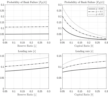
Figure 1 shows the effects of changes in capital and reserve requirements on the
probability of bank failure (FB(ˆx)) (upper subplots) and on the lending rate (r)
(lower subplots). The effects are displayed for three different values of the
(uncondi-tional) probability of default (p). As can be seen, increases in capital requirements
induce a decline in the probability of bank failure and an increase in the lending
rate. This result is in line with Repullo and Suarez (2004). Different values of
the probability of default (p) do not change the shape of the curves, though their
positions.
The results are different in case of reserve requirements. An increase in reserve
requirements of around ten percentage points triggers an increase in the lending rate
of around two percentage points. This compares to an increase in the lending rate
of similar size in case of a ten percentage points increase in capital requirements.
Hence the overall effects of reserve and capital requirements on the interest rate
spread are similar. The opposite though holds for the effects on the probability of
bank failure. In this case the differences are significant. Higher reserve requirements
induce negligibly small changes in the probability of bank failure – visually these
changes cannot be recognised. In the case of capital requirements, the effects on the
probability of bank failure are sizeable: a rise in capital requirements of up to fifteen
percentage points triggers a decline in the probability of bank failure of around ten
percentage points – the effects are weaker the smaller the probability of default (p).
Figure 1. Comparative statics
0.05 0.1 0.15 0.2 0.25 0.3
Reserve Ratio [ς]
0 0.05 0.1 0.15 0.2 0.25
0.3 Probability of Bank Failure [
FB(ˆx)]
0.05 0.1 0.15 0.2 0.25 0.3
Reserve Ratio [ς]
0 0.05 0.1 0.15
Lending rate [r]
0.05 0.1 0.15 0.2 0.25 0.3
Capital Ratio [k]
0 0.05 0.1 0.15 0.2 0.25
0.3 Probability of Bank Failure [
FB(ˆx)]
¯ p=0.05 ¯ p= 0.1 ¯ p=0.15
0.05 0.1 0.15 0.2 0.25 0.3
Capital Ratio [k]
0 0.05 0.1 0.15
Lending rate [r]
The negative effects of higher reserve requirements on the probability of bank
failure depend on the extent to which higher interest revenues from non-defaulting
loans compensate the losses from defaulting loans. This gives rise to assessing the
effects of reserve requirements on the probability of bank failure with respect to
the degree of loan-default correlation – this is captured by the parameter ϱ. If
ϱ → 1 then loan default rates are perfectly correlated as in the set-up of Section
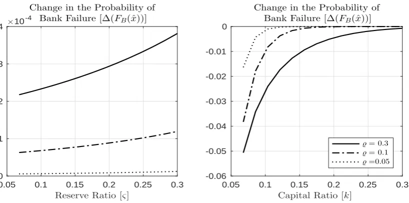
2.1. Figure 2 shows the effects of higher reserve and capital requirements on the
change in the probability of bank failure for different values of ϱ. As can be seen,
with a higher loan default correlation, rising reserve requirements lead to a larger
increase in the probability of bank failure. This shows that the contribution of
Figure 2. Comparative statics
0.05 0.1 0.15 0.2 0.25 0.3
Reserve Ratio [ς]
0 1 2 3 4×10
-4
Change in the Probability of Bank Failure [∆(FB(ˆx))]
0.05 0.1 0.15 0.2 0.25 0.3
Capital Ratio [k]
-0.06 -0.05 -0.04 -0.03 -0.02 -0.01 0
Change in the Probability of Bank Failure [∆(FB(ˆx))]
̺= 0.3 ̺= 0.1 ̺=0.05
default correlation increases. Hence the presence of imperfectly correlated
loan-default attenuates the negative effects of higher reserve requirements on financial
stability as the higher interest revenues from non-defaulting loans provide a buffer
for the losses from defaulting loans.
3. Optimal contracting problem
In the previous section, banks decide upon the structure of their assets by solving
a portfolio problem which trades off expected returns and the risk of failure. This
setup ignores the existence of a loan market. Moreover, in this environment banks
can control the level of riskdirectly. Within the approach of theoptimal contracting
problem, it is now entrepreneurs who are subject to a moral hazard problem. We
use a static model of Cournot competition in a market for entrepreneurial loans in
which the probability of default of loans is privately chosen by the entrepreneurs.
3.1. Reserves, capital and entrepreneurial risk-taking. The setup here
fol-lows the model of Boyd and De Nicol´o (2005); Mart´ınez-Miera and Repullo (2010);
Hakenes and Schnabel (2011) who consider an economy with two types of risk
neu-tral agents: entrepreneurs and banks. We assume that the return of projects of
different entrepreneurs is perfectly correlated. This implies that the probability of
Entrepreneurs. There is a continuum of entrepreneurs who have no own resources,
but have access to risky projects that require a unit investment and yield a stochastic
return
(26) R˜(pi) =
1 +α(pi), with probability 1−pi
0, with probability pi
where the probability of failure pi ∈ [0,1] is chosen privately by the entrepreneur.
As in Section 2.1 we assume that the success return of the project α(pi) > 0 is
concave withα′(0)> α(0) to get interior solutions.
To fund their projects entrepreneurs borrow from banks. Banks in turn cannot
ob-serve entrepreneurs’ risk-shifting choice pi, but take into account the best response
of entrepreneurs to their choice of the lending rate r. More specifically, the
en-trepreneurs’ choice ofpi at the beginning of the contract is unobservable for banks.
Afterwards, banks observe only whether the project has been successful. In this
environment, banks have no direct control over the riskiness of borrowers’ projects.
For any given loan rate r entrepreneur i will choose pi in order to maximize the
expected payoff from undertaking the project, which is the success return net of the
interest payment, α(pi)−r, multiplied by the probability of success, 1−pi, which
impliesp(r) = arg maxpi(1−pi)(α(pi)−r). Hence for any given loan rate r, all
en-trepreneurs will choose the samepi =p(r)∀i, which allows to omit the isubscript.
By our previous assumptions, the entrepreneurs’ objective function (1−p)(α(p)−r)
is concave, so that p(r) is obtained by solving the first-order condition
(27) r=α(p)−(1−p)α′(p)
For 0≤r < α(1) the solution will be interior. The cornerp= 0 cannot be a solution
ifα′(0)−α(0) +r >0, which holds by the assumption α′(0)> α(0), and the corner
p = 1 cannot be a solution if −α(1) +r < 0, that is for r < α(1). Differentiating
the first-order condition (27) we get
(28) p′(r) = −1
(1−p)α′′(p)−2α′(p) >0
Following Mart´ınez-Miera and Repullo (2010), we assume that each entrepreneur
is characterized by a continuous distribution of reservation utilities. Let Γ(u) denote
the measure of entrepreneurs that have a reservation utility less than or equal tou
and u(r) = maxp(1−p)(α(p)−r) determines the maximum expected payoff that
entrepreneurs can obtain when the loan rate isr. By the envelope theorem we have
u′(r) =−(1−p(r))<0 andu′′(r) = p′(r)>0. Entrepreneurs undertake the project
at the lending rate r if the reservation utility u is smaller than or equal to u(r).
Hence the measure of entrepreneurs that want to borrow from the banks at the
lending rate r is given by Γ(u(r)). Since each one requires a unit loan, the loan
demand function is
(29) L(r) = Γ(u(r))
Clearly for 0 ≤ r < α(1) we have L(r) > 0 with L′(r) = Γ′(u(r))u′(r) < 0 and
L′′(r) = Γ′(u(r))(u′(r))2 + Γ′(u(r))u′′(r) > 0. Let r(L) denote the corresponding
inverse loan demand function, which satisfies r′(L)<0 and r′′(L)>0.
Banks. The exposition of the banking sector closely follows Section 2.1. There is
a continuum of banks normalized to unity. Each bank i extends loans Li that are
financed by deposits Di and equity Ei. Additionally, banks have to hold reserves
Ri. As before, we assume that deposits are insured by a government-funded
de-posit scheme and, to simplify the presentation, we abstract from competition in
the deposit market by assuming that banks face a perfectly elastic supply of
de-posits at a rate equal to rD. Aggregate deposits in the banking sector are equal
to D = ∫1
0 Didi, the same applies for aggregate loans L =
∫1
0 Lidi and aggregate
reserves R = ∫1
0 Ridi. We assume that banks compete for loans `a la Cournot, so the strategic variable of a bank is the supply of loansLi. Finally, we assume that a
regulator imposes a minimum reserve and capital requirementς andk, i.e. Ei ≥kLi
and Ri ≥ςDi.
3.2. Equilibrium. We solve the model by backward induction and consider
sym-metric equilibria only. In a Nash equilibrium, each bank chooses loans and the
amount of reserves and capital to maximize profits, given similar choices of the
the projects. In this setup, banks lend to entrepreneurs whose returns are perfectly
correlated. This assumption is equivalent to the one taken in Section 2.1 on a bank
portfolio composed of perfectly correlated risks. This implies that the probability
of default of loans p(r(L)) coincides with the probability of bank failure FB.
Banks maximize the present discounted value of their net worth π(L) net of
bankers’ initial infusion of capital
(30) V = max
{L,k,ς} [
−k+ 1
1 +δπ(L) ]
L
and the net worth per unit of loanπ(L) is given by
(31) π(L) = [1−p(r(L))]
(
r(L) +k−rD1−k
1−ς )
Banks choose the profit maximizing volumes of loansL and decide upon how much
capitalk and reserves ς to hold per unit of loan and deposit. Importantly, though,
is the fact that the aggregate supply of loans L determines the lending rate r(L),
which in turn determines the probability of failure chosen by the entrepreneurs as
implied by equation (27). Taken together, this motivates p(r(L)) being implicitly
defined by equations (27) and (29).
The first order conditions with respect to reserve holdingsς and capital holdingsk
are equivalent to equations (6) and (7). As before, banks do not hold equity capital
and reserves in excess of what is required by prudential regulation. The first order
condition with respect to the amount of loans is given by
(32) r(L)−rD1−k
1−ς =
1 +δ−g(L)
g(L) k+G(L)
where g(L) ≡ 1− p(r(L))− Lp′(r(L))r′(L) > 0 since5 r′(L) < 0 and G(L) ≡ −[1−p(r(L))]r′(L)L
g(L)) > 0 with G
′(L) > 0 as shown implicitly in Boyd and De Nicol´o
(2005). Equation (32) defines the equilibrium lending rater(L) as a function of the
cost of equity(1+δg−(Lg)(L)k), the cost of deposits( rD1−k
1−ς )
and some “monopoly rents”
captured by G(L). Equation (32) is to be compared with equation (8) from the
setup based on portfolio optimization. In contrast to equation (8), equation (32)
5Note that g(L) can be expressed in terms of risk and loan elasticities: g(L) = 1 +
p(r(L))(
contains the cost of capital δ. This is because in the model outlined in Section 2.1,
the volume of loans is irrelevant for banks’ profits; the only decisive factor is the
composition of loans in terms of the degree of risk they contain. Within the setup
of the optimal contracting problem, changes in the loan volume imply changes in
revenues due to the downward sloping inverse demand function r(L) for loans.
3.3. Implications of reserve and capital regulation. We now analyse how
re-serve and capital regulation affect the probability of bank failure. For this we focus
on the effects of prudential regulation on the degree of riskiness p(r(L)) of a single
loan and banks’ probability of default FB. By assumption, the return of projects
of different entrepreneurs is perfectly correlated. This implies that the probability
of entrepreneurs’ default on their loans p(r(L)) coincides with the probability of
bank failureFB =p(r(L)). We will see that (i) reserve requirements have a unique
effect on the probability of bank failure and (ii) the sign of the effects of capital
requirements on the probability of bank failure depends on reserve requirements.
We proceed stepwise to assess the effects of changes in reserve and capital
re-quirements. For this, we first determine their effects on loan supply. This result
will then be used to evaluate the effect on the lending rate and the degree of
risk-taking by entrepreneurs. From this we can then determine the probability of bank
failure. We define γ(L) ≡ G′(L)−r′(L)−kg′(L)(1+δ)
g(L)2 which satisfies γ(L) > 0 if
G′(L)−r′(L) > kg′(L)(1+δ)
g(L)2 which we assume applies. Considering the total
differ-ential of equation (32) we find the following for the partial effects of reserve and
capital requirements on loan supply
dL
dς = −
rD γ(L)
1−k
(1−ς)2 <0 (33)
dL
dk =
1
γ(L)
(
1−ς+rD
1−ς −
1 +δ g(L)
)
<0 if 1−ς+rD 1−ς <
1 +δ g(L) (34)
Sincer(L) is the inverse demand function for loans, we have thatdr(L)/dς >0 and
dr(L)/dk >0 if 1−1ς−+ςrD < 1+δ
g(L). Finally, taking the total differential of FB =p(r(L))
probability of bank failure
dFB
dς = p
′(r(L))r′(L)dL dς >0
(35)
dFB
dk = p
′(r(L))r′(L)dL dk >0 if
1−ς+rD
1−ς <
1 +δ g(L) (36)
Equation (35) highlights that the overall effect of changes in reserve requirements
on the probability of bank failure depends on three components: (i) the extent to
which changes in reserves trigger changes in loan supply (dL/dς), (ii) the extent to
which changes in the loan supply affect the lending rate by means of the demand
function for loans (r′(L)), and (iii) the extent to which changes in the lending rate
affect risk-taking by entrepreneurs (p′(r(L))).
For a more intuitive explanation, consider an increase in the reserve requirement
ς. This implies that now a larger part of the deposit volume cannot be used for
loan supply. Hence higher reserve requirements render deposits more expensive
inducing banks to a reduction (substitution effect). The reduction in deposits could
in principle be counterbalanced with equity capital, however, this is not the case since
capital is only held to the amount necessary as required by prudential regulation
which is due to equation (7). Hence the decline in deposits brings about a decrease
in the aggregate loan volume L which translates into an increase in the lending
rate r(L). This in turn promotes higher risk-taking by entrepreneurs. Hence, a
tighter reserve regulation increases the risk of individual loans. Put differently,
reserve requirements do not contribute to financial stability as higher reserves fail
in ameliorating entrepreneurs’ moral hazard problem. Importantly, the size of the
adverse effects of higher reserve requirements crucially depends on entrepreneurs’
risk-taking sensitivity.
In this environment, capital requirements determine the size of the effects of
changes in reserve requirements on the probability of bank failure, though, they
leave the sign of the effects unchanged. The opposite, in turn, applies for capital
regulation as highlighted by equation (36). Whenς →0, then 1−ς+rD
1−ς is comparably
small rendering more likely 1−1ς−+ςrD < g1+(Lδ). In this case, stricter capital requirements
increase a bank’s probability of failure. This replicates Proposition 3 in Hakenes
and Schnabel (2011): an increase in the capital requirement raises capital costs,
decrease in the aggregate loan volume L translates into an increase in the lending
rate and into higher risk-taking by entrepreneurs. Hence, a tighter capital
regula-tion increases the risk of individual loans because it exacerbates the entrepreneurs’
moral hazard problem. However, equation (36) highlights that this effect strongly
depends on the reserve regulation. When ς → 1, then 1−ς+rD
1−ς is comparably large
with the likely consequence that 1−ς+rD
1−ς >
1+δ
g(L). In this case
dp(r(L))
dk < 0, implying
that when reserve requirements are already high, increases in capital requirements
have the potential to reduce banks’ probability of failure.
This example highlights that, first of all, higher reserve requirements increase the
probability of bank failure since they promote entrepreneurial risk taking. Secondly,
the regulatory stance on reserve requirements determines not only the effectiveness
of capital requirements but, even more importantly, the sign.
3.4. Numerical results. In the following we use numerical methods to illustrate
the effects of reserve and capital requirements in an environment of optimal
contract-ing. We follow Mart´ınez-Miera and Repullo (2010) and utilize a simple
parametriza-tion based on the assumpparametriza-tion of linearity for the inverse demand for loansr(L) and
the entrepreneurial risk-shifting function p(r). This allows us to quantitatively
as-sess the effects of changes in reserve and capital requirements on the probability of
bank failureFB =p(r(L)).
We postulate an entrepreneurial risk-shifting function p(r) and an inverse loan
demand function r(L) of the forms
(37) p(r) = a+b·r and r(L) =c−d·L
witha >0,b >0,c > 0 and d >0. In this setup, the parameter acharacterizes the
probability of default of a project chosen by entrepreneurs when the lending rate r
is equal to zero (that is, the minimum default probability of a project) and the ratio
c/d gives the maximum volume of loans which occurs at a lending rate r equal to
zero.6 For the parametrization we take a= 0.01, b= 0.5, c= 1, and d = 0.01. This
6As highlighted in Mart´ınez-Miera and Repullo (2010), the linear functional form for p(r) can
Figure 3. Comparative statics
0.05 0.1 0.15 0.2 0.25 0.3
Reserve Ratio [ς]
0 0.02 0.04 0.06 0.08
0.1 Probability of Bank Failure [
FB]
0.05 0.1 0.15 0.2 0.25 0.3
Reserve Ratio [ς]
0.075 0.08 0.085 0.09 0.095 0.1
0.105 Lending rate [
r]
b= 0.8
b= 0.5
b=0.05
0.05 0.1 0.15 0.2 0.25 0.3
Capital Ratio [k]
0 0.02 0.04 0.06 0.08
0.1 Probability of Bank Failure [
FB]
0.05 0.1 0.15 0.2 0.25 0.3
Capital Ratio [k]
0.075 0.08 0.085 0.09 0.095 0.1
0.105 Lending rate [
r]
means that the demand for loans goes from 100 to 0 as loan rates range from 0%
to 100%, and that the probability of default p that corresponds to a loan rate of
2% is equal to 2%. The default value chosen for reserve and capital requirements is
ς =k = 0.1.
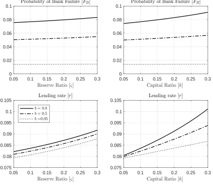
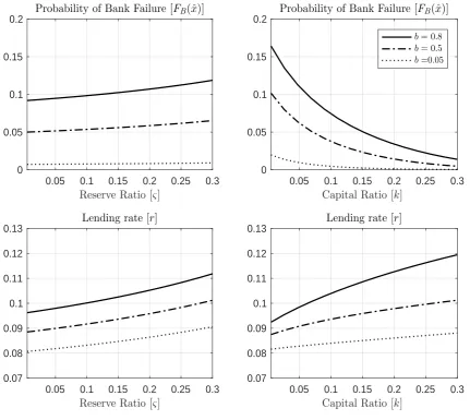
Figure 3 shows the effects of changes in reserve and capital requirements on the
lending rate (r) and the probability of bank failure (FB) resulting from the model
which is characterized by equation (32) and the equations in (37). The simulations
distinguish between different degrees of entrepreneurs’ risk-taking sensitivity
cap-tured by the parameter b – higher values of b imply a higher sensitivity towards
risk. The subplots in the left panel of the figure highlight that higher reserve
Figure 4. Comparative statics
0.05 0.1 0.15 0.2 0.25 0.3
Reserve Ratio [ς]
0.03 0.04 0.05 0.06 0.07
0.08 Probability of Bank Failure [
FB]
k=0.05
k=0.95
0.05 0.1 0.15 0.2 0.25 0.3
Reserve Ratio [ς]
0.06 0.08 0.1 0.12 0.14
0.16 Lending rate [
r]
0.05 0.1 0.15 0.2 0.25 0.3
Capital Ratio [k]
0 0.05 0.1 0.15 0.2
0.25 Probability of Bank Failure [
FB]
ς=0.05 ς=0.95
0.05 0.1 0.15 0.2 0.25 0.3
Capital Ratio [k]
0 0.1 0.2 0.3 0.4
0.5 Lending rate [
r]
rate alike. This applies for any value of the risk-shifting parameter b. The higher
entrepreneurs’ risk sensitivity, the larger is the increase in the probability of bank
failure induced by increases in reserve requirements. The same applies to capital
requirements. If, in turn, b = 0, then changes in reserve and capital requirements
would leave the probability of bank failure unaffected as highlighted by equations
(35) and (36). Hence the effects of both reserve and capital requirements on the
probability of bank failure crucially depend on entrepreneurs’ risk-taking preference.
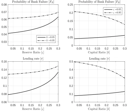
Figure 4 shows the effects of higher reserve and capital requirements on the
proba-bility of bank failure and the lending rate for concurrent values of capital and reserve
requirements of a certain amount. The effects of reserve requirements are shown for
be seen, different values for capital requirements hardly change the shape of the
curve, though its position. Most importantly, capital requirements have no ability
in changing the sign of the effects of reserve requirements on the probability of bank
failure. The opposite applies to capital requirements. The two subplots in the right
panel of Figure 4 show that when reserve requirements are high, increases in capital
requirements contribute to ameliorate entrepreneurs’ moral hazard problem in the
choice of risk and hence to a decrease in the probability of bank failure. The
oppo-site applies at low values for reserve requirements. This example illustrates how the
interaction between reserve and capital requirements matters for the effectiveness
and even the sign of the effects of these regulatory tools.
4. The role of entrepreneurial risk-shifting and imperfectly
correlated loan default
As a final attempt to assess the role of reserve regulation on bank risk-taking, we
now consider its effects within a model that considers jointly the portfolio problem
and the optimal contracting problem. Specifically, we merge the models considered
in Sections 2.2 and 3 with minor changes. Hence the basic setup is identical to that
of Mart´ınez-Miera and Repullo (2010) except for the introduction of reserve and
capital regulation as motivated in Section 2.1.
Entrepreneurs. As in Section 3, we consider a continuum of entrepreneurs who have
no own resources, but have access to risky projects that require a unit investment
and yields a stochastic return
(38) R˜(pi) =
1 +α(pi), with probability 1−pi
1−λ, with probability pi
where 0< λ <1 is an individual project’s LGD and to simplify the presentation we
assume that it does not depend on pi. In contrast to Section 3.1, we now assume
that project failures and consequently loan defaults are imperfectly correlated. For
this we use the single risk factor model of Vasicek (2002), which introduces the
Banks. The structure of the banking sector follows the setup of Section 2.2 and
Section 3.1 with minor modifications to account for the different risk environment.
Assuming that banks compete for loans `a la Cournot, so as in Section 3, the strategic
variable of a bank i is its supply of loans Li. Bank i’s net worth π(Li, L) per unit
of loan Li is again given by equation (14), though, it now depends on aggregate
loansL, which in turn results from the dependence of lending rates on the aggregate
volume of loans (r = r(L)). The bank fails when π(Li, L) < 0, that is, when the
default rate x is greater than the bankruptcy/default rate ˆx(L) which is given by
equation (18) and depends on loans Lsince the lending rate r(L) is now a function
of loans.7
As before, bank i’s objective is to maximize the expected discounted value of
max(π(Li, L),0), net of bankers’ initial infusion of capital, which now reads
(39) Vi(Li) =Li·
[
−k+ 1 1 +δ
∫ xˆ(L)
0
π(L)dF(x;p(r(L)))
]
where the distribution functionF(x;p(r(L))) of the default ratexis written so as to
account for the endogenous probability of default of the loans. Thus, when banki
chooses its supply of loansLi, it takes into account (i) the direct effect of changes in
loan supply on the lending rater(L), and (ii) the indirect effect on the probability of
default of the loansp(r(L)) and hence on the probability distribution of the default
rate x.
Bankimaximizes the expected discounted valueVi with respect to the amount of
capitalk and reservesς; optimization yields the same first order conditions as given
by equations (16) and (17). Hence, bank i will always hold the minimum amount
of reserves and capital as required by the regulation.
4.1. Equilibrium. In what follows, we identify the Cournot symmetric equilibrium
of the model of competition in the loan market with imperfectly correlated loan
default, and analyse the effect of changes in reserve and capital requirements on
the equilibrium lending rate r(L) and the equilibrium probability of bank failure
FB(L) = 1−F(ˆx(L);p(r(L))).
7Equivalently to Section 2.1, the bankruptcy/default rate ˆx(L) could also be derived formally by
The assumption of symmetry simplifies the model and implies Li = L. Using
equation (18) for the bankruptcy/default rate ˆx(L) and applying integration by
parts allows to re-write equation (39) in the following way
(40) V(L) =Lπ(L)
with π(L) being the net worth per unit of loanL given by
(41) π(L) =−k+λ+r(L)
1 +δ
∫ xˆ(L)
0
F(x;p(r(L)))dx
The first order condition with respect to loans L yields the following first-order
differential equation
(42) π(L) =−Lπ′(L)
whereπ′(L) is given by
π′(L) = r ′(L)
1 +δ [
(1−xˆ(L))F(ˆx(L);p(r(L))) + (43)
∫ xˆ(L)
0
(
F(x;p(r(L))) + (λ+r(L))∂F(x;p(r(L)))
∂p(r(L)) p
′(r(L)) )
dx ]
and we used ˆx′(L) = 1−xˆ(L)
λ+r(L)r
′(L)<0 as implied by equation (18). The first term in
square brackets in equation (43) is positive. The sign of the term within the integral
is ambiguous because F(x;p(r(L))) > 0, whereas ∂F∂p(x(;pr((rL())L))) < 0 (the effect on
the probability distribution of the bankruptcy/default rate) andp′(r(L))>0
(risk-shifting effect). In line with Mart´ınez-Miera and Repullo (2010), we assume that the
parametrization and functional forms are such thatπ′(L)<0 andπ′′(L)<0, so that
there is a unique symmetric equilibrium. The complication arises from the effect of
the bankruptcy/default rate on the probability distribution (∂F∂p(x;(pr((rL())L))) <0). To
see this, assume that loan defaults are perfectly correlated (ϱ → 1). This implies
thatF(x;p(r(L))) = 1−p(r(L)) for 0≤x≤1 and hence by using equation (18) and
(41) we obtainπ(L) = [1−p(r(L))](
r(L) +k−rD1−k
1−ς )
which is the net worth per
unit of loan as given in equation (4) of the model based on theportfolio problemwith
perfectly correlated loan default and it also corresponds to the net worth defined in
equation (31) of the model based on theoptimal contracting problem with perfectly