A Trainable Spaced Repetition Model for Language Learning
Burr Settles∗ Duolingo Pittsburgh, PA USA [email protected]
Brendan Meeder†
Uber Advanced Technologies Center Pittsburgh, PA USA
Abstract
We present half-life regression (HLR), a novel model for spaced repetition practice with applications to second language ac-quisition. HLR combines psycholinguis-tic theory with modern machine learning techniques, indirectly estimating the “half-life” of a word or concept in a student’s long-term memory. We use data from Duolingo — a popular online language learning application — to fit HLR models, reducing error by 45%+ compared to sev-eral baselines at predicting student recall rates. HLR model weights also shed light on which linguistic concepts are system-atically challenging for second language learners. Finally, HLR was able to im-prove Duolingo daily student engagement by 12% in an operational user study. 1 Introduction
The spacing effect is the observation that people tend to remember things more effectively if they usespaced repetition practice(short study periods spread out over time) as opposed tomassed prac-tice(i.e., “cramming”). The phenomenon was first documented by Ebbinghaus (1885), using himself as a subject in several experiments to memorize verbal utterances. In one study, after a day of cramming he could accurately recite 12-syllable sequences (of gibberish, apparently). However, he could achieve comparable results with half as many practices spread out over three days.
Thelag effect(Melton, 1970) is the related ob-servation that people learn even better if the spac-ing between practices gradually increases. For ex-ample, a learning schedule might begin with
re-∗Corresponding author.
†Research conducted at Duolingo.
view sessions a few seconds apart, then minutes, then hours, days, months, and so on, with each successive review stretching out over a longer and longer time interval.
The effects of spacing and lag are well-established in second language acquisition re-search (Atkinson, 1972; Bloom and Shuell, 1981; Cepeda et al., 2006; Pavlik Jr and Anderson, 2008), and benefits have also been shown for gym-nastics, baseball pitching, video games, and many other skills. See Ruth (1928), Dempster (1989), and Donovan and Radosevich (1999) for thorough meta-analyses spanning several decades.
Most practical algorithms for spaced repetition are simple functions with a few hand-picked pa-rameters. This is reasonable, since they were largely developed during the 1960s–80s, when people would have had to manage practice sched-ules without the aid of computers. However, the recent popularity of large-scale online learning software makes it possible to collect vast amounts of parallel student data, which can be used to em-pirically train richer statistical models.
In this work, we propose half-life regression (HLR)as a trainable spaced repetition algorithm, marrying psycholinguistically-inspired models of memory with modern machine learning tech-niques. We apply this model to real student ing data from Duolingo, a popular language learn-ing app, and use it to improve its large-scale, op-erational, personalized learning system.
2 Duolingo
Duolingo is a free, award-winning, online lan-guage learning platform. Since launching in 2012, more than 150 million students from all over the world have enrolled in a Duolingo course, either via the website1or mobile apps for Android, iOS,
1https://www.duolingo.com
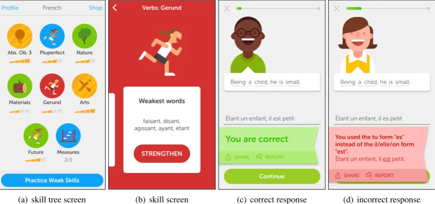
(a) skill tree screen (b) skill screen (c) correct response (d) incorrect response Figure 1: Duolingo screenshots for an English-speaking student learning French (iPhone app, 2016). (a) A course skill tree: golden skills have four bars and are “at full strength,” while other skills have fewer bars and are due for practice. (b) A skill screen detail (for theGerundskill), showing which words are predicted to need practice. (c,d) Grading and explanations for a translation exercise.
´etant un enfant il est petit
ˆetre.V.GER un.DET.INDF.M.SG enfant.N.SG il.PN.M.P3.SG ˆetre.V.PRES.P3.SG petit.ADJ.M.SG
Figure 2: The French sentence from Figure 1(c,d) and its lexeme tags. Tags encode the root lexeme, part of speech, and morphological components (tense, gender, person, etc.) for each word in the exercise.
and Windows devices. For comparison, that is more than the total number of students in U.S. el-ementary and secondary schools combined. At least 80 language courses are currently available or under development2for the Duolingo platform. The most popular courses are for learning English, Spanish, French, and German, although there are also courses for minority languages (Irish Gaelic), and even constructed languages (Esperanto).
More than half of Duolingo students live in developing countries, where Internet access has more than tripled in the past three years (ITU and UNESCO, 2015). The majority of these students are using Duolingo to learn English, which can significantly improve their job prospects and qual-ity of life (Pinon and Haydon, 2010).
2.1 System Overview
Duolingo uses a playfully illustrated, gamified de-sign that combines point-reward incentives with implicit instruction (DeKeyser, 2008), mastery learning (Block et al., 1971), explanations (Fahy,
2https://incubator.duolingo.com
2004), and other best practices. Early research suggests that 34 hours of Duolingo is equivalent to a full semester of university-level Spanish in-struction (Vesselinov and Grego, 2012).
Each language course also contains a corpus
(large database of available exercises) and a lex-eme tagger(statistical NLP pipeline for automat-ically tagging and indexing the corpus; see the Appendix for details and a lexeme tag reference). Figure 1(c,d) shows an example translation exer-cise that might appear in theGerundskill, and Fig-ure 2 shows the lexeme tagger output for this sen-tence. Since this exercise is indexed with a gerund lexeme tag (ˆetre.V.GERin this case), it is available for lessons or practices in this skill.
The lexeme tagger also helps to provide correc-tive feedback. Educational researchers maintain that incorrect answers should be accompanied by
explanations, not simply a “wrong” mark (Fahy, 2004). In Figure 1(d), the student incorrectly used the 2nd-person verb form es(ˆetre.V.PRES.P2.SG) instead of the 3rd-personest(ˆetre.V.PRES.P3.SG). If Duolingo is able to parse the student response and detect a known grammatical mistake such as this, it provides an explanation3in plain language. Each lesson continues until the student masters all of thetarget wordsbeing taught in the session, as estimated by a mixture model of short-term learn-ing curves (Streeter, 2015).
2.2 Spaced Repetition and Practice
Once a lesson is completed, all the target words being taught in the lesson are added to thestudent model. This model captures what the student has learned, and estimates how well she can recall this knowledge at any given time. Spaced repetition is a key component of the student model: over time, the strength of a skill will decay in the student’s long-term memory, and this model helps the stu-dent manage her practice schedule.
Duolingo usesstrength metersto visualize the student model, as seen beneath each of the com-pleted skill icons in Figure 1(a). These meters represent the average probability that the student can, at any moment, correctly recall a random tar-get word from the lessons in this skill (more on this probability estimate in§3.3). At four bars, the skill is “golden” and considered fresh in the stu-dent’s memory. At fewer bars, the skill has grown stale and may need practice. A student can tap the skill icon to access practice sessions and target her weakest words. For example, Figure 1(b) shows
3If Duolingo cannot parse the precise nature of the
mis-take — e.g., because of a gross typographical error — it pro-vides a “diff” of the student’s response with the closest ac-ceptable answer in the corpus (using Levenshtein distance).
some weak words from theGerundskill. Practice sessions are identical to lessons, except that the exercises are taken from those indexed with words (lexeme tags) due for practice according to student model. As time passes, strength meters continu-ously update and decay until the student practices. 3 Spaced Repetition Models
In this section, we describe several spaced repeti-tion algorithms that might be incorporated into our student model. We begin with two common, estab-lished methods in language learning technology, and then present our half-life regression model which is a generalization of them.
3.1 The Pimsleur Method
Pimsleur (1967) was perhaps the first to make mainstream practical use of the spacing and lag ef-fects, with his audio-based language learning pro-gram (now a franchise by Simon & Schuster). He referred to his method as graduated-interval re-call, whereby new vocabulary is introduced and then tested at exponentially increasing intervals, interspersed with the introduction or review of other vocabulary. However, this approach is lim-ited since the schedule is pre-recorded and can-not adapt to the learner’s actual ability. Consider an English-speaking French student who easily learns a cognate like pantalon (pants), but strug-gles to remembermanteau(coat). With the Pim-sleur method, she is forced to practice both words at the same fixed, increasing schedule.
3.2 The Leitner System
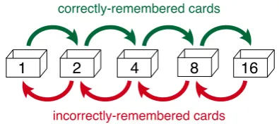
Leitner (1972) proposed a different spaced repeti-tion algorithm intended for use with flashcards. It is more adaptive than Pimsleur’s, since the spac-ing intervals can increase or decrease dependspac-ing on student performance. Figure 3 illustrates a pop-ular variant of this method.
1 2 4 8 16
correctly-remembered cards
[image:3.595.317.515.611.699.2]incorrectly-remembered cards
Figure 3: The Leitner System for flashcards.
4-day, and so on. All cards start out in the 1-day box, and if the student can remember an item after one day, it gets “promoted” to the 2-day box. Two days later, if she remembers it again, it gets pro-moted to the 4-day box, etc. Conversely, if she is incorrect, the card gets “demoted” to a shorter in-terval box. Using this approach, the hypothetical French student from§3.1 would quickly promote
pantalonto a less frequent practice schedule, but continue reviewing manteau often until she can regularly remember it.
Several electronic flashcard programs use the Leitner system to schedule practice, by organiz-ing items into “virtual” boxes. In fact, when it first launched, Duolingo used a variant similar to Fig-ure 3 to manage skill meter decay and practice. The present research was motivated by the need for a more accurate model, in response to student complaints that the Leitner-based skill meters did not adequately reflect what they had learned.
3.3 Half-Life Regression: A New Approach
We now describe half-life regression (HLR), start-ing from psychological theory and combinstart-ing it with modern machine learning techniques.
Central to the theory of memory is the Ebbing-haus model, also known as the forgetting curve
(Ebbinghaus, 1885). This posits that memory de-cays exponentially over time:
p= 2−∆/h. (1)
In this equation,pdenotes the probability of cor-rectly recalling an item (e.g., a word), which is a function of ∆, the lag timesince the item was last practiced, and h, thehalf-life or measure of strength in the learner’s long-term memory.
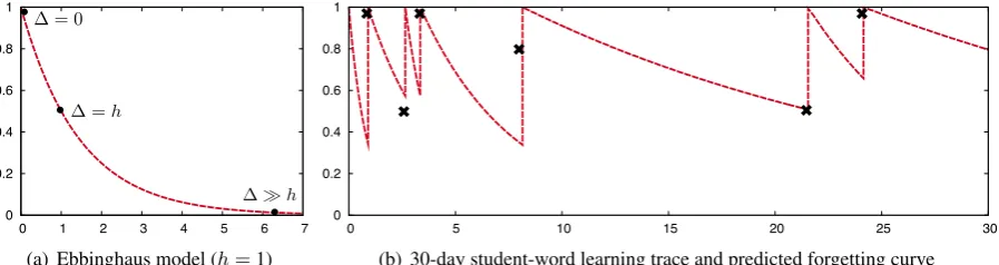
Figure 4(a) shows a forgetting curve (1) with half-lifeh=1. Consider the following cases:
1. ∆ =0. The word was just recently practiced, sop= 20 =1.0, conforming to the idea that
it is fresh in memory and should be recalled correctly regardless of half-life.
2. ∆ =h. The lag time is equal to the half-life, sop = 2−1 =0.5, and the student is on the
verge of being unable to remember.
3. ∆h. The word has not been practiced for a long time relative to its half-life, so it has probably been forgotten, e.g.,p≈0.
Let xdenote a feature vector that summarizes a student’s previous exposure to a particular word, and let the parameter vectorΘcontain weights that correspond to each feature variable in x. Under the assumption that half-life should increase expo-nentially with each repeated exposure (a common practice in spacing and lag effect research), we let
ˆ
hΘdenote the estimated half-life, given by: ˆ
hΘ= 2Θ·x. (2)
In fact, the Pimsleur and Leitner algorithms can be interpreted as special cases of (2) using a few fixed, hand-picked weights. See the Appendix for the derivation ofΘfor these two methods.
For our purposes, however, we want to fitΘ em-pirically to learning trace data, and accommodate an arbitrarily large set of interesting features (we discuss these features more in§3.4). Suppose we have a data setD = {hp,∆,xii}Di=1 made up of
student-word practice sessions. Each data instance consists of the observed recall ratep4, lag time∆ since the word was last seen, and a feature vector
xdesigned to help personalize the learning expe-rience. Our goal is to find the best model weights
Θ∗to minimize some loss function`:
Θ∗ = arg min Θ
D X
i=1
`(hp,∆,xii; Θ). (3)
To illustrate, Figure 4(b) shows a student-word learning trace over the course of a month. Each 6indicates a data instance: the vertical position is the observed recall ratepfor each practice session, and the horizontal distance between points is the lag time∆between sessions. Combining (1) and (2), the model prediction pˆΘ = 2−∆/ˆhΘ is
plot-ted as a dashed line over time (which resets to 1.0 after each exposure, since∆ =0). The training loss function (3) aims to fit the predicted forget-ting curves to observed data points for millions of student-word learning traces like this one.
We chose theL2-regularized squared loss
func-tion, which in its basic form is given by: `(6; Θ) = (p−pˆΘ)2+λkΘk22 ,
where6 =hp,∆,xiis shorthand for the training data instance, andλis a parameter to control the regularization term and help prevent overfitting.
4In our setting, each data instance represents a full lession
0 0.2 0.4 0.6 0.8 1
0 1 2 3 4 5 6 7
!
!
!
(a) Ebbinghaus model (h=1) 0 0.2 0.4 0.6 0.8 1
0 5 10 15 20 25 30 ✖
✖ ✖
✖
✖
✖
[image:5.595.77.526.62.181.2](b) 30-day student-word learning trace and predicted forgetting curve
Figure 4: Forgetting curves. (a) Predicted recall rate as a function of lag time∆and half-lifeh =1. (b) Example student-word learning trace over 30 days: 6 marks the observed recall rate p for each practice session, and half-life regression aims to fit model predictionspˆΘ(dashed lines) to these points.
In practice, we found it useful to optimize for the half-life h in addition to the observed recall ratep. Since we do not know the “true” half-life of a given word in the student’s memory — this is a hypothetical construct — we approximate it algebraically from (1) using p and ∆. We solve forh= log−∆
2(p) and use the final loss function:
`(6; Θ) = (p−pˆΘ)2+α(h−ˆhΘ)2+λkΘk22 ,
whereαis a parameter to control the relative im-portance of the half-life term in the overall train-ing objective function. Since`is smooth with re-spect toΘ, we can fit the weights to student-word learning traces using gradient descent. See the Ap-pendix for more details on our training and opti-mization procedures.
3.4 Feature Sets
In this work, we focused on features that were eas-ily instrumented and available in the production Duolingo system, without adding latency to the student’s user experience. These features fall into two broad categories:
• Interaction features: a set of counters sum-marizing each student’s practice history with each word (lexeme tag). These include the total number of times a student has seen the wordxn, the number of times it was correctly
recalledx⊕, and the number of times incor-rectx . These are intended to help the model make more personalized predictions.
• Lexeme tag features: a large, sparse set of indicator variables, one for each lexeme tag in the system (about 20k in total). These are intended to capture the inherent difficulty of each particular word (lexeme tag).
recall rate lag (days) feature vectorx
p (⊕/n) ∆ xn x⊕ x xˆetre.V.GER
1.0 (3/3) 0.6 3 2 1 1
0.5 (2/4) 1.7 6 5 1 1
1.0 (3/3) 0.7 10 7 3 1
0.8 (4/5) 4.7 13 10 3 1
0.5 (1/2) 13.5 18 14 4 1
1.0 (3/3) 2.6 20 15 5 1
Table 1: Example training instances. Each row corresponds to a data point in Figure 4(b) above, which is for a student learning the French word
´etant(lexeme tagˆetre.V.GER).
To be more concrete, imagine that the trace in Figure 4(b) is for a student learning the French word´etant(lexeme tagˆetre.V.GER). Table 1 shows what hp,∆,xi would look like for each session in the student’s history with that word. The inter-action features increase monotonically5over time, andxˆetre.V.GER is the only lexeme feature to “fire”
for these instances (it has value 1, all other lexeme features have value 0). The model also includes a bias weight (intercept) not shown here.
4 Experiments
In this section, we compare variants of HLR with other spaced repetition algorithms in the context of Duolingo. First, we evaluate methods against his-torical log data, and analyze trained model weights for insight. We then describe two controlled user experiments where we deployed HLR as part of the student model in the production system.
5Note that in practice, we found that using the square root
of interaction feature counts (e.g.,√x⊕) yielded better
Model MAE↓ AUC↑ CORh↑
HLR 0.128* 0.538* 0.201* HLR -lex 0.128* 0.537* 0.160* HLR -h 0.350 0.528* -0.143* HLR -lex-h 0.350 0.528* -0.142* Leitner 0.235 0.542* -0.098* Pimsleur 0.445 0.510* -0.132*
LR 0.211 0.513* n/a
LR -lex 0.212 0.514* n/a
Constantp¯=0.859 0.175 n/a n/a
Table 2: Evaluation results using historical log data (see text). Arrows indicate whether lower (↓) or higher (↑) scores are better. The best method for each metric is shown in bold, and statistically significant effects (p <0.001) are marked with *.
4.1 Historical Log Data Evaluation
We collected two weeks of Duolingo log data, containing 12.9 million student-word lesson and practice session traces similar to Table 1 (for all students in all courses). We then compared three categories of spaced repetition algorithms:
• Half-life regression (HLR), our model from
§3.3. For ablation purposes, we consider four variants: with and without lexeme features (-lex), as well as with and without the half-life term in the loss function (-h).
• Leitner and Pimsleur, two established base-lines that are special cases of HLR, using fixed weights. See the Appendix for a deriva-tion of the model weights we used.
• Logistic regression (LR), a standard machine learning6baseline. We evaluate two variants: with and without lexeme features (-lex).
We used the first 1 million instances of the data to tune the parameters for our training algorithm. After trying a handful of values, we settled on λ =0.1,α =0.01, and learning rate η =0.001. We used these same training parameters for HLR and LR experiments (the Leitner and Pimsleur models are fixed and do not require training).
6For LR models, we include the lag timex
∆as an
addi-tional feature, since — unlike HLR — it isn’t explicitly ac-counted for in the model. We experimented with polynomial and exponential transformations of this feature, as well, but found the raw lag time to work best.
Table 2 shows the evaluation results on the full data set of 12.9 million instances, using the first 90% for training and remaining 10% for testing. We consider several different evaluation measures for a comprehensive comparison:
• Mean absolute error (MAE) measures how closely predictions resemble their observed outcomes: 1
D
PD
i=1|p−pˆΘ|i. Since the
strength meters in Duolingo’s interface are based on model predictions, we use MAE as a measure of prediction quality.
• Area under the ROC curve (AUC)— or the Wilcoxon rank-sum test — is a measure of ranking quality. Here, it represents the proba-bility that a model ranks a random correctly-recalled word as more likely than a random incorrectly-recalled word. Since our model is used to prioritize words for practice, we use AUC to help evaluate these rankings.
• Half-life correlation (CORh)is the Spearman
rank correlation between ˆhΘ and the
alge-braic estimate h described in§3.3. We use this as another measure of ranking quality. For all three metrics, HLR with lexeme tag fea-tures is the best (or second best) approach, fol-lowed closely by HLR -lex (no lexeme tags). In fact, these are the only two approaches with MAE lower than a baseline constant prediction of the av-eragerecall rate in the training data (Table 2, bot-tom row). These HLR variants are also the only methods with positive CORh, although this seems
reasonable since they are the only two to directly optimize for it. While lexeme tag features made limited impact, theh term in the HLR loss func-tion is clearly important: MAE more than doubles without it, and the -hvariants are generally worse than the other baselines on at least one metric.
As stated in§3.2, Leitner was the spaced repeti-tion algorithm used in Duolingo’s producrepeti-tion stu-dent model at the time of this study. The Leitner method did yield the highest AUC7values among the algorithms we tried. However, the top two HLR variants are not far behind, and they also re-duce MAE compared to Leitner by least 45%.
7AUC of 0.5 implies random guessing (Fawcett, 2006),
Lg. Word Lexeme Tag θk
EN camera camera.N.SG 0.77 EN ends end.V.PRES.P3.SG 0.38 EN circle circle.N.SG 0.08
EN rose rise.V.PST -0.09
EN performed perform.V.PP -0.48 EN writing write.V.PRESP -0.81
ES liberal liberal.ADJ.SG 0.83 ES como comer.V.PRES.P1.SG 0.40 ES encuentra encontrar.V.PRES.P3.SG 0.10 ES est´a estar.V.PRES.P3.SG -0.05 ES pensando pensar.V.GER -0.33 ES quedado quedar.V.PP.M.SG -0.73
FR visite visiter.V.PRES.P3.SG 0.94 FR suis ˆetre.V.PRES.P1.SG 0.47
FR trou trou.N.M.SG 0.05
FR dessous dessous.ADV -0.06
FR ceci ceci.PN.NT -0.45
FR fallait falloir.V.IMPERF.P3.SG -0.91
DE Baby Baby.N.NT.SG.ACC 0.87 DE sprechen sprechen.V.INF 0.56
DE sehr sehr.ADV 0.13
[image:7.595.73.290.72.430.2]DE den der.DET.DEF.M.SG.ACC -0.07 DE Ihnen Sie.PN.P3.PL.DAT.FORM -0.55 DE war sein.V.IMPERF.P1.SG -1.10
Table 3: Lexeme tag weights for English (EN), Spanish (ES), French (FR), and German (DE).
4.2 Model Weight Analysis
In addition to better predictions, HLR can cap-ture the inherent difficulty of concepts that are en-coded in the feature set. The “easier” concepts take on positive weights (less frequent practice re-sulting from longer half-lifes), while the “harder” concepts take on negative weights (more frequent practice resulting from shorter half-lifes).
Table 3 shows HLR model weights for sev-eral English, Spanish, French, and German lexeme tags. Positive weights are associated with cog-nates and words that are common, short, or mor-phologically simple to inflect; it is reasonable that these would be easier to recall correctly. Negative weights are associated with irregular forms, rare words, and grammatical constructs like past or present participles and imperfective aspect. These model weights can provide insight into the aspects of language that are more or less challenging for students of a second language.
Daily Retention Activity Experiment Any Lesson Practice I. HLR(v. Leitner) +0.3 +0.3 -7.3* II. HLR -lex(v. HLR) +12.0* +1.7* +9.5*
Table 4: Change (%) in daily student retention for controlled user experiments. Statistically signifi-cant effects (p <0.001) are marked with *.
4.3 User Experiment I
The evaluation in§4.1 suggests that HLR is a bet-ter approach than the Leitner algorithm originally used by Duolingo (cutting MAE nearly in half). To see what effect, if any, these gains have on ac-tual student behavior, we ran controlled user ex-periments in the Duolingo production system.
We randomly assigned all students to one of two groups: HLR (experiment) or Leitner (con-trol). The underlying spaced repetition algorithm determined strength meter values in the skill tree (e.g., Figure 1(a)) as well as the ranking of target words for practice sessions (e.g., Figure 1(b)), but otherwise the two conditions were identical. The experiment lasted six weeks and involved just un-der 1 million students.
For evaluation, we examined changes in daily retention: what percentage of students who en-gage in an activity return to do it again the fol-lowing day? We used three retention metrics: any activity (including contributions to crowdsourced translations, online forum discussions, etc.), new lessons, and practice sessions.
Results are shown in the first row of Table 4. The HLR group showed a slight increase in overall activity and new lessons, but a significant decrease in practice. Prior to the experiment, many stu-dents claimed that they would practice instead of learning new material “just to keep the tree gold,” but that practice sessions did not review what they thought they needed most. This drop in practice — plus positive anecdotal feedback about stength meter quality from the HLR group — led us to believe that HLR was actually better for student engagement, so we deployed it for all students.
4.4 User Experiment II
traced to lexeme tag features with highly negative weights in the HLR model (e.g., Table 3). This im-plied that some feature-based overfitting had oc-curred, despite the L2 regularization term in the
training procedure. Duolingo was also preparing to launch several new language courses at the time, and no training data yet existed to fit lexeme tag feature weights for these new languages.
Since the top two HLR variants were virtually tied in our§4.1 experiments, we hypothesized that using interaction features alone might alleviate both student frustration and the “cold-start” prob-lem of training a model for new languages. In a follow-up experiment, we randomly assigned all students to one of two groups: HLR -lex (experi-ment) and HLR (control). The experiment lasted two weeks and involved 3.3 million students.
Results are shown in the second row of Ta-ble 4. All three retention metrics were signifi-cantly higher for the HLR -lex group. The most substantial increase was for any activity, although recurring lessons and practice sessions also im-proved (possibly as a byproduct of the overall ac-tivity increase). Anecdotally, vocal students from the HLR -lex group who previously complained about rapid decay under the HLR model were also positive about the change.
We deployed HLR -lex for all students, and be-lieve that its improvements are at least partially re-sponsible for the consistent 5% month-on-month growth in active Duolingo users since the model was launched.
5 Other Related Work
Just as we drew upon the theories of Ebbinghaus to derive HLR as an empirical spaced repetition model, there has been other recent work drawing on other (but related) theories of memory.
ACT-R (Anderson et al., 2004) is a cognitive architecture whose declarative memory module8 takes the form of a power function, in contrast to the exponential form of the Ebbinghaus model and HLR. Pavlik and Anderson (2008) used ACT-R predictions to optimize a practice schedule for second-language vocabulary, although their set-ting was quite different from ours. They assumed fixed intervals between practice exercises within the same laboratory session, and found that they could improve short-term learning within a
ses-8Declarative (specifically semantic) memory is widely
re-garded to govern language vocabulary (Ullman, 2005).
sion. In contrast, we were concerned with mak-ing accurate recall predictions between multiple sessions “in the wild” on longer time scales. Ev-idence also suggests that manipulation between sessions can have greater impact on long-term learning (Cepeda et al., 2006).
Motivated by long-term learning goals, the mul-tiscale context model (MCM) has also been pro-posed (Mozer et al., 2009). MCM combines two modern theories of the spacing effect (Staddon et al., 2002; Raaijmakers, 2003), assuming that each time an item is practiced it creates an additional item-specific forgetting curve that decays at a dif-ferent rate. Each of these forgetting curves is ex-ponential in form (similar to HLR), but are com-bined via weighted average, which approximates a power law (similar to ACT-R). The authors were able to fit models to controlled laboratory data for second-language vocabulary and a few other memory tasks, on times scales up to several months. We were unaware of MCM at the time of our work, and it is unclear if the additional compu-tational overhead would scale to Duolingo’s pro-duction system. Nevertheless, comparing to and integrating with these ideas is a promising direc-tion for future work.
There has also been work on more heuris-tic spaced repetition models, such as Super-Memo (Wo´zniak, 1990). Variants of this algo-rithm are popular alternatives to Leitner in some flashcard software, leveraging additional parame-ters with complex interactions to determine spac-ing intervals for practice. To our knowledge, these additional parameters are hand-picked as well, but one can easily imagine fitting them empirically to real student log data, as we do with HLR.
6 Conclusion
One result we found surprising was that lexeme tag features failed to improve predictions much, and in fact seemed to frustrate the student learn-ing experience due to over-fittlearn-ing. Instead of the sparse indicator variables used here, it may be bet-ter to decompose lexeme tags into denser and more generic features of tagcomponents9(e.g., part of speech, tense, gender, case), and also use corpus frequency, word length, etc. This representation might be able to capture useful and interesting reg-ularities without negative side-effects.
Finally, while we conducted a cursory analy-sis of model weights in §4.2, an interesting next step would be to study such weights for even deeper insight. (Note that using lexeme tag com-ponent features, as suggested above, should make this anaysis more robust since features would be less sparse.) For example, one could see whether the ranking of vocabulary and/or grammar compo-nents by feature weight is correlated with external standards such as the CEFR (Council of Europe, 2001). This and other uses of HLR hold the poten-tial to transform data-driven curriculum design. Data and Code
To faciliatate research in this area, we have pub-licly released our data set and code from §4.1: https://github.com/duolingo/halflife-regression. Acknowledgments
Thanks to our collaborators at Duolingo, particu-larly Karin Tsai, Itai Hass, and Andr´e Horie for help gathering data from various parts of the sys-tem. We also thank the anonymous reviewers for suggestions that improved the final manuscript.
References
J.R. Anderson, D. Bothell, M.D. Byrne, S. Douglass, C. Libiere, and Y. Qin. 2004. An intergrated theory of mind.Psychological Review, 111:1036–1060. R.C. Atkinson. 1972. Optimizing the learning of a
second-language vocabulary. Journal of Experimen-tal Psychology, 96(1):124–129.
J.H. Block, P.W. Airasian, B.S. Bloom, and J.B. Car-roll. 1971.Mastery Learning: Theory and Practice. Holt, Rinehart, and Winston, New York.
9Engineering-wise, each lexeme tag (e.g.,ˆetre.V.GER) is
represented by an ID in the system. We used indicator vari-ables in this work since the IDs are readily available; the over-head of retreiving all lexeme components would be inefficient in the production system. Of course, we could optimize for this if there were evidence of a significant improvement.
K.C. Bloom and T.J. Shuell. 1981. Effects of massed and distributed practice on the learning and retention of second language vocabulary. Journal of Educa-tional Psychology, 74:245–248.
N.J. Cepeda, H. Pashler, E. Vul, J.T. Wixted, and D. Rohrer. 2006. Distributed practice in verbal re-call tasks: A review and quantitative synthesis. Psy-chological Bulletin, 132(3):354.
Council of Europe. 2001. Common European Frame-work of Reference for Languages: Learning, Teach-ing, Assessment. Cambridge University Press. R. DeKeyser. 2008. Implicit and explicit learning.
InThe Handbook of Second Language Acquisition, chapter 11, pages 313–348. John Wiley & Sons. F.N. Dempster. 1989. Spacing effects and their
im-plications for theory and practice. Educational Psy-chology Review, 1(4):309–330.
J.J. Donovan and D.J. Radosevich. 1999. A meta-analytic review of the distribution of practice effect: Now you see it, now you don’t. Journal of Applied Psychology, 84(5):795–805.
J. Duchi, E. Hazan, and Y. Singer. 2011. Adaptive sub-gradient methods for online learning and stochas-tic optimization. Journal of Machine Learning Re-search, 12(Jul):2121–2159.
H. Ebbinghaus. 1885. Memory: A Contribution to Experimental Psychology. Teachers College, Columbia University, New York, NY, USA. P.J. Fahy. 2004. Media characteristics and online
learning technology. In T. Anderson and F. Elloumi, editors, Theory and Practice of Online Learning, pages 137–171. Athabasca University.
T. Fawcett. 2006. An introduction to ROC analysis.
Pattern Recognition Letters, 27:861–874.
M.L. Forcada, M. Ginest´ı-Rosell, J. Nordfalk, J. O’Regan, S. Ortiz-Rojas, J.A. P´erez-Ortiz, F. S´anchez-Mart´ınez, G. Ram´ırez-S´anchez, and F.M. Tyers. 2011. Apertium: A free/open-source platform for rule-based machine trans-lation. Machine Translation, 25(2):127–144. http://wiki.apertium.org/wiki/Main Page.
ITU and UNESCO. 2015. The state of broadband 2015. Technical report, September.
S. Leitner. 1972. So lernt man lernen. Angewandte Lernpsychologie – ein Weg zum Erfolg. Verlag Herder, Freiburg im Breisgau, Germany.
A.W. Melton. 1970. The situation with respect to the spacing of repetitions and memory. Journal of Ver-bal Learning and VerVer-bal Behavior, 9:596–606. M.C. Mozer, H. Pashler, N. Cepeda, R.V. Lindsey,
P.I. Pavlik Jr and J.R. Anderson. 2008. Using a model to compute the optimal schedule of prac-tice. Journal of Experimental Psychology: Applied, 14(2):101—117.
P. Pimsleur. 1967. A memory schedule. Modern Lan-guage Journal, 51(2):73–75.
R. Pinon and J. Haydon. 2010. The benefits of the En-glish language for individuals and societies: Quanti-tative indicators from Cameroon, Nigeria, Rwanda, Bangladesh and Pakistan. Technical report, Eu-romonitor International for the British Council. J.G.W. Raaijmakers. 2003. Spacing and repetition
effects in human memory: Application of the sam model. Cognitive Science, 27(3):431–452.
T.C. Ruth. 1928. Factors influencing the relative econ-omy of massed and distributed practice in learning.
Psychological Review, 35:19–45.
J.E.R. Staddon, I.M. Chelaru, and J.J. Higa. 2002. Ha-bituation, memory and the brain: The dynamics of interval timing. Behavioural Processes, 57(2):71– 88.
M. Streeter. 2015. Mixture modeling of individual learning curves. InProceedings of the International Conference on Educational Data Mining (EDM). M.T. Ullman. 2005. A cognitive neuroscience
perspective on second language acquisition: The declarative/procedural model. In C. Sanz, editor,
Mind and Context in Adult Second Language Acqui-sition: Methods, Theory, and Practice, pages 141– 178. Georgetown University Press.
R. Vesselinov and J. Grego. 2012. Duolingo effective-ness study. Technical report, Queens College, City University of New York.
Wikimedia Foundation. 2002. Wiktionary: A wiki-based open content dictionary, retrieved 2012–2015. https://www.wiktionary.org.
P.A. Wo´zniak. 1990. Optimization of learning. Mas-ter’s thesis, University of Technology in Pozna´n.
A Appendix
A.1 Lexeme Tagger Details
We use a lexeme tagger, introduced in§2, to ana-lyze and index the learning corpus and student re-sponses. Since Duolingo courses teach a moderate set of words and concepts, we do not necessarily need a complete, general-purpose, multi-lingual NLP stack. Instead, for each language we use a fi-nite state transducer (FST) to efficiently parse can-didate lexeme tags10for each word. We then use a
10The lexeme tag set is based on a large morphology
dictio-nary created by the Apertium project (Forcada et al., 2011), which we supplemented with entries from Wiktionary (Wiki-media Foundation, 2002) and other sources. Each Duolingo course teaches about 3,000–5,000 lexeme tags.
Abbreviation Meaning ACC accusative case
ADJ adjective
ADV adverb
DAT dative case
DEF definite
DET determiner
FORM formal register
F feminine
GEN genitive case
GER gerund
IMPERF imperfective aspect INDF indefinite
INF infinitive
M masculine
N noun
NT neuter
P1/P2/P3 1st/2nd/3rd person
PL plural
PN pronoun
PP past participle PRESP present participle PRES present tense
PST past tense
SG singular
[image:10.595.309.528.67.428.2]V verb
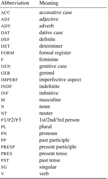
Table 5: Lexeme tag component abbreviations.
hidden Markov model (HMM) to determine which tag is correct in a given context.
Consider the following two Spanish sentences: ‘Yo como manzanas’ (‘I eat apples’) and ‘Corro como el viento’ (‘I run like the wind’). For both sentences, the FST parses the word como into the lexeme tag candidates comer.V.PRES.P1.SG ([I] eat) andcomo.ADV.CNJ(like/as). The HMM then disambiguates between the respective tags for each sentence. Table 5 contains a reference of the abbreviations used in this paper for lexeme tags.
A.2 Pimsleur and Leitner Models
As mentioned in §3.3, the Pimsleur and Leitner algorithms are special cases of HLR using fixed, hand-picked weights. To see this, consider the original practice interval schedule used by Pim-sleur (1967): 5 sec, 25 sec, 2 min, 10 min, 1 hr, 5 hr, 1 day, 5 days, 25 days, 4 months, and 2 years. If we interpret this as a sequence ofˆhΘhalf-lifes
(i.e., students should practice whenpˆΘ=0.5), we
equation. This yieldsΘ = {xn :2.4, xb :-16.5},
wherexn andxb are the number of practices and
a bias weight (intercept), respectively. This model perfectly reconstructs Pimsleur’s original schedule in days (r2 = 0.999,p0.001). Analyzing the
Leitner variant from Figure 3 is even simpler: this corresponds toΘ = {x⊕ :1, x :-1}, wherex⊕ is the number of past correct responses (i.e., dou-bling the interval), andx is the number of incor-rect responses (i.e., halving the interval).
A.3 Training and Optimization Details
The complete objective function given in§3.3 for half-life regression is:
`(hp,∆,xi; Θ) = (p−pˆΘ)2
+α(h−ˆhΘ)2+λkΘk22 .
Substituting (1) and (2) into this equation produces the following more explicit formulation:
`(hp,∆,xi; Θ) = p−2−2Θ∆·x
2
+α
−∆
log2(p)−2Θ·x
2
+λkΘk22 .
In general, the search forΘ∗weights to minimize `cannot be solved in closed form, but since it is a smooth function, it can be optimized using gradi-ent methods. The partial gradigradi-ent of`with respect to eachθkweight is given by:
∂`
∂θk = 2(ˆpΘ−p) ln 2(2)ˆp
Θ
∆ ˆ
hΘ
xk
+ 2α
ˆ
hΘ+log∆ 2(p)
ln(2)ˆhΘxk + 2λθk.
In order to fit Θ to a large amount of student log data, we use AdaGrad (Duchi et al., 2011), an online algorithm for stochastic gradient descent (SGD). AdaGrad is typically less sensitive to the learning rate parameterη than standard SGD, by dynamically scaling each weight update as a func-tion of how often the corresponding feature ap-pears in the training data:
θ(+1)k :=θk−η h
c(xk)−12
i ∂`
∂θk .
Here c(xk) denotes the number of times feature
xkhas had a nonzero value so far in the SGD pass
through the training data. This is useful for train-ing stability when ustrain-ing large, sparse feature sets (e.g., the lexeme tag features in this study). Note that to prevent computational overflow and under-flow errors, we boundpˆΘ ∈ [0.0001,0.9999]and ˆ