Munich Personal RePEc Archive
“Attitudes to Leadership and Voting:
Finding the Efficient Frontier”
Davis, Brent
Australian National University
August 2016
Online at
https://mpra.ub.uni-muenchen.de/72792/
“
Attitudes to Leadership and Voting:
Finding the Efficient Frontier
”
Dr Brent Davis
School of Politics and International Relations
Australian National University
DRAFT ONLY: COMMENTS WELCOME
August 2016
Keywords: campaigns; politimetric modelling;
Introduction
Winning elections is essentially a matter of translating the attitudes of voters into votes.
Although this proposition may sound simple, the reality is considerably more challenging
as politicians, candidates, strategists, advisers, journalists and, of course, scholars can
readily attest. A vast literature in political science, in particular in election studies, has
examined from a seemingly inexhaustible range of angles the determinants of vote choice
and the effectiveness of political campaigns across a wide field of political landscapes.
Despite the ambition, the breadth and the depth of this scholarship, a notable gap
remains: we know very little, if anything, about the efficiency with which the inputs (voter
attitudes) to the political process are converted into outputs (vote support). An
enormous number of regression models of varying design and specification focus
overwhelmingly on the effectiveness of a plethora of drivers of different outcomes in the
political process, but do not address the efficiency question. And, just because
something may be effective, it does not mean it is done efficiently, and thus done even
better.
Data Envelopment Analysis (DEA) fills this gap, providing a statistical method to
measure the efficiency with which inputs are converted into outputs. In the current
study, one of the miniscule number to examine the practical application of DEA to
political science, we look at the efficiency with which Australian political leaders and
parties have, over the past almost three decades, converted voter attitudes (approval and
disapproval) to Prime Ministers and Opposition Leaders into votes (both for their own,
and for their opponents’ parties).
The results of the DEA analysis and associated modelling find marked differences in the
political efficiency of recent Australian political leaders. Prime Ministers Hawke and
Keating had superior political efficiency in converting attitudes to political leaders into
votes, while Prime Ministers Howard and Rudd were relatively less efficient in doing so.
By contrast, Opposition Leaders Howard and Abbott appear to have been relatively
efficient in attitudes-to-vote conversion, while Opposition Leader Rudd could have
delivered the ALP an even greater winning margin in the 2007 election had he been more
Data Envelopment Analysis
DEA has its foundations, and many of its applications, in industrial economics,
management science and operations research. In essence, DEA takes quantitative
information on the inputs for/ outputs of a firm, or part thereof (for example, a number
of comparable operating units) and seeks to measure the various efficiencies with which
the firm/units convert the inputs used into outputs. DEA allows corporate and
management strategists to locate observed best practice (OBP), measure the efficiency of
the firms/units relative to OBP, and identify peers for the individual units (from which
they can seemingly learn what to do better, or not to do at all).
A simple example from public administration illustrates the point: a police command has
eight operational districts units under its control, each of which has two inputs (capital, in
the form of police cars; and labour, in the form of uniformed policemen/women), and a
single output (the ‘crime rate’, say for burglaries or shop theft). All of the inputs can be
measured, in their quantities. DEA allows senior police management to identify the most
efficient operating district, based on its combination of inputs (police cars, and
policemen/women) in producing the prescribed output (the ‘crime rate’). The efficient
frontier would be those operating district(s) which had the mix of police cars and
policemen/women which delivered the lowest crime rate (that is, OBP) for a given
combination of inputs, with the other districts measured relative to this frontier. Police
management can then look to improve the efficiency of the non-frontier districts by
examining their peer structures, and exploring reasons why some districts are at OBP and
others are behind it.
There are two general approaches to DEA: input DEA; and output DEA. Under input
DEA, the firm/unit aims to produce a given level of output with the least amount of
inputs (input minimisation); under output DEA, the firm/unit aims to produce the
greatest amount of output with a given amount of inputs (output maximisation). As a
broad statement, the private sector in most market economies focuses on input
minimisation, while the public sector would more likely adopt output maximisation given
DEA can produce a number of useful metrics of the efficiency of the firms/units under
examination. These metrics include an efficiency score, which determines which
firm(s)/unit(s) are operating at OBP and measures the distance from the other firm(s)/
unit(s) from that efficient frontier, and a scale score, which measures the effects of size of
the firm/unit on its efficiency score (larger firms/units may have economies of scale not
available to smaller firms/units). Once these metrics are known, DEA can be extended
into second-stage modelling, introducing exogenous variables into Tobit-regression
models which seek to explain the various efficiency scores. In the police resourcing case
discussed earlier, these exogenous variables might include time-of-day, season (cold vs
hot weather), school holidays, and/or the age of the local population.
Like most statistical techniques, DEA has both its strengths and weaknesses. Amongst
its strengths are DEA can: take into account both multiple inputs and outputs in a single
analysis in contrast to conventional simple regression models which are generally limited
to a single dependent variable; provide quantitative measures of technical efficiency, and
scale and allocative efficiency when size and price data are available; estimate the different
sources of inefficiency and their magnitudes; and, identify OBP operators and peers
against which the less than OBP firms/units can benchmark themselves. By contrast, its
weaknesses include: it is deterministic in nature, and thus more vulnerable to
measurement error and outliers; its sample specific, speaking only to the firms/units of
analysis at hand, and cannot necessarily be used to make more generalised statements
about a wider population; and, it only identifies which firm(s)/ unit(s) are at the efficient
frontier, and does not of itself explain why they at OBP, although this question can be
examined through DEA second-stage modelling (DEA - SSM) which can take place after
the initial DEA.
The Literature
There exists a vast literature on the theory and the applications of DEA. However,
almost all of this literature is outside of political science. While it is beyond the scope of
this study (or any other than a dedicated scholarly review) to even scratch the surface of
the general literature, DEA has had a large footprint in disciplines (and the journals
name but a few. Readily accessible studies looking at, inter alia, the application of DEA
to public administration (health services and police and corrections) in Australia, for
example, is available for non-statisticians or the non-technically inclined (PC, 1997).
By contrast, practical studies in political science using DEA are rare. To the best of our
knowledge, there appears to be just a single study (Berry and Chen (1999)) exploring the
practical application of DEA to political science. Those authors examined the efficiency
with which competing candidates converted vote intention to vote outcomes in United
States Presidential elections, demonstrating the utility of the method and supporting its
wider use in political science research. Other theoretical studies, using artificial data sets
with a political resonance, which investigate the relative merits of different DEA
methodological nuances are slightly more numerous although all come from within the
operations research rather than political science literature (Green, Doyle and Cook, 1996;
Obata and Ishii, 2003; Wang and Chin, 2007; Llamazares and Pena, 2009). But, to
reiterate, these studies were more about pushing the boundaries of DEA methodology
and theory, than about the practical application of DEA in political science.
Clearly, with the exception of just one study late last century (Berry and Chen, 1999)
there appears to be a near absence of any meaningful scholarship exploiting the potential
insights of DEA for political science in a practical manner. The next section seeks to
complement and extend the single existent offering, looking at the efficiency with which
successive Australian Governments and Oppositions have translated attitudes to party
leaders into vote intention. In short, this article in one step doubles the published
literature on the practical application o DEA to applied political science.
The Data
The data sets used in this study are taken from the regular Newspolls published by the
eponymous market research organisation. The polling data covers vote intention
(primary vote for the Australian Labor Party (ALP), and for the Liberal National Party
(LNP) coalition), and attitudes to the party leaders (their respective approval and
disapproval ratings), calculated on a monthly basis commencing in January 1986 and
opposition leaderships, producing fifteen different prime minister/opposition leader
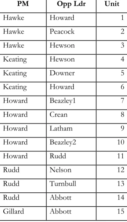
[image:7.595.192.403.160.528.2]combinations. The pattern of these combinations can be seen in Table 1.
Table 1: Australian Prime Ministers and Opposition Leaders
PM Opp Ldr Unit
Hawke Howard 1
Hawke Peacock 2
Hawke Hewson 3
Keating Hewson 4
Keating Downer 5
Keating Howard 6
Howard Beazley1 7
Howard Crean 8
Howard Latham 9
Howard Beazley2 10
Howard Rudd 11
Rudd Nelson 12
Rudd Turnbull 13
Rudd Abbott 14
Gillard Abbott 15
(ALP leaders during the period under review were Hawke, Keating and Gillard as Prime
Ministers, as well as Beazley, Crean, Latham, with Rudd as Opposition Leaders serving as
both a Prime Minister and an Opposition Leader. LNP leaders were Howard as both a
Prime Minister and an Opposition Leader, and Peacock, Hewson, Downer, Nelson,
Turnbull and Abbott) as Opposition Leaders.
The period under review covers four ALP (Hawke, Keating, Rudd and Gillard) and one
LNP (Howard) prime ministerships. Hawke, Keating and Rudd each faced three
different LNP Opposition Leaders, while Gillard confronted only one (Abbott). By
separately). Turning to Opposition Leaders, we can see Hewson, Howard and Abbott
(LNP) each confronted two different ALP prime ministers (Howard on two separate,
non-sequential occasions), while Beazley (ALP) confronted Howard (as Prime Minister)
also on two separate occasions. The longest duration of any pairing was Howard (PM)
against Beazley in his first stint as Opposition Leader (some 68 months), while the
shortest was PM Rudd against Opposition Leader Abbott (just seven months). The
variable ‘unit’ is an enumeration of the pairing, which is required for the DEA modelling
and usefully simplifies the graphics to come.
Graph 1 provides a useful first look at the relationship between the approval and the
disapproval ratings for the LNP leader, while Graph 2 does the same for the ALP leader.
Recall: observation 1 is the scatter dot point for PM Hawke/Opp Ldr Howard,
observation 2 is for PM Hawke/ Opp Ldr Peacock, and so on, as reported in Table 1.
Graph 1: Approval and Disapproval for LNP Leader
The best net approval (approval/disapproval) situation for an LNP leader, regardless of
office held, was during the PM Howard/ Opp Ldr Crean period (observation 8), with a
ratio of 1.56 times (that is, Howard’s approval rating was 1.56 times his disapproval rating), closely followed by PM Howard/ Opp Ldr Latham (observation 9; ratio = 1.46
times). By contrast, the worst net approval situation for an LNP leader was the PM
1 2 3 4 5 6 7 8 9 10 11 12 13 14 15 20 25 30 35 40 45 50 55
20 25 30 35 40 45 50 55 60
DSL NP, P e r ce n t
APLNP, Per cent
Hawke/Opp Ldr Peacock period (observation 2; ratio = 0.45 times), followed closely by
PM Hawke/Opp Ldr Howard (observation 1; ratio = 0.59 times). Interestingly, Opp
Ldr Abbott experienced a substantial net disapproval rating (observation 15; ratio = 0.67
times) during the period under review when he was up against PM Gillard, but he
(Abbott) still went on to win the subsequent federal election. As a visual inspection of
Graph 1 indicates, and as would be expected, there was a clear negative correlation
between approval and disapproval ratings for the LNP leader (r = -0.683; t = -3.37; p =
0.01).
Graph 2: Approval and Disapproval for ALP Leader
The best net approval situations for an ALP leader, again regardless of office held, were
those where Kevin Rudd was Opposition Leader against Prime Minister Howard
(observation 11; ratio = 3.44), followed by when Rudd was Prime Minister against
Opposition Leaders Nelson (observation 12; ratio = 2.78) and Turnbull (observation 13;
ratio = 2.29). The worst net approval situation for an ALP leader was PM Keating
against Opp Ldr Hewson (observation 4; ratio = 0.55), and PM Keating against Opp Ldr
Howard (observation 6; ratio = 0.60). Again, there was a clear and negative correlation
between approval and disapproval for ALP leaders (r = -0.941; t = -10.01; p = 0.00).
1 2 3 4 5 6 7 8 9 10 11 12 13 14 15 10 15 20 25 30 35 40 45 50 55 60
20 30 40 50 60 70
DEA Analysis
Identifying the efficient frontier for the conversion of party leader approval and
disapproval ratings into vote support – the core interest of DEA – can be undertaken in
a two-step process. The first step, again, involves the use of scattergrams, being modified
forms of Graphs 1 and 2 reported earlier, with the second step involving dedicated DEA
modelling. The scattergrams have to be reconfigured, however, with the axes normalised
by dividing the approval or disapproval scores by their respective vote intention scores
(eg approval for LNP leader/ vote intention for LNP party). The efficient frontier is
likely to be found where the party leader has the lowest disapproval-to-vote-intention,
and the highest approval-to-vote-intention ratios. Graph 3 reports a scattergram of
where the efficient frontier may lay for the LNP leader/party, while Graph 4 does the
same for the ALP leader/party.
Graph 3: The LNP Frontier
The efficient frontier for the LNP leader/ party is the vertical line rising from
observation 15, the diagonal line connecting observations 15 and 2, and the horizontal
line running from observation 2. As such, the most efficient LNP leaders appear to be
Opp Ldr Abbott (against PM Gillard: observation 15), and Opp Ldr Peacock (against PM
1 2 3 4 5 6 7 8 9 10 11 12 13 14 15 50 60 70 80 90 100 110 120 130 140
60 70 80 90 100 110 120 130
Hawke: observation 2), although Opp Ldr Downer (against PM Keating: observation 5)
appears to sit close to the LNP’s efficient frontier. By contrast, the least efficient LNP leaders were PM Howard when up against Opp Ldr Rudd (observation 11), and Opp
Ldrs Nelson (observation 12) and Turnbull (observation 13) against PM Rudd.
Interestingly, then Opp Ldr Abbott (against PM Gillard) essentially shifted the efficient
frontier for the LNP (the connecting line between observations 15 and 2), away from the
previous frontier connecting observations 2, 5, 4 and 3 – being LNP leaders Peacock,
Downer, Hewson and Hewson, respectively).
Graph 4: The ALP Frontier
The efficient frontier for the ALP leader/party is likely to be found at the vertical line
rising from observation 4, the diagonal lines connecting observations 4 and 8, and 8 and
11, and then the horizontal line running from observation 11. The most efficient ALP
leaders appear to be PM Keating (against Opp Ldr Hewson: observation 4; and
potentially against Opp Ldr Downer: observation 5), Opp Ldr Crean (against PM
Howard; observation 8), and Opp Ldr Rudd against PM Howard (observation 11). In
general terms, Keating and Crean may have done well in minimising the adverse impact
of their relatively high disapproval ratings, while Rudd did well in maximising the positive
impact of his relatively high approval rating, on ALP vote intention.
1 2 3 4 5 6 7 8 9 10 11 12 13 14 15 30 50 70 90 110 130 150 170
60 80 100 120 140 160
Three DEA models where specified: the first examined the impact of approval ratings for
party leaders on votes for the two parties (that is, approval for the LNP leader and
approval for the ALP leader, on vote for the LNP and vote for the ALP: aplnp, apalp →
vlnp, valp; DEA allows both multiple explanatory and dependent variables); the second
replicated the first, except using disapproval ratings for the leaders (dslnp, dsalp → vlnp,
valp); and, the third used the net approval (that is, approval divided by disapproval)
ratings for the party leaders, on vote for each of the two parties (netlnp, netalp → vlnp,
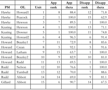
valp). Table 2 summarises the results for the first two models (approvals and disapprovals,
[image:12.595.108.488.343.659.2]on vote intention).
Table 2: Efficient Frontier :
Approvals and Disapprovals, and Vote Intention
App App Disapp Disapp PM OL Unit rank theta rank theta
Hawke Howard1 1 8 88.4 12 71.8
Hawke Peacock 2 1 100.0 15 62.9
Hawke Hewson 3 7 89.5 1 100.0
Keating Hewson 4 1 100.0 13 71.1
Keating Downer 5 1 100.0 11 74.8
Keating Howard2 6 4 96.3 6 91.4
Howard Beazley1 7 11 72.9 8 85.6
Howard Crean 8 5 92.1 5 91.6
Howard Latham 9 15 63.7 1 100.0
Howard Beazley2 10 9 82.9 10 81.0
Howard Rudd 11 13 69.5 1 100.0
Rudd Nelson 12 10 76.6 1 100.0
Rudd Turnbull 13 12 70.0 7 88.6
Rudd Abbott 14 14 69.0 9 81.1
Gillard Abbott 15 6 90.7 14 67.5
Looking first at the approval DEA scores, the efficient frontier (the combinations of
political leaders most efficient in translating approval ratings into vote intentions – those
intention (those with the lowest theta’s) were Howard/Latham, Rudd/Abbott, and
Howard/Rudd, with an average theta of 67.3 per cent (that is, almost 33 per cent behind
the efficient frontier). Turning to the disapproval DEA scores, the efficient frontier (the
most efficient at translating disapprovals into vote intention) were Hawke/Hewson,
Howard/Latham, Howard/Rudd and Rudd/Nelson, while the least efficient at doing so
were Hawke/Peacock, Gillard/Abbott and Keating/Hewson, with a theta average of
67.2 per cent (or around 33 per cent behind the efficient frontier). The average of the
approvals and the disapproval thetas were essentially the same (84.1 per cent and 84.5 per
cent), while the standard deviations were almost identical (12.8 per cent respectively),
implying no statistically significant differences between the means for the two series.
Nevertheless, any political practitioner would likely quickly point out while it is
interesting to examine approvals and disapprovals separately for the efficiency with which
they are translated into vote intention, the better approach is to combine both into a
single model. That is, the efficient vote intention frontier for both parties is formed by
taking into account both approval and disapproval for both party leaders. Regrettably,
there are insufficient observations (n = 15) to sustain a specification containing all four of
the explanatory variables (aplnp, apalp, dslnp and dsalp), although when reduced to net
approval for the LNP leader (netlnp = aplnp/dslnp) and for the ALP leader (netalp =
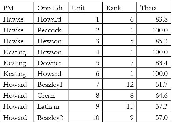
[image:13.595.161.436.560.757.2]apalp/dsalp) such modelling can proceed. The results of such modelling are reported in
Table 3.
Table 3: Efficient Frontier : Net Approval and Vote Intention
PM Opp Ldr Unit Rank Theta
Hawke Howard 1 6 83.8
Hawke Peacock 2 1 100.0
Hawke Hewson 3 5 85.3
Keating Hewson 4 1 100.0
Keating Downer 5 7 83.4
Keating Howard 6 1 100.0
Howard Beazley1 7 12 51.7
Howard Crean 8 8 64.6
Howard Latham 9 15 37.3
Howard Rudd 11 11 52.5
Rudd Nelson 12 13 48.4
Rudd Turnbull 13 14 45.0
Rudd Abbott 14 10 54.0
Gillard Abbott 15 4 91.2
The Hawke/Peacock, the Keating/Hewson and the Keating/Howard combinations were
at the efficiency frontier for translating net approval ratings for the party leaders into vote
intentions, while Gillard/Abbott were not far behind. In a manner, this result is not all
that surprising, given the tendency for at least three of the party leaders (Keating, Gillard
and Abbott) to have been regarded as ‘hard ball political players’. By contrast, the least
efficient (farthest behind the efficient frontier) were Howard/ Latham (37.3 per cent, the
latter having a reputation as something of a ‘policy wonk’), Rudd/Turnbull (45 per cent)
and Rudd/Nelson (48.4 per cent), again when Rudd was seen as a ‘bookish nerd’.
Second Stage Modelling
While it is possible to speculate on possible drivers of these different efficiency profiles
and locations, DEA modelling per se only tells us ‘who sits where’ on and relative to the
efficiency frontier; of itself, it does not answer the inevitable question of ‘why’ –“why do
the parties/leaders have different locations on/relative to the efficient frontier?”
However, so-called ‘second stage modelling’ provides a platform for such investigation,
using tobit regression, with the theta results from the DEA modelling used as the
dependent variables, along with exogenous political variables likely to cause those
efficiency scores.
The exogenous variables used in the second stage modelling are dummy variables for the
individual Prime Ministers (being equal to one when the person was Prime Minister, and
zero otherwise), thus seeking to identify a ‘prime ministerial effect’. As such, we are
asking ‘were there practical and statistically significant differences in the efficiency of
translating voter approval and disapproval ratings into vote intention across the different
prime ministers?’. The results of this second stage modelling are reported in Table 4.
The dependent variable is the theta scores for each Prime Minister/ Opposition Leader
equal to one when Hawke was Prime Minister, and zero otherwise; in the Keating Model
it would be equal to one when Keating was Prime Minister, and zero otherwise; and so
on; assuming the prime minister sets the political agenda, and the political tone during
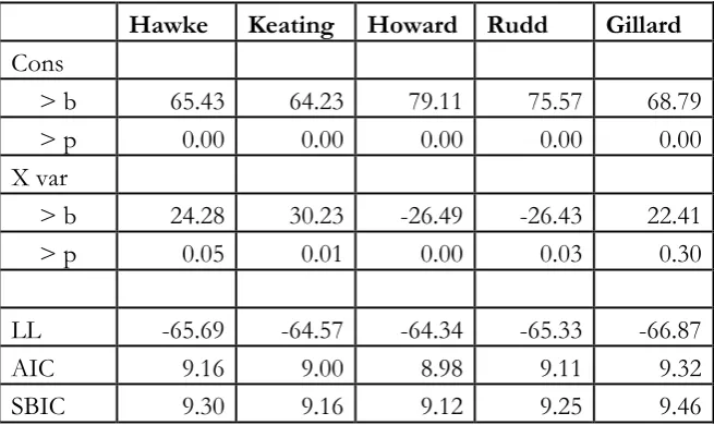
[image:15.595.134.462.201.396.2]their incumbency.
Table 4: Second Stage Modelling: Prime Ministers
Hawke Keating Howard Rudd Gillard
Cons
> b 65.43 64.23 79.11 75.57 68.79
> p 0.00 0.00 0.00 0.00 0.00
X var
> b 24.28 30.23 -26.49 -26.43 22.41
> p 0.05 0.01 0.00 0.03 0.30
LL -65.69 -64.57 -64.34 -65.33 -66.87
AIC 9.16 9.00 8.98 9.11 9.32
SBIC 9.30 9.16 9.12 9.25 9.46
Looking at the parameter coefficient’s for the prime ministerial dummy variables indicates the presence of Paul Keating as prime minister had the greatest marginal impact
on the efficiency with which voter attitudes to the political leaders were translated into
votes (b = 30.2; p = 0.01) when compared to the other prime ministers, which is not all
that surprising given the highly charged political environment in which Keating operated
(either by circumstance, or by his own political design). By contrast, Howard and Rudd
both appear to have been relatively less efficient than their prime ministerial peers in
translating voter attitudes to political leaders into vote intention (b = -26.49; p = 0.00;
and, b = -26.43; p = 0.03, respectively).
A similar exercise can be undertaken looking at the efficiency effects of different
opposition leaders. However, given there were 11 different opposition leaders across the
period under review, a simple replication of the prime ministerial is likely to prove
tedious, and potentially generate more noise than light. As such, we will focus our
attention on the three opposition leader periods where the Leader concerned won
Abbott, defeating Gillard), and the special case of Latham vs Howard (for the standout
[image:16.595.163.435.179.393.2]nature of the former’s political personality). The analytical approach is the same as for the prime ministers; results for these second stage models are reported in Table 5.
Table 5: Second Stage Modelling: Opposition Leaders
Howard Rudd Abbott Latham
Cons
> b 68.16 71.55 68.79 72.64 > p 0.00 0.00 0.00 0.00 X var
> b 31.84 -19.50 22.41 -35.34 > p 0.13 0.38 0.30 0.08
LL -66.30 -67.01 -66.87 -66.02
AIC 9.24 9.34 9.32 9.20
SBIC 9.38 9.47 9.46 9.34
Looking first at the results for the Howard, Rudd and Abbott models (that is, those
opposition leaders who subsequently won office, to become prime ministers), the stand
out message is while the two LNP Leaders (Howard and Abbott) added to the political
efficiency of attitude-to-vote transfer, while Rudd (ALP) diminished efficiency, none of
these results were statistically significant at conventional levels; they could have been due
to chance alone. By contrast, the Latham incumbency as Opposition Leader saw a
substantial fall away in the relative efficiency of attitude-to-vote transfer, a result which
was close to statistical significance (b = -35.34; p = 0.08).
Conclusion
DEA provides a very useful mechanism for assessing the efficiency with which political
parties are able to harvest voter attitudes to political leaders, both the approval and
disapproval of ‘our’ and ‘their’ leader on ‘our’ and ‘their’ votes. It enables political
scholars and strategists to measure the electoral importance of positive (working to
Used strategically, DEA allows scholars and strategists to identify the efficient frontier
for, in this case, the conversion of attitudes to political leaders to vote support, locate
where ‘our’ and ‘their’ leaders are relative to this efficiency frontier, and use accessible
modelling techniques to get insights as to what might have to be done to get to that
frontier. The seeming paucity of scholarly articles applying DEA to political science, is
for this reason alone, somewhat surprising; but, we have at least attempted to fill the gap.
In the current context, it would appear Hawke and Keating were political assets for their
parties (in both cases, the ALP) in their superior efficiencies in translating attitudes to
political leaders into votes, with Howard and Rudd being much less efficient. As such,
Hawke and Keating likely delivered their respective governments larger than otherwise
vote outcomes, and hence number of seats in Federal Parliament, while Howard and
Rudd did the opposite (lower than otherwise vote outcomes, and less than otherwise
seats). Gillard appears to have had no real impact either way.
By contrast, the capacities of Howard and Abbott as opposition leaders to increase the
efficiency of attitude-to-vote transfer likely helped their political parties (in both cases,
the LNP) to win greater than otherwise vote outcomes which in turn likely meant
higher-than-otherwise number of seats in the federal election which saw them elected to the
prime ministerships. By contrast, Rudd as opposition leader appears to have subtracted
from the ALP’s vote performance, in the sense that while they won the 2007 federal
election, they could have done even better still. Latham, to put it nicely, was ‘sand in the wheels of the ALP’, at least in terms of efficiency in converting attitudes to political
leaders into votes.
Bringing it all together, it would appear Hawke and Keating (both ALP leaders) are case
studies of what Prime Ministers and their advisers need to do to efficiently convert
attitudes to political leaders into vote, while Howard and Abbott (both LNP leaders) are
similarly positioned for Opposition Leaders. By contrast, Howard and Rudd as Prime
Bibliography
Berry B J L and Chen Y-S (1999) “Measurement of Campaign Efficiency Using Data
Envelopment Analysis” 18 Electoral Studies 379 – 395
Green R H, Doyle J R and Cook W D (1996) “Preference Voting and Project Ranking
Using DEA and Cross-Evaluation” 90 European Journal of Operational Research 461 –
472
Llamaszares B and Pena T (2009) “Preference Aggregation and DEA: An Analysis of the
Methods Proposed to Discriminate Efficient Candidates” 197 Journal of European
Operational Research 714 – 721
Obata T and Ishii H (2003) “A Method for Discriminating Efficient Candidates With
Ranked Voting Data” 151 Journal of European Operational Research 233 - 237
Productivity Commission (1997) “Data Envelopment Analysis: A Technique for
Measuring Efficiency in Government Service Delivery”, Productivity Commission,
Canberra
Wang Y-M and Chen K-S (2007) “Discriminating DEA Efficient Candidates by
Considering Their Least Relative Total Scores” 206 Journal of Computational and