Stock Return Prediction with Fully Flexible Models and Coefficients

Munich Personal RePEc Archive

Stock Return Prediction with Fully

Flexible Models and Coefficients

Byrne, Joseph and Fu, Rong

Department of Accountancy, Economics and Finance, Heriot-Watt

University

9 November 2016

Stock Return Prediction with Fully Flexible Models and

Coefficients

Joseph P. Byrne ∗† Rong Fu ∗

November 9, 2016

Abstract

We evaluate stock return predictability using a fully flexible Bayesian framework,

which explicitly allows for different degrees of time-variation in coefficients and in

fore-casting models. We believe that asset return predictability can evolve quickly or slowly,

based upon market conditions, and we should account for this. Our approach has superior

out-of-sample predictive performance compared to the historical mean, from a

statisti-cal and economic perspective. We also find that our model statististatisti-cally dominates its

nested models, including models in which parameters evolve at a constant rate. By

de-composing sources of prediction uncertainty into five parts, we find that our fully flexible

approach more precisely identifies time-variation in coefficients and in forecasting models,

leading to mitigation of estimation risk and forecasting improvements. Finally, we relate

predictability to the business cycle.

JEL classification: C11,G11, G12, G17

Keywords: Stock return prediction, Time-varying coefficients and forecasting

mod-els, Bayesian econometrics, Forecast combination

∗_{Heriot-Watt University, Department of Accountancy, Economics and Finance, Edinburgh, EH14 4AS, UK.}

1

Introduction

Stock return predictability continues to be a core area of research in financial economic.

This research is often skeptical about standard models or predictors and their out-of-sample

forecasting power (Goyal and Welch, 2003; Cooper and Gulen, 2006; Andrew and Geert, 2007;

Campbell and Thompson, 2008; Welch and Goyal, 2008; Joscha and Sch¨ussler, 2014; Turner,

2015). For instance, Welch and Goyal (2008) comprehensively investigate the predictive power

of commonly used asset pricing indicators: these predictors only occasionally have a good

out-of-sample performance. Predictive power improves for some predictors in specific periods

of stress, suggesting the presence of both model uncertainty and instability. In this paper,

therefore, we investigate whether flexibly accounting for model uncertainty and parameter

instability, can improve stock return prediction.

The literature agrees that ignoring model uncertainty and instability impairs

predictabil-ity (Stambaugh, 1999; Wachter and Warusawitharana, 2009; Dangl and Halling, 2012; Billio

et al., 2013; Johannes et al., 2014; Wachter and Warusawitharana, 2015). Time-varying

pa-rameters in predictive regressions have been previously considered in the literature. Bossaerts

and Hillion (1999) argue that the poor out-of-sample performances of the prediction models

is due to model nonstationarity: in other words, the parameters of the model should be

time-varying. Similarly, by splitting the whole sample into different subsample periods, Andrew

and Geert (2007) clearly find evidence of time-evolving parameters.

In addition to the problem of parameter instability, a large array of excess stock return

predictors has been identified in the literature. Therefore, how to combine from a range

of predictors to forecast stock returns should also be considered. This is known as model

uncertainty. Stock return determinants and hence forecasting models may also change at

each time period, as demonstrated in Avramov (2002), Cremers (2002), Rapach et al. (2010),

Dangl and Halling (2012) and Johannes et al. (2014). Specifically, Johannes et al. (2014)

argue that incorporating different model features, such as time-evolving expected returns,

time-varying volatility and taking account of estimation error, is beneficial for out-of-sample

gains.

accuracy, the exact nature of time-variation in parameters and how to accommodate model

uncertainty may matter for prediction. To successfully predict excess stock returns, we tackle

these issues in this paper. Our main aim is try to answer the following research questions: Is

time-variation in coefficients and in forecasting models rapid or do they evolve more slowly?

How important is the problem of model uncertainty and parameter instability for stock return

predictability?

Bayesian methods are reasonable to answer these questions, for instance the approaches

of Raftery et al. (2010) and Koop and Korobilis (2012), since they take parameter

instabil-ity and model uncertainty into account. These Dynamic Model Averaging (DMA) methods

assume that coefficients and forecasting models vary in the same fashion over time.

Harri-son and West (1999) suggest that the fixed dynamics for evolution is unappealing and some

model specifications can only be appropriate for some periods. For example, investors may

rapidly update the relative importance of equity predictors in times of market stress and

less rapidly in other times. We consider whether the assumption of Raftery et al. matters

when predicting returns. In this sense, we construct Dynamic Mixture Model Averaging

(DMMA), which allows for possible degrees of time-variation in coefficients and forecasting

models, nesting gradual to abrupt changes in coefficients. In the extreme, our DMMA

ap-proach even accommodates constant coefficients and equal model weights. This implies our

model is sufficiently flexible to detect and exploit locally appropriate forecasting models over

time. In this framework, we can identify which predictors, which degrees of time-variation in

coefficients and forecasting models result in better stock market predictability.

Our contribution goes further than constructing DMMA and comparing its out-of-sample

performances to alternative models. The added flexibility of our DMMA approach allows

us to analyze what leads to forecasting improvements. We can investigate whether forecast

improvements are due to different predictors, different degrees of time-variation in coefficients

and forecasting models. To that end, we decompose prediction variance into five parts: (i)

model uncertainty caused by random fluctuations in the data process (observational

vari-ance), (ii) uncertainty due to the errors from estimating the coefficients (estimation risk),

(iii) model uncertainty with respect to predictor selection, (iv) model uncertainty regarding

of different choices of the magnitude of time-variation in forecasting models. To the best of

our knowledge, this is the first stock paper that systematically examines the role of model

uncertainty in terms of different degrees of time-variation in forecasting models.

Methodologically, the paper most similar to ours is Dangl and Halling (2012), which takes

parameter instability as well as model uncertainty into account, by employing time-varying

coefficients with Bayesian Model Averaging (BMA) using macroeconomic predictors.

How-ever, our paper extends theirs in the following regards. First, the widely used Bayesian Model

Averaging (BMA) method (Avramov, 2002; Cremers, 2002; Dangl and Halling, 2012; Turner,

2015) combines different models recursively according to posterior model probabilities.

How-ever, BMA does not distinguish the difference between the more recent forecast performance

and the more distant past forecast performance. Even though Dangl and Halling (2012)

employ recursive forecasting and incorporate some time variation in the forecasting model,

posterior model probabilities will only vary slightly as new data is incorporated. Whereas,

for DMA, recent forecast performance receives a higher weight. This allows for more rapid

changes for different forecasting models’ posterior weights. Our DMMA approach is flexible

enough to encompass both DMA and BMA. It even allows for models with equal weights.

Hence, DMMA is advantageous in embedding the locally proper degree of time-variation in

forecasting models at each time. Moreover, we not only consider the macroeconomic

predic-tors emphasized by Dangl and Halling (2012), but also technical predicpredic-tors used in a recent

paper by Neely et al. (2014), providing complementary information about the stock market.

Beside, we use stochastic volatility instead of the constant volatility employed in Dangl and

Halling (2012), which accommodates the widely identified fat tail property of financial data.

Finally, compared with Dangl and Halling (2012), we add one more element of model

uncer-tainty: uncertainty with regard to different choices of time-variation in forecasting models,

and we study what leads to forecast improvements according to different sources of

uncer-tainty.

To preview our results, we find that our Dynamic Mixture Model Averaging (DMMA)

predominately outperforms the historical mean (HM), with positive out-of-sample R2

and

large utility gains relative to historical mean for a mean-variance investor across different

in-cluding equal weights, Bayesian Model Averaging (BMA) and Dynamic Model Averaging

(DMA), in terms of point forecast accuracy. We also find that imposing constant coefficient

on predictive models worsens out-of-sample performance. The reason why DMMA performs

better than its nested models is that by detecting the locally appropriate time-variation in

co-efficients and in forecasting models, DMMA alleviates the problem of model misspecification,

leading to forecast improvements.

Importantly, we further analyze different sources of uncertainty for different predictive

model. Regarding DMMA, observational variance, model uncertainty with respect to

predic-tor selection and uncertainty regarding the errors from estimating the coefficients are the top

three obstructing factors in forecast performance. In contrast, uncertainty about the degree

of time-variation in coefficients is small and uncertainty regarding the degree of time-variation

in forecasting models only appears in the initial data points. This suggests that DMMA

suc-cessfully adapts to stock market instability by embedding the precise level of time-variation

in coefficients and forecasting models. Interestingly, when we fix the variability in coefficients

and in forecasting models, the percentage weight of estimation error is large. The flexible

DMMA, in contrast, has small estimation risk. As a consequence, one possible

explana-tion for DMMA’s superior out-of-sample performance is that considering a possible range of

time-variation in coefficients increases coefficient variability, and offsets the loss in forecast

accuracy caused by the coefficients estimation uncertainty. In addition, by allowing for

dif-ferent degrees of time-variation in forecasting models, we flexibly enhance model adaptability

and quickly detect locally appropriate models, therefore, further compensate the losses due

to estimation risk.

Linking DMMA’s predictability to the business cycle, we find that DMMA has superior

out-of-sample performances during recessions than expansions. DMMA also outperforms HM

statistically and economically during all the expansions. Importantly, the predicted equity

premium increases at the end of recessions and decreases when the recessions start. This is

consistent with the asset pricing theory in the literature (Fama and French, 1989; Campbell

and Cochrane, 1995; Cochrane, 1999, 2005; Rapach et al., 2010; Dangl and Halling, 2012).

Hence, the investor who follows DMMA perfectly times the stock market. The agreement

premium predictability.

2

Econometrics Framework

In this section we set out our approach to excess return prediction, while accommodating

three dimensions of model uncertainty: different predictor selection, different degrees of

time-variation in coefficients and different degrees of time-time-variation in forecasting models. This

flexible prediction framework takes different sources of uncertainty into account. Specially, in

Section 2.1, we demonstrate a dynamic linear model which allows for time-varying coefficients

for a certain choice of predictors. In Section 2.2, we construct the Dynamic Mixture Model

Averaging method to attach posterior probabilities to individual models that have alternative

predictors and different degrees of time-variation in coefficients. Then combine individual

models together using different degrees of time-variation in forecasting models.

2.1 Dynamic Linear Model

Consistent with the majority of research on stock return prediction, we assume a linear

prediction model (Avramov, 2002; Cremers, 2002; Andrew and Geert, 2007; Welch and Goyal,

2008; Dangl and Halling, 2012; Joscha and Sch¨ussler, 2014). Moreover, our model allows for

time-variation in the coefficients of the prediction model. As Dangl and Halling (2012)

acknowledge, by reducing estimation errors and calibrating coefficients to observed data,

random-walk coefficients have better out-of-sample performances compared to autocorrelated

coefficients.1

In light of this, we allow the time-varying coefficients to follow a random walk

process, signalling that changes in coefficients are unpredictable. Note that our prediction

and out-of-sample performance are in real time: we only use information at or before timet

if we want to predict the excess stock return att+ 1.

Particularly, assumertis the expected stock returns at timet,Xt−1is the specific predictor

for each individual model at timet−1 and time-varying parameter models are allowed. We

1

perform the return prediction on a monthly basis.

rt=Xtθt+εt, εt∼N(0, Ht) (observation equation) (1)

θt=θt−1+ut, ut∼N(0, Qt) (transition equation) (2)

where the errorsεtandutare normally distributed with zero mean and uncorrelated across all

lags with time-varying variancesHtandQt, respectively. We refer toHtas the observational

variance in the following; Xt = [1, xt−1], where xt is the single predictor we choose at time

t. Therefore, dynamic linear models differ with respect to the choices of predictors. In the

Section 3.1, we discuss the set of predictors inxt.

Given that we take a Bayesian perspective, denoteDt= [rt, rt−1, . . . , Xt, Xt−1, . . . , P riors]

as the information set available att, which includes all the previous information about excess

stock return values, predictor values, as well as the priors for coefficientsθ0and observational

varianceH0. Essentially, we use a simple Kalman filter, following Raftery et al. (2010) and

Koop and Korobilis (2012), to incorporate forgetting factors into the evolution of the

parame-ters to capture the dynamics of the estimated coefficients and reduce the large computational

burden. To explain how it works, start from the standard Kalman filter. We can obtain

the posterior distribution for θt−1 as ut follows a normal distribution with mean zero and

covarianceQt:

θt−1|Dt−1 ∼N(ˆθt−1,Σt−1_|t−1) (3)

Kalman filter predicts θt conditional on the information up to timet−1:

θt|Dt−1 ∼N(ˆθt−1,Σt|t−1) (4)

Σ_t|t−1= Σt−1|t−1+Qt (5)

Raftery et al. (2010) and Koop and Korobilis (2012) suggest using a form of forgetting

to ease computational demands in stead of specifying the matrixQt. In particular, equation

(5) is replaced by:

Σ_t|t−1 =

1

where λ is the forgetting factor and 0 < λ ≤ 1. Therefore, according to equation (6),

the forgetting factor λis essential in influencing the degree of time-variation in coefficients.

Effectively, the forgetting factor λ can be interpreted as the age-weights for different time

point, thus, the effective window size used for estimation is 1/(1−λ). For example, settingλ=

1 means that the covariances of coefficients, Σt|t−1are constant over time, thus, the coefficients

themselves are constant over time. This also implies that a constant-coefficients predictive

model is nested in equation (1). Whereas, settingλ <1 implies that the covariances, Σ_t|t−1

increase over time and coefficients are time-varying. Moreover, the lower the value of λs,

the more abrupt the coefficients change. If we assumeλ=0.99 with monthly data, it means

that observations for the covariances of coefficients, Σt|t−1, last year has approximately 89%

as much weight as last month. This is therefore the case when we have gradually changing

coefficients. When the coefficients change suddenly, with λ=0.90, observations one year ago

only account for 28% as much weight as last month’s. This implies that λ has substantial

influence on coefficient stability and different degrees of λ lead to different dynamic linear

models.

In the appendix, we provide details on the predictive distribution and time-varying

volatil-ity.

2.2 Dynamic Mixture Model Averaging

In Section 2, we argued that different predictors and degrees of time-variation in

coef-ficients may influence our ability to forecast stock returns. Improper model selection can

increase total variance of return prediction and affect the accuracy of statistical inference.

However, one specification from the substantial pool is unlikely to dominate all others at

each point in time. Since a single model may not be systematically the most successful at

prediction, one potential approach is to take model uncertainty into account and compare

all the models simultaneously. Dynamic Model Averaging (DMA) allows for time-varying

coefficients and weights attached to each model changing over time based upon their past

forecasting performances (Raftery et al., 2010; Koop and Korobilis, 2012). However, Raftery

et al. (2010) and Koop and Korobilis (2012) assume ex-ante that coefficients in the predictive

we construct Dynamic Mixture Model Averaging (DMMA) to allow for possible degrees of

time-variation in coefficients and forecasting models, nesting gradual to abrupt change, and

even constant coefficients and forecasting models. Therefore, in addition to the uncertainty

about the choice of the predictors, we consider two more model uncertainties compared to

Raftery et al. (2010) and Koop and Korobilis (2012): uncertainty regarding different degrees

of time-variation in coefficients and in forecasting models. Using a Bayesian approach, the

data identifies the precise degree of time-variation in coefficients and forecasting models by

attaching posterior weights to possible models. This flexibility allows us to detect locally

proper models over time.

In general, DMA suggests that the degrees of time-variation for coefficients and

fore-casting models are controlled by two forgetting factors. The first forgetting factor is the λ

we mentioned above, which controls the degree of time-variation in coefficients. The other

forgetting factor isα, which controls the degree of time-variation in forecasting models and

will be explained later. Particularly, denoteki a choice of predictors fromK candidates,λj a

choice of time-variation in coefficients fromdcandidates andαz a choice of time-variation in

forecasting models fromacandidates. Then, there are d·K possible dynamic linear models

and a different ways of combining them. Consequently, the predictive density of individual

models and final forecasting results depends on the selection of predictors (ki), degrees of

time-variation in coefficients (λj) and degrees of time-variation in forecasting models (αz) as

well. Further details on the model combination are available in the appendix.

Note that the prediction equation for different variables can be written in the form of

conditional predictive density, thus, the predictive weight attached to each variableki is :

P(Lt=ki |λj, αz, Dt−1)∝[P(Lt−1=ki |λj, αz, Dt−2)P(rt−1|Lt−1 =ki, λj, αz, Dt−2)]αz

=

t−1 Y

s=1

[P(rt−s|Lt−1 =ki, λj, αz, Dt−s−1)]α

s z

(7)

whereLt represents the model selected at timet.

Therefore, if the predictive density for variable ki conditional on the degree of

more weight at time t, which is controlled by the forgetting factor α. If a certain value is

allowed for α, it might only be locally suitable and the model can be misspecified. Our

task is to make the model averaging process as flexible as possible and allow data to detect

appropriate models by considering different degrees ofα.

Interestingly, some conventional models are nested in DMMA. When models are equally

weighted, α = 0, forecasting models are constant over time. Huang and Lee (2010) suggest

equal weights dominates other forecasting methods, using equity premium prediction as an

example. Similarly, Rapach et al. (2010) demonstrate the superior out-of-sample equity

pre-mium prediction of equal weights combination method. Whenα= 1, there is no discounting,

and therefore, no role for α, model averaging shrinks to normal BMA. BMA, the approach

widely widely used in the stock return prediction literature (see for example Avramov (2002);

Cremers (2002); Dangl and Halling (2012) and Turner (2015)), equally weights all the data

from the more distant past and the more recent past. When α < 1, model weights are

time-varying. For instance, ifα = 0.99, given monthly data, forecast performance last year

receives 89% weight compared to that last month, which is a gradual change. Whereas, if

α= 0.90, 89% abruptly changes to 28%.

The posterior probability of eacha·d·K specification is updated according to Bayes rule.

In the appendix, we provide more details about Dynamic Mixture Model Averaging.

3

Empirical study design

3.1 Data description

We examine stock predictability using monthly data of the S&P 500 index excess returns,

and in particular the difference between monthly return on the stock market and the risk-free

rate. The choice of predictors is guided by the literature. In particular, numerous research

relies on macroeconomic predictors to forecast equity premium while paying little attention

to technical indicators. Neely et al. (2014), however, address the fact that macroeconomic

predictors and technical indicators provide complementary information in terms of improving

forecast accuracy and economic gains. Therefore, we consider macroeconomic predictors as

The macroeconomic predictors we apply are the most widely used in empirical excess

returns models.2

Therefore we use the data set from Welch and Goyal (2008).3

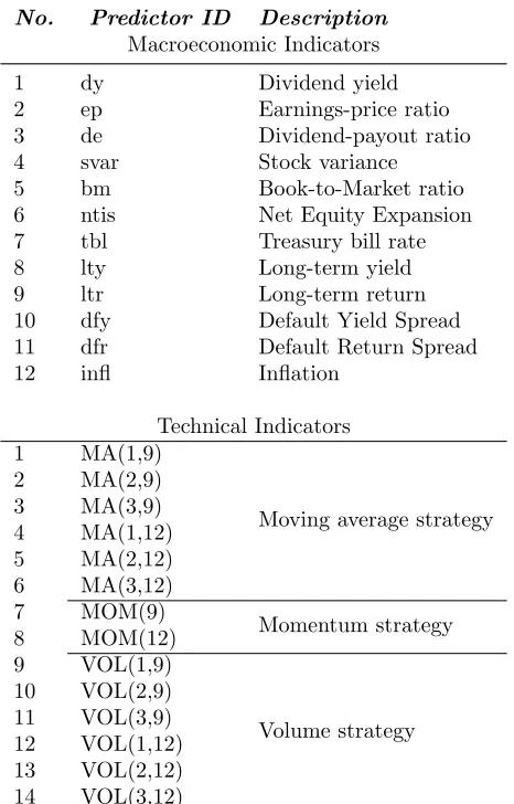
Table 1

provides a short description of 12 macroeconomic predictors4

for the sake of brevity (see

Welch and Goyal (2008) for details).

Table 1: List of Predictors

No. Predictor ID Description

Macroeconomic Indicators

1 dy Dividend yield

2 ep Earnings-price ratio

3 de Dividend-payout ratio

4 svar Stock variance

5 bm Book-to-Market ratio

6 ntis Net Equity Expansion

7 tbl Treasury bill rate

8 lty Long-term yield

9 ltr Long-term return

10 dfy Default Yield Spread

11 dfr Default Return Spread

12 infl Inflation

Technical Indicators

1 MA(1,9)

Moving average strategy

2 MA(2,9) 3 MA(3,9) 4 MA(1,12) 5 MA(2,12) 6 MA(3,12) 7 MOM(9) Momentum strategy 8 MOM(12) 9 VOL(1,9) Volume strategy 10 VOL(2,9) 11 VOL(3,9) 12 VOL(1,12) 13 VOL(2,12) 14 VOL(3,12)

Notes: This tables shows the description of macroeconomic and technical predictors. Data is from De-cember 1950 to DeDe-cember 2015.

Following Neely et al. (2014), we also construct 14 technical predictors based on three

2

Some powerful macroeconomic predictors are uncovered, including net payout yield (Boudoukh et al., 2007), investor sentiment aligned (Huang et al., 2015) and short interest (Rapach et al., 2016). All of them are suggested to have comparably good out-of-sample performances. However, in our paper, we exclude these predictors due to data availability.

3

The data are available from Amit Goyal’s webpage at http://www.hec.unil.ch/agoyal/.

4

strategies: moving-averages (MA), momentum (MOM) and volume (VOL). Table 1 illustrates

the technical predictors we consider.5

MA(s, l) generates a buy signal if the stock price in

the short(s) MA is larger than that in the long(l) MA (s= 1,2,3 and l= 9,12). MOM(m)

shows a positive momentum effect if the current prices is larger than the pricemperiods ago

(m= 9,12). VOL(s, l) indicates a strong market trend if recent stock market volume as well

as the stock price increases, where s = 1,2,3 (l = 9,12) controls the recent(distant) past.

Hence, we employ 26 macro and technical predictors to predict equity premium,6 _{and our}

whole data set is from December 1950 to December 2015.7

3.2 Prior choices

The method described in Section 2 requires appropriate priors and choices of λ and α.

First, we suggest the prior of the coefficientθ0 in the predictive regression is:

θ0 ∼N(θ0_|0,Σ0_|0) (8)

θ0|0 is the OLS estimate of coefficients in the training period. Similarly, the

variance-covariance matrix Σ0|0 is the corresponding OLS estimate of coefficients’ covariance in the

training period.8

Second, we need to choose possible degrees ofλandα. In experiments, we find that results

deteriorate after λdrops to 0.90 and α decreases to 0.90. Models with equal weights (α=0)

are also included. Thus, we considerλ= [0.90,0.95; 0.99; 1] andα= [0; 0.90; 0.95; 0.99; 1] for

time-variation in coefficients and forecasting models, which seems to cover all the likely values

given monthly data9

. λ, α = 0.95 or 0.99, are the values considered by Koop and Korobilis

(2012) for DMA in an inflation prediction context. The lower bound for λ and α is 0.90

(exceptα= 0), implying sudden changing coefficients. Based on the range of time-variation

5

See online appendix for details.

6

If we consider all the models generated by the 26 predictors, there would be 226

model specifications, which would present excessive computational demands. Consequently, in this paper, we consider single predictor in each regression as demonstrated in Section 2.

7

According, if the training period is ten years, the sample period will start from November 1960. Choosing such a long period and omitting other predictors, our aim is to alleviate worries of sample selection bias for our results.

8

We repeat the analysis using noninformative priorθ0∼N(0,Σ0|0) and get similar results. 9

in coefficients and forecasting models, we then study which value ofλand αis supported by

the data.

We initially assign a diffuse conditional prior for different choices of predictor, different

degrees of time-variation in coefficients as well as in forecasting models, which means,P(αz |

D0) = 1/a = 1/5, P(λj | αz, D0) = 1/d = 1/4 and P(ki | λj, αz, D0) = 1/K = 1/26.

Therefore, each predictor and model specification has the sample probability at the beginning.

4

Empirical Results

Our results section begins by examining whether there is out-of-sample predictability for

the DMMA model, and whether incorporating possible degrees of time-variation in coefficients

and in forecasting models lead to forecasting improvements. Next, we decompose prediction

variance and highlight the different sources in forecasting power compared to other models.

Finally, we link predictability to the business cycle.

4.1 Out-of-sample predictability

We begin our formal analysis by comparing our Dynamic Mixture Model Averaging

(DMMA) with an historical mean (HM) model, in terms of the out-of-sample R2 _(R2

OS),

Clark and West (2007) statistics and model predictive log likelihoods. Welch and Goyal

(2008) indicate that HM can be a strict out-of-sample benchmark, which most predictors fail

to outperform. Specifically, HM excludes predictors and only includes a constant term in the

regressions. Thus, HM is nested in our set of predictive regressions. Here we assume that

the coefficient and volatility of HM is constant following previous studies (Welch and Goyal,

2008; Campbell and Thompson, 2008; Dangl and Halling, 2012).

Moreover, we consider some representative models for comparison and the model set is

Table 2: Model Sets

Model specification Predictors Coefficients Forecasting models

DMMA - -

-EW - - α =0

CC-EW - λ= 1 α =0

BMA - - α =1

CC-BMA - λ= 1 α =1

DMA - 0< λ <1 0< α <1

HM k= 0 λ=1

-Notes: The table shows the model set with imposed restrictions on choices of predictors, time-variation in coefficients and time-variation in forecasting models. k refers to number of predictors,λspecifies the degree of time-variation in coefficient and αindicates the degree of time-variation in forecasting model. (-) implies that no restrictions are imposed.

• DMMA: Forecasts using Dynamic Mixture Model Averaging. Specially, possible degrees

of time-variation in coefficients λ = [0.9,0.95; 0.99; 1] and possible degrees of

time-variation in forecasting modelsα= [0; 0.90; 0.95; 0.99; 1].

• EW: Forecasts using equal weighted models (α = 0) .

• CC-EW: Forecasts using constant coefficients and equal weights (λ= 1 and α= 0).

• BMA: Forecasts using Bayesian Model Averaging (α= 1).

• CC-BMA: Forecasts using constant coefficients and Bayesian Model Averaging (λ= 1

andα= 1).

• DMA: Forecasts using Dynamic Model Averaging with time-varying coefficients and

forecasting models (0< λ <1 and 0< α <1).

• HM: Forecasts using historical mean model without any predictors while keeping the

coefficients and volatility constant (k= 0 and λ= 1).

Although DMMA is flexible enough to nest different simple model specifications, our goal

is not to construct the most general model specification. Rather, we aim to incorporate

a number of features that may be essential for forecast accuracy and portfolio allocation,

including multiple predictors, varying volatility, evolving coefficients and

Note that as out-of-sample predictability can be spurious and driven by some outliers, it

would be inaccurate and unreasonable to focus on only one sample period. Hence, in light of

the analysis from Dangl and Halling (2012), we study three different sample periods (1960+,

1976+ and 1988+) to confirm our results. In particular, the literature has suggested that

out-of-sample stock return predictability is mainly driven by exceptional periods such as oil

price shock (1975) and the stock market crash (1987) (Welch and Goyal, 2008; Rapach et al.,

2010; Dangl and Halling, 2012). To get rid of the disturbances of distress, two subsamples

begin from 1976 and 1988, respectively.

4.1.1 Statistical evaluation

We use out-of-sample R2

(R2

OS), Clark and West (2007) statistics and model predictive

log likelihoods for different subsamples to statistically evaluate our model’s out-of-sample

pre-dictability. In detail, the first evaluation,R2

OS, as acknowledged by Campbell and Thompson

(2008), is the fractional reduction in mean squared forecast error (MSFE) for the predictive

model compared to HM benchmark,

R2_OS = 1−

Pt

t=t(rt+1−rˆt+1)2 Pt

t=t(rt+1−rt+1)2

(9)

wheretis the starting of the evaluation period, tis the end of the evaluation period, ˆrt+1 is

the estimated prediction from a regression using the information at timet and rt+1 denotes

the estimated HM at time t. If R2

OS >0, MSFE of the predictive regression is smaller than

that of HM, thus, ˆrt+1 has more accurate prediction thanrt+1.

The second measurement we report is the widely used Clark and West (2007) test (CW),

which evaluates the statistical differences in forecasts. The advantage of the CW test is

that it still follows an asymptotically standard normal distribution when comparing to the

forecasting results of nested models, which is exactly our case since HM is nested in our

general DMMA framework. CW statistics test the null hypothesis that the MSFE of HM is

less than or equal to that of predictive model, against the upper tail alternative hypothesis

that MSFE of HM is greater than that of predictive regression.

(Log(P L)). Involving the entire predictive distribution, log predictive likelihood is a

fre-quently used evaluation method for Bayesian models (Geweke and Amisano, 2011). The

larger the log predictive likelihood, the better the forecasts in a Bayesian comparison.

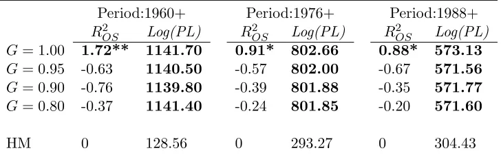
Table 3 presents the first set of core statistical results from our empirical analysis. The

overall story is clear: in terms of out-of-sample R2

, Clark and West (2007) test and log

predictive likelihood, DMMA outperforms HM for all subsample periods. Moreover, DMMA

has better results than other model combination methods including equal weights, BMA,

DMA in terms of point forecast accuracy.

We first examine Dynamic Mixture Model Averaging’s performances in greater detail

compared to the no-predictability benchmark in Table 3. DMMA takes all sources of model

uncertainties into account, allowing for different choices of predictors, varying degrees of

coef-ficient and forecasting models adaptivity. We find that DMMA significantly and consistently

outperforms HM, withR2

OS larger than zero and substantially larger log likelihoods than HM

across three different sample periods. The conclusion that DMMA has statistically lower

forecast errors than HM is confirmed by the CW test. This test rejects the null hypothesis

that the MSFE of HM is less than or equal to that of predictive model for all time periods. It

is worth noting that DMMA’s out-of-sample statistical performances slightly worsen during

period 1976+ and period 1988+, which is consistent with the finding that prediction accuracy

for forecasting excess stock returns may be driven by oil price shock in 1973-1975 and the

stock price crash in 1987 (Campbell and Thompson, 2008; Dangl and Halling, 2012; Joscha

and Sch¨ussler, 2014). However, DMMA still outperforms HM for sample periods 1976+ and

1988+, signalling that our framework is robust to many sample periods.

Next, we study the models that are nested by in DMMA and examine what features lead

to forecasting improvements. In particular, we present the results for equal weighted models,

Bayesian Model Averaging (BMA), and Dynamic Model Averaging (DMA) we built on, in

Panel B, C and D of Table 3 respectively. Looking at the results for equal weights (EW) in

Panel B, we find that the simple combination method, has reasonable performances. It is not

a surprise as a model with equal weights is a tough benchmark in the forecasting combination

literature (Rapach et al., 2010; Huang and Lee, 2010; Geweke and Amisano, 2012). We further

study how time-varying coefficient influences the results. R2

Table 3: Statistical Evaluation

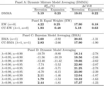
Panel A: Dynamic Mixture Model Averaging (DMMA)

Period:1960+ Period:1976+ Period:1988+

R2

OS(%) Log(PL) R2OS(%) Log(PL) R2OS(%) Log(PL)

DMMA 1.72** 1141.70 0.91* 802.66 0.88* 573.13

Panel B: Equal Weights (EW)

EW (α=0) 1.44** 1142.80 0.88* 803.05 0.67 573.31

CC-EW (λ=1,α=0) 0.92*** 1141.00 0.75** 802.78 0.62* 573.52

Panel C: Bayesian Model Averaging (BMA)

BMA (α=1) -1.26* 1133.30 -2.23 795.27 -0.15 571.08

CC-BMA (λ=1,α=1) -1.01* 1128.20 -2.35 793.53 -0.24 571.12

Panel D: Dynamic Model Averaging (DMA)

λ=0.90,α=0.90 -10.07 1092.70 -8.83 768.47 -10.34 547.14

λ=0.95,α=0.90 -10.60 1091.10 -9.41 767.47 -11.15 546.34

λ=0.99,α=0.90 -11.71 1091.00 -10.00 768.31 -11.48 547.33

λ=0.90,α=0.95 -6.18 1115.40 -5.67 784.89 -6.92 559.32

λ=0.95,α=0.95 -6.52 1114.10 -6.12 784.14 -7.57 558.79

λ=0.99,α=0.95 -6.32 1113.40 -5.89 784.28 -6.94 559.29

λ=0.90,α=0.99 -0.39 1136.50 -1.03 798.44 -1.23 569.43

λ=0.95,α=0.99 -0.53 1135.60 -1.16 798.11 -1.46 569.17

λ=0.99,α=0.99 -0.54 1133.80 -1.13 797.59 -1.47 569.04

HM 0 128.56 0 293.27 0 304.43

Notes: Statistical predictability for different models using out-of-sampleR2

(R2

OS(%)), Clark and West

equal model weights (CC-EW) deteriorates compared to time-varying coefficient with equal

weights (EW), confirming the finding in the literature that parameter instability matters for

return predictability.

Turing to Table 3 Panel C, we investigate Bayesian Model Averaging (BMA).

Interest-ingly, we find BMA cannot outperform HM for our dataset, with negative R2

OS. BMA is a

commonly used technique to tackle model uncertainty and to combine models together

ac-cording to their posterior probabilities (Avramov, 2002; Cremers, 2002; Dangl and Halling,

2012; Turner, 2015). However, the biggest problem of equal weights and BMA, as

acknowl-edged by Geweke and Amisano (2012), is that “they both condition on one of the models

under consideration being true.” Moreover, equal weights and BMA procedures assume their

method is appropriate across the whole sample period, which seems inappropriate especially

for the sporadically volatile stock market. DMMA, however, detects the locally

appropri-ate time-variation in coefficient and in forecasting model at each time. Therefore, it is not

surprising to find that DMMA improves upon models with equal weights (EW) and

mod-els with BMA with regard to R2

OS. These results suggest that allowing different degrees of

time-variation in forecasting model is important for improving forecast accuracy, as it flexibly

accommodates accommodating changes in data.

Last but not least, we employ possible specifications of Dynamic Model Averaging (DMA)

in Panel D of Table 3, in which we assume that coefficients and forecasting models change in

the same fashion over time. All DMAs do not forecast as well as HM and none of them have

positiveR2

OS andpvalues less than 10% for CW test. Moreover, data prefers gradual changes

in forecasting models, as the DMAs with α = 0.9 is much worse than the ones with α =

0.99, indicating the importance of choosing the exact time-variation in forecasting models.

In contrast, DMMA, the method based on DMA, has superior out-of-sample improvement

compared to DMA. This further confirms that even if we take time-varying coefficients and

forecasting models into account, predictability can still disappear if we ignore the importance

of evolving degrees of coefficients and models adaptivity.

All in all, DMMA substantially outperforms HM, equal weights, time-varying coefficients

with BMA as well as DMA across different subsample periods. By detecting locally

with misspecified models and quickly adapt the dynamics in the data generating process.10

Consequently, DMMA improves upon all the nested models in terms of out-of-sampleR2

.

4.1.2 Economic evaluation

In the previous section we confirm that large out-of-sample R2

OS can be obtained using

DMMA to predict stock returns, but is this meaningful for investors and traders?

Campbell and Thompson (2008) propose that if we can observe the predictors, the

per-centage increase for the expected return is :

R2

OS

1−R2

OS

1 +SR 2

SR2

(10)

where SR2

is the square of the Sharpe ratio. Equation (10) is larger than R2

OS/SR

2

, and

converges toR2

OS/SR

2

ifR2

OS and SR

2

are both small.

In light of this, the appropriate way to evaluate R2

OS is to calculate R

2

OS/SR

2

. If the

ratio is larger than 1, indicating that R2

OS is larger than SR

2

, investors can obtain higher

portfolio return by using the results in the predictive model. For instance, from Table 3

and 4 period 1960+ for DMMA model, we know R2

OS = 1.72% and SR

2 _{= 4.9%. A}

mean-variance investor thus can use DMMA to find out the optimal portfolio returns and increase

his average monthly portfolio returns substantially by 1.72%/4.9% = 35.1%.

Note that investors need to take risks to get the high portfolio return mentioned above.

To exclude risk especially for a mean-variance risk-averse investor who allocates his wealth

between equities and risk-free assets using forecasting results from our variance models, we

report certainty equivalent return (CER). The expected utility for the mean-variance investor

is:

U(Rp) =E(Rp)−

1

2γV ar(Rp) (11)

whereRpis the investors’ portfolio return,E(Rp) is the expected value of the return,V ar(Rp)

is the variance of the return and γ = 3.11

At the end oft, the investor optimally allocates a

10

Raftery et al. (2010) show that DMA rapidly accommodates changes in coefficients and changes in the entire forecasting models, by employing a simulation study. DMMA offers greater flexibility than DMA, and is capable to detect changes in the stock market.

11

portfolio weight in the risky asset

wt=

1 γ

ˆ rt+1

ˆ σ2

t+1

where ˆrt+1 is the forecast of excess stock return and ˆσ2_t+1 is the forecast of its variance.

Following Campbell and Thompson (2008) and Neely et al. (2014), we limit the percentage

invested in equities to be between 0% and 150% and assume that a five-year moving window

of past returns is used to estimate the variance forecasts.

The CER for the portfolio is

CERp = ˆµp−

1 2γσˆ

2

p (12)

where ˆµp and ˆσ2p are the mean and variance for the investor’s entire portfolio over the sample

period. Monthly CER are annualized by multiplying by 1200. Moreover, we consider the

effect of transaction costs in CER following Balduzzi and Lynch (1999) and Neely et al. (2014),

where the costs are measured using the percentage change of wealth traded each month and

assuming a proportional transactions cost equal to 50 basis points per transaction.

Table 4 shows certainty equivalent return (CER) and Sharp Ratio (SR) for different

models over different sample periods. The conclusion that DMMA has superior forecasts

than HM is confirmed and strengthened using this economic criteria. In particular, DMMA

hasCERat most 741 basis points and itsSR is larger than HM’s across all sample periods.

Compared with other predictive models, DMMA has good economic performance, and in

no case much worse than the best alternatives. A model with equal weights and Dynamic

Model Averaging (DMA) perform occasionally better than DMMA. Although DMMA

con-sistently has the best point forecast accuracy, there is slight disagreement between statistical

evaluation and economic evaluation. This is in consonance with the finding of Cenesizoglu

and Timmermann (2012) who suggest that there is a weak link between point forecast

accu-racy (e.g. out-of-sampleR2_{) and economic value. Interestingly, imposing constant coefficient}

restriction negatively affect model’s out-of-sample performance, indicating the importance of

Table 4: Economic Evaluation

Panel A: Dynamic Mixture Model Averaging (DMMA)

Period:1960+ Period:1976+ Period:1988+

CER SR CER SR CER SR

DMMA 5.15 0.08 6.24 0.10 7.41 0.15

Panel B: Equal Weights (EW)

EW (α=0) 5.44 0.09 6.34 0.11 7.26 0.14

CC-EW (λ=1,α=0) 4.15 0.07 5.54 0.10 7.09 0.14

Panel C: Bayesian Model Averaging (BMA)

BMA (α=1) 5.04 0.07 5.56 0.09 6.30 0.13

CC-BMA (λ=1,α=1) 2.49 0.03 4.13 0.07 5.74 0.12

Panel D: Dynamic Model Averaging (DMA)

λ=0.90,α=0.90 3.27 0.04 4.90 0.08 7.04 0.14

λ=0.95,α=0.90 3.39 0.04 4.48 0.07 6.62 0.13

λ=0.99,α=0.90 3.23 0.04 4.53 0.07 6.52 0.13

λ=0.90,α=0.95 4.12 0.05 5.05 0.08 7.01 0.14

λ=0.95,α=0.95 4.23 0.06 5.55 0.09 7.53 0.15

λ=0.99,α=0.95 4.89 0.07 5.85 0.09 7.56 0.15

λ=0.90,α=0.99 4.90 0.07 4.97 0.08 6.00 0.12

λ=0.95,α=0.99 4.72 0.07 4.81 0.08 6.05 0.12

λ=0.99,α=0.99 4.92 0.07 6.22 0.10 6.50 0.13

HM 3.39 0.07 3.93 0.08 5.25 0.12

4.2 Sources of Prediction Uncertainty

Our study is innovative since our DMMA approach can outperform the historical mean

statistically and economically, but also because we delineate forecast errors beyond the

stan-dard approach. This means that the relative importance for predictors, time-varying

coeffi-cients, and the individual model weights can be tracked over time. In this framework, the

prediction variance of the excess stock return can be decomposed. By doing so, we

under-stand our model’s underlying features and the source of forecasting power. This constitutes

one of the critical contributions of this paper.

We begin with the decomposition with regard to different degrees of time-variation in

modelsαz, based on the Law of Total Variance, prediction variance can be written as:

V ar(rt) =Eαz(V ar(rt|αz)) +V arαz(E(rt|αz)) (13)

whereEαz andV arαz are the expectation and prediction variance with regard toαz. We can

further decompose the termV ar(rt|αz) in equation (13) with respect to different degrees of

time-variation in coefficientsλj into:

V ar(rt|αz) =Eλj(V ar(rt|λj, αz)) +V arλj(E(rt|λj, αz)) (14)

Similarly,V ar(rt|λj, αz) in equation (14) can be written conditional on different choices of

predictorski:

Finally, substitute equation (15) and (14) into (13), we obtain:

V ar(rt) =Eki,λj,αz[V ar(rt|ki, λj, αz)] +Eλj,αz{V arki[E(rt|ki, λj, αz)]}

+Eαz{V arλj[E(rt|λj, αz)]}+V arαz[E(rt|αz)]

=X

z

{X

j

[(Ht|ki, λj, αz, Dt])P(ki |λj, αz, Dt)]P(λj |αz, Dt)}P(αz |Dt)

+X

z

{X

j

[(XtΣt+1|tX

′

t|ki, λj, αz, Dt)P(ki |λj, αz, Dt)]P(λj |αz, Dt)}P(αz |Dt)

+X

z

{X

j

[(ˆrj,z_t+1,i−rˆ j,z t+1)

2

P(ki |λj, αz, Dt)]P(λj |αz, Dt)}P(αz |Dt)

+X

z

[X

j

(ˆrj,z_t+1−rˆ

z t+1)

2

P(λj |αz, Dt)]P(αz |Dt)

+X

z

(ˆrz

t+1−rˆt+1)2P(αz |Dt)

(16)

Hence, equation (16) sheds light on the sources of uncertainty of return prediction.

In-tuitively, the first term captures the expected variance of the innovation term in the

mea-surement equation, conditional on the choices of predictors ki, degree of time-variation in

coefficients λj and model αz. We call it observational variance. The second term indicates

the expected variance of errors in coefficients, which can be classified as estimation

uncer-tainty in coefficients. Whereas, the remaining components of equation (16) are referred to as

model uncertainty. In particular, the third term characterizes model uncertainty with regard

to predictor selection. The forth term measures model uncertainty in terms of degree of

time-variation in the coefficients. Finally, the fifth term states model uncertainty regarding

the degree of time-variation in forecasting models. Dangl and Halling (2012) consider the

first four sources of forecast errors. To the best of our knowledge, ours is the first paper in the

return predictability literature that investigates model uncertainty with respect to different

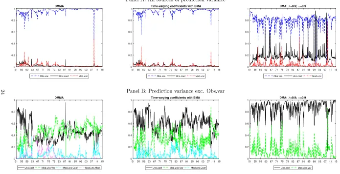
Figure 1: Sources of Prediction Variance for DMMA, BMA and DMA

Panel A: All sources of prediction variance

51 55 59 63 67 71 75 79 83 87 91 95 99 03 07 11 15 0 0.2 0.4 0.6 0.8 1 DMMA

Obs.var. Unc.coef Mod.unc

51 55 59 63 67 71 75 79 83 87 91 95 99 03 07 11 15 0

0.2 0.4 0.6 0.8

1 Time-varying coefficients with BMA

Obs.var. Unc.coef Mod.unc

51 55 59 63 67 71 75 79 83 87 91 95 99 03 07 11 15 0 0.2 0.4 0.6 0.8 1 DMA:

λ=0.9; α=0.9

Obs.var. Unc.coef Mod.unc

Panel B: Prediction variance exc. Obs.var

51 55 59 63 67 71 75 79 83 87 91 95 99 03 07 11 15 0 0.2 0.4 0.6 0.8 1 DMMA

Unc.coef Mod.unc.Var Mod.unc.Coef Mod.unc.Mod.

51 55 59 63 67 71 75 79 83 87 91 95 99 03 07 11 15 0

0.2 0.4 0.6 0.8

1 Time-varying coefficients with BMA

Unc.coef Mod.unc.Var Mod.unc.Coef

51 55 59 63 67 71 75 79 83 87 91 95 99 03 07 11 15 0 0.2 0.4 0.6 0.8 1

DMA: λ=0.9; α=0.9

Unc.coef Mod.unc.Var

Notes: Decomposition of the prediction variance for DMMA, possible degrees of time-variation in coefficients with BMA and DMA (takeλ= 0.9, α= 0.9 as an example). Panel A of the Figure plots the relative weights of observational variance (Obs.var.), expected variance from errors in the estimation of coefficients (Unc.coef.) and variance caused by the model uncertainty (Mod.unc.). Panel B excludes observational variance and investigates expected variance from errors in the estimation of coefficients (Unc.coef.), variance caused by the uncertainty regarding the variable selection (Mod.unc.Var), variance caused by the uncertainty regarding different degrees of time-variation in coefficients (Mod.unc.Coef) and in forecasting models (Mod.unc.Mod). Particularly, in Panel B, for time-varying

Figure 1 depicts different sources of prediction variance for three approaches: (i) DMMA,

(ii) possible degrees of time-variation in coefficients with BMA (α= 1) and (iii) DMA model

(takeλ= 0.9, α= 0.9 as an example).12

Panel A of the Figure shows the relative weights of

observational variance (Obs.var.), uncertainty about estimating coefficients (Unc.coef.) and

model uncertainty (Mod.unc.).13

For all three approaches observational variance dominates.

Dangl and Halling (2012), claim that this is conventional for stock return prediction

be-cause random fluctuations are expected to be-cause considerable volatility, especially for the one

month forecast horizons we consider. Specifically, for DMMA and BMA, estimation risk and

model uncertainty are small except for the initial data-points of the out-of-sample predictive

process14

and the peak of model uncertainty during the financial crisis in 2008. Whereas, for

DMA, estimation uncertainty accounts for around 20% of the total prediction variance and

model uncertainty is nonnegligible.

There are also notable differences between our three models. With respect to estimation

uncertainty and variance caused by predictor selection in Panel B of Figure 1, there are

notable differences among DMMA, BMA and DMA. Importantly, for DMMA, uncertainty

regrading coefficient estimation accounts for the largest proportion in the initial data points,

however, it is of less importance after 1965. In the meantime, uncertainty with regard to

predictor selection becomes crucial. Whereas, when we fix time-variation in the forecasting

model using BMA, estimation uncertainty in coefficients dominates the remaining variance for

most periods, only with occasional switches to model uncertainty with respect to predictor

selection. If the coefficient and forecasting models change in the same fashion over time

(DMA), estimation risk is prominent at the start of the sample. These first imply that

observational uncertainty, estimation uncertainty and uncertainty with respect to predictor

selection are the top three sources of prediction variance that hinder forecasting performance

for different models. Second, DMMA has the smallest estimation error among different

12

We considerλ= 0.9, α= 0.9 because they represent extremely rapidly changing coefficient and forecasting models, which seems unreasonable in the stock market. Our aim is to demonstrate different sources of uncertainty when we choose inappropriate parameters.

13

We present absolute values of different variances in the online appendix. DMA has the largest prediction variance. DMMA, in contrast, has the smallest variance.

14

alternatives, whereas, when we select an inappropriate degree of time-variation in coefficients

and in forecasting models, the estimation risk can be large.

Besides, turning to the rest of the model uncertainty in DMMA, we uncover that

un-certainty regarding different choices of time-variation is negligible after the initial 30 years,

implying that learning the dynamics in the time-varying forecasting models can take some

time. Uncertainty with regard to different choices of time-variation in coefficients, however,

is low except for the fluctuations around recessions (e.g., the post-Korean War recession

between 1953-1954, the oil shock around 1973 and the financial crisis from 2007).

Importantly, uncertainty with respect to predictor selection cannot be neglected and it

seems to be critical in leading forecasting improvements. As we will demonstrate in section

4.4 when we study the role of different predictors, all the predictors tend to be important

in forecasting equity premium. This implies that the ensemble of features of DMMA is

necessary, including combining multiple predictors, allowing varying degrees of coefficients

adaptivity and different degrees of time-variation in forecasting models.

In spite of the fact that estimation uncertainty in coefficients is one of the key factors

obstructing forecasting performance, our fully flexible DMMA model outperforms

alterna-tives because it makes use of all the information in the dataset. In other words, our model

effectively adapts the pattern in the unstable stock market by embedding the precise level

of time-variation in coefficients and forecasting models, thus, the variances due to

uncer-tainty about the choice of degree of time-variation in coefficients and forecasting models are

small. When comparing the differences of variance decomposition between BMA and DMA,

one possible explanation for DMMA’s superior out-of-sample performance is that considering

possible range of time-variation in coefficients increase coefficient variability, thus, offset the

loss in forecast accuracy caused by the second largest source of prediction variance:

coeffi-cients estimation uncertainty. Moreover, by allowing for different degrees of time-variation

in forecasting models, DMMA enhances model adaptability and quickly detects locally

ap-propriate models, therefore, improves upon time-varying coefficients with BMA and further

4.3 Link predictability to the business cycle

Previously, we provided evidence of economic and statistical predictability of our DMMA

model relative to others over different sample periods. We also analyze what leads to

forecast-ing improvements by decomposforecast-ing variance. In this section, we link DMMA’s predictability

to the business cycle.

Theoretically, excess stock returns predictability is closely related to the business

cy-cle(Fama and French, 1989; Campbell and Cochrane, 1995; Cochrane, 1999, 2005; Rapach

et al., 2010; Dangl and Halling, 2012). In general, investors are more risk-averse during

re-cessions, who, in turn, ask for much higher excess stock returns for risk compensation. As

a consequence, the equity premium tends to decrease during expansions and increase

dur-ing recessions. Moreover, local maxima of the equity risk premia often appears to be near

business cycles troughs, whereas, local minima occurs near business cycles peaks (Fama and

French, 1989; Campbell and Cochrane, 1995; Cochrane, 1999). In this framework, DMMA’s

predictability would rise if it could capture the business cycle (Rapach et al., 2010; Henkel

et al., 2011; Dangl and Halling, 2012).

Rapach et al. (2010) systematically and empirically study the link between prediction

improvements and business cycle. Similarly, they predict equity premium by combining

in-dividual predictive regression models together and find that the combination method has

superior out-of-sample prediction of excess stock returns which, in turn, better links to the

business cycle when comparing to individual forecasts and the historical mean model.

Ra-pach et al. (2010) argue that the reason why the historical mean model cannot capture

business-cycle fluctuations is because it always produces a very smooth prediction, therefore,

fails to incorporate macroeconomic information. With respect to the individual predictive

regressions, they may contain false signals and exhibit implausible fluctuations.

We use NBER recessions and expansions data to identify how close the predictability of

the DMMA model is linked to the business cycle. Table 5 reports two statistics: out-of-sample

R2

(R2

OS) and CER gains (∆CER) relative to the no-predictability benchmark during

re-cessions and expansions over different sample periods for various predictive models. When

Table 5: Business Cycle Analysis

Panel A: Dynamic Mixture Model Averaging (DMMA)

R2

OS(%) ∆CER

Recession Expansion Recession Expansion

DMMA 5.19 0.23 19.01 0.22

Panel B: Equal Weights (EW)

EW (α=0) 4.22 0.25 17.90 0.18

CC-EW (λ=1,α=0) 1.93 0.48 5.18 0.63

Panel C: Bayesian Model Averaging (BMA)

BMA (α=1) 2.60 -2.92 20.65 -1.31

CC-BMA (λ=1,α=1) 2.83 -2.66 17.90 -1.90

Panel D: Dynamic Model Averaging

λ=0.90,α=0.90 -10.70 -9.80 18.14 -2.78

λ=0.95,α=0.90 -11.56 -10.19 18.56 -2.88

λ=0.99,α=0.90 -12.40 -11.42 19.66 -2.62

λ=0.90,α=0.95 -7.74 -5.52 22.80 -2.87

λ=0.95,α=0.95 -8.40 -5.71 21.25 -2.78

λ=0.99,α=0.95 -6.70 -6.15 23.00 -2.39

λ=0.90,α=0.99 2.11 -1.46 12.04 -1.87

λ=0.95,α=0.99 1.79 -1.53 12.32 -1.63

λ=0.99,α=0.99 2.44 -1.81 17.37 -1.23

Notes: Business cycle analysis using out-of-sample R2

(R2

OS(%)) and certainty equivalent return gain

recessions than expansions. In terms of economic evaluation, DMMA shows its unique power

to generate considerable returns especially in recessions, withCER gains during recessions

approximately 41 times larger than that during expansions. The fact that predictability will

rise during recessions is in line with the empirical evidence provided by Rapach et al. (2010),

Henkel et al. (2011) and Dangl and Halling (2012). Researchers argue that this is because

HM model overestimates the equity premium, therefore, suffers from huge losses particularly

in recessions. Interestingly, DMMA also has positive out-of-sampleR2 _{and CER gains}

dur-ing expansions, which further confirms the strong predictability of DMMA. This result is

consistent with the findings of Dangl and Halling (2012), who claim there is predictability

during expansions using their predictors and econometric method.

Comparing with other models, DMMA has superior predictive power especially during

recessions. Whereas, constant coefficients with equal weights (CC-EW) perform well during

expansions, with its out-of-sample R2

and CER gains both slightly larger than DMMA’s.

We cannot find predictability for DMA and BMA models during expansions, confirming the

conclusion in Section 4.4.2 that data is mainly in favor of models with equal weights and

constant coefficients. However, the biggest difference between DMMA and CC-EW is that

DMMA detects dynamics in the stock market by embedding the exact degree of time-variation

in coefficients and in forecasting models at each point in time. In contrast, CC-EW is static

and over-optimistic, thus will be unable to adapt to changes during recessions. This leads to

DMMA’s improvements upon CC-EW especially during downturns.

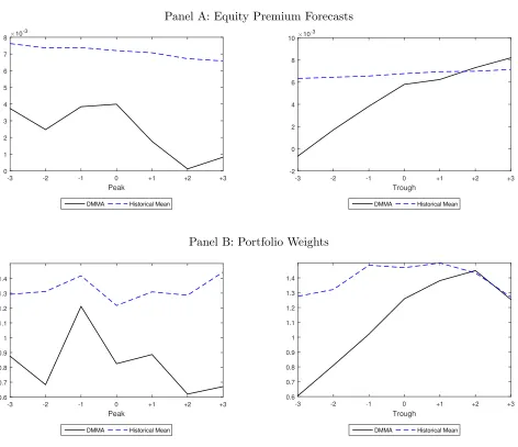
Next, we closely look at the equity premium predictions and portfolio weights of risky

asset around turning points of the business cycle. Figure 2 Panel A shows the predicted

equity premiums around peaks and troughs. Predictions from DMMA fit the theoretical

pattern acknowledged by Cochrane (1999, 2005): the predicted equity premium increases

at the end of recession, signalling greater risk-aversion during recessions. In addition, local

minima seems to be around the peak. In contrast, investors who believe in the HM model are

over optimistic and predictions from HM are too smooth to capture the fluctuations around

business-cycle turning points.

We also uncover that a mean-variance optimizer who relies on DMMA appears to perfectly

Figure 2: Equity Premium Forecasts and Portfolio Weights Around Peaks and Troughs

Panel A: Equity Premium Forecasts

Peak

-3 -2 -1 0 +1 +2 +3

×10-3

0 1 2 3 4 5 6 7 8

DMMA Historical Mean

Trough

-3 -2 -1 0 +1 +2 +3

×10-3

-2 0 2 4 6 8 10

DMMA Historical Mean

Panel B: Portfolio Weights

Peak

-3 -2 -1 0 +1 +2 +3

0.6 0.7 0.8 0.9 1 1.1 1.2 1.3 1.4

DMMA Historical Mean

Trough

-3 -2 -1 0 +1 +2 +3

0.6 0.7 0.8 0.9 1 1.1 1.2 1.3 1.4

DMMA Historical Mean

N otes: Panel A demonstrate the predicted equity premium using DMMA and historical mean. Panel B

DMMA pull out of the stock market rapidly when the recession starts, and gradually increase

equity holdings towards the end of recession. Whereas, HM gives investors false signals,

making them fail to withdraw money from the equity market at the beginning of a recession.

We conclude that the predictions from the historical mean cannot capture the abrupt

changes in the stock market and are less economically meaningful. The agreement between

DMMA’s predictions and asset price theory suggested by Cochrane (1999, 2005) provide more

economic insights of equity premium predictability.

4.4 Model characteristics

4.4.1 Which predictor is important?

Given that we have 12 macroeconomic predictors and 14 technical predictors for excess

stock return, it would be interesting to see which one is the most important and how a

predic-tor evolves over time. We measure this by presenting the posterior inclusion probability for

each predictor at each time, which can be obtained using DMMA. Following the econometric

framework mentioned above, we know that our predictive models are constructed in a way

that only a single predictor is included in each model, thus, the posterior inclusion

probabil-ity for each predictor can be treated as the posterior model probabilities. Therefore, if the

posterior model probability for a model or the posterior inclusion probability for a variable

is high, that model is likely to be the true model and that variable may play an important

role in predicting excess stock returns.

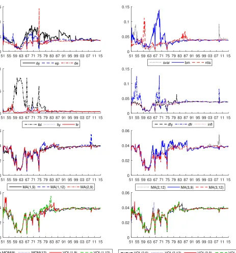
Figure 3 presents the time-varying posterior probabilities for the 26 predictors. From the

initial data points until 1975, the shifts between different predictors are occasional and mostly

between macroeconomic predictors: treasury bill rate (tbl), default yield spread (dfr),

book-to-market ratio (bm), dividend yield (dy) and net equity expansion (ntis). Especially, treasury

bill rate (tbl) is highly informative for stock prediction during 1957 to 1967 and 1973 to 1975.

After 1975, however, technical indicators become essential and have the similar predictive

power as macroeconomic indicators, with inclusion probabilities for different predictors all

around 0.04, only with several spikes around the financial crisis in 2008 (e.g., see stock variance

Figure 3: Time-Varying Inclusion Probabilities for Different Predictors

51 55 59 63 67 71 75 79 83 87 91 95 99 03 07 11 15 0

0.05 0.1 0.15

dy ep de

51 55 59 63 67 71 75 79 83 87 91 95 99 03 07 11 15 0

0.05 0.1 0.15

svar bm ntis

51 55 59 63 67 71 75 79 83 87 91 95 99 03 07 11 15 0

0.5 1

tbl lty ltr

51 55 59 63 67 71 75 79 83 87 91 95 99 03 07 11 15 0

0.05 0.1 0.15

dfy dfr infl

51 55 59 63 67 71 75 79 83 87 91 95 99 03 07 11 15 0

0.02 0.04 0.06

MA(1,9) MA(1,12) MA(2,9)

51 55 59 63 67 71 75 79 83 87 91 95 99 03 07 11 15 0

0.02 0.04 0.06

MA(2,12) MA(3,9) MA(3,12)

51 55 59 63 67 71 75 79 83 87 91 95 99 03 07 11 15 0

0.02 0.04 0.06

MOM(9) MOM(12) VOL(1,9) VOL(1,12)

51 55 59 63 67 71 75 79 83 87 91 95 99 03 07 11 15 0

0.02 0.04 0.06

VOL(2,9) VOL(2,12) VOL(3,9) VOL(3,12)

view that DMMA attaches approximately equal weights to each predictor from 1975 to the end

of the sample period, and is consistent with the finding acknowledged by Neely et al. (2014)

that macroeconomic predictors and technical predictors have complementary information.

Moreover, we find that none of the predictor’s posterior probabilities consistently exceeds the

prior of 1/26 over time. This confirms the result in Section 4.2 that there is nonnegligible

uncertainty about the best predictor. Under this condition, DMMA automatically detects

the best predictor while attaching low posterior weight to the ones that perform poorly over

time.

4.4.2 Analysis of different degrees of time-variation in coefficients and in

fore-casting models

The preceding results show that using DMMA, we can adapt the pattern in data by

embedding the exact level of time-variation in coefficients and forecasting models. Next we

demonstrate the empirical evidence for that.

We closely look at posterior probabilities for possible degrees of time-variation in

coeffi-cients for DMMA in Figure 4. In general, models with constant coefficoeffi-cients and gradually

changing coefficients are informative about the movements of equity premium. In contrast,

models with sudden changes in coefficients lose data support at the beginning of the sample.

Moreover, observations around the oil shock in 1975 and the financial crisis in 2008 enhance

the occasional evidence in favor of time-varying coefficients.

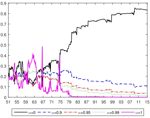
Figure 5 presents the posterior probabilities of different degrees of time-variation in

fore-casting models. Equal weighted (α = 0) models dominate other situations such as BMA

(α= 1), abruptly changing predictive density combination and a gradually changing

predic-tive density combination after a period of adjustment until 1975. Whereas, BMA is favored

by the data at the beginning of out-of-sample period, with its inclusion probability larger

than prior 0.2 during 1960 to 1965 and spikes in 1967 and 1975. The dominance of a certain

value of α for a prolonged period is reflected in the negligible uncertainty with respect to

the degree of time-variation in forecasting models. Moreover, high inclusion probability for

equal weighted models from 1975 is in line with the finding in Section 4.4.1: DMMA attaches

Figure 4: Posterior Probabilities of Degrees of Time-variation in Coefficients (λ)

51 55 59 63 67 71 75 79 83 87 91 95 99 03 07 11 15 0

0.2 0.4 0.6 0.8 1

λ=0.9 λ=0.95 λ=0.99 λ=1

Notes: Posterior probabilities of models with a specific degree of time-variation of coefficients (λ) for DMMA. Particularly,λ∈_[0.90,0.95,0.99,1].

Figure 5: Posterior Probabilities of Degrees of Time-variation in Forecasting Models (α)

51 55 59 63 67 71 75 79 83 87 91 95 99 03 07 11 15 0

0.1 0.2 0.3 0.4 0.5 0.6 0.7 0.8 0.9

α=0 α=0.9 α=0.95 α=0.99 α=1

5

Conclusion

The literature on stock return forecasting suggests that the out-of-sample predictability

is erratic (Cooper and Gulen, 2006; Andrew and Geert, 2007; Campbell and Thompson,

2008; Welch and Goyal, 2008; Joscha and Sch¨ussler, 2014; Turner, 2015). Even though

occasionally predictive power is found, it seems to be specific to some predictors in some

sample periods, signalling the presence of model instability and uncertainty. Although there

have been several attempts to take account of them, there is not a consensus on the exact

degree of time-variation in coefficients and the method to combine all the individual models

using different predictors. In this paper, we solve these problems by constructing Dynamic

Mixture Model Averaging (DMMA), which incorporates possible degrees of time-variation

in coefficients and in forecasting models, to detect locally appropriate models. Especially,

instead of imposing ex-ante that coefficients and forecasting models vary in the same fashion

over time, we encompass moderate to abrupt changes and even no-change in coefficients and

forecasting models.

What we uncover is that DMMA model generate more accurate forecasts compared to

the historical mean (HM) benchmark across different sample periods. These statistical gains

also lead to superior economic profits for a mean-variance investor. Most importantly, in

terms of point accuracy, DMMA dominates its nested model combination method including

Bayesian Model Averaging (BMA), Dynamic Model Averaging (DMA) and equal weighted

models. This implies the importance of accommodating different degrees of time-variation in

coefficients and multiple degrees of time-varying forecasting model adaptability.

We further pin down the origins of forecasting improvements by tracking different sources

of uncertainty in the predictive regressions. Besides the observational variance, uncertainty

regarding the errors from estimating the coefficients and model uncertainty with respect to

predictor selection are the key factors hindering forecast accuracy. In contrast, uncertainty

about the degree of time-variation in coefficients is small and uncertainty regarding the degree

of time-variation in forecasting models is only notable at the initial data points. Essentially,

DMMA successfully reduces uncertainty regarding estimation error compared to other