Improving Lexical Embeddings with Semantic Knowledge

Improving Lexical Embeddings with Semantic Knowledge

Machine Translation Lab Harbin Institute of Technology

Harbin, China gflfof@gmail.com

Mark Dredze

Human Language Technology Center of Excellence Center for Language and Speech Processing

Johns Hopkins University Baltimore, MD 21218 mdredze@cs.jhu.edu

Abstract

Word embeddings learned on unlabeled data are a popular tool in semantics, but may not capture the desired semantics. We propose a new learning objective that in-corporates both a neural language model objective (Mikolov et al., 2013) and prior knowledge from semantic resources to learn improved lexical semantic dings. We demonstrate that our embed-dings improve over those learned solely on raw text in three settings: language mod-eling, measuring semantic similarity, and predicting human judgements.

1 Introduction

Word embeddings are popular representations for syntax (Turian et al., 2010; Collobert and We-ston, 2008; Mnih and Hinton, 2007), semantics (Huang et al., 2012; Socher et al., 2013), morphol-ogy (Luong et al., 2013) and other areas. A long line of embeddings work, such as LSA and ran-domized embeddings (Ravichandran et al., 2005; Van Durme and Lall, 2010), has recently turned to neural language models (Bengio et al., 2006; Collobert and Weston, 2008; Turian et al., 2010). Unsupervised learning can take advantage of large corpora, which can produce impressive results.

However, the main drawback of unsupervised learning is that the learned embeddings may not be suited for the task of interest. Consider se-mantic embeddings, which may capture a notion of semantics that improves one semantic task but harms another. Controlling this behavior is chal-lenging with an unsupervised objective. However, rich prior knowledge exists for many tasks, and there are numerous such semantic resources.

We propose a new training objective for learn-ing word embeddlearn-ings that incorporates prior

∗

This work was done while the author was visiting JHU.

knowledge. Our model builds on word2vec (Mikolov et al., 2013), a neural network based language model that learns word embeddings by maximizing the probability of raw text. We extend the objective to include prior knowledge about synonyms from semantic resources; we consider both the Paraphrase Database (Ganitkevitch et al., 2013) and WordNet (Fellbaum, 1999), which an-notate semantic relatedness between words. The latter was also used in (Bordes et al., 2012) for training a network for predicting synset relation. The combined objective maximizes both the prob-ability of the raw corpus and encourages embed-dings to capture semantic relations from the re-sources. We demonstrate improvements in our embeddings on three tasks: language modeling, measuring word similarity, and predicting human judgements on word pairs.

2 Learning Embeddings

We present a general model for learning word em-beddings that incorporates prior knowledge avail-able for a domain. While in this work we con-sider semantics, our model could incorporate prior knowledge from many types of resources. We be-gin by reviewing the word2vec objective and then present augmentations of the objective for prior knowledge, including different training strategies.

2.1 Word2vec

Word2vec (Mikolov et al., 2013) is an algorithm for learning embeddings using a neural language model. Embeddings are represented by a set of latent (hidden) variables, and each word is rep-resented by a specific instantiation of these vari-ables. Training learns these representations for each wordwt(thetth word in a corpus of sizeT) so as to maximize the log likelihood of each token given its context: words within a window sizedc:

max_T1 XT

t=1

logp wt|wtt+c−c

, (1)

wherewt+c_t−c is the set of words in the window of sizeccentered atwt(wtexcluded).

Word2vec offers two choices for modeling of Eq. (1): a skip-gram model and a continuous bag-of-words model (cbow). The latter worked better in our experiments so we focus on it in our presen-tation. cbow definesp(wt|wt+ct−c)as:

expe0_wt>·P_{−c≤j≤c,j6=0}ewt+j

P wexp

e0

w>·P−c≤j≤c,j6=0ewt+j

, (2)

where ew and e0w represent the input and output embeddings respectively, i.e., the assignments to the latent variables for wordw. While some learn a single representation for each word (e0

w , ew), our results improved when we used a separate em-bedding for input and output in cbow.

2.2 Relation Constrained Model

Suppose we have a resource that indicates rela-tions between words. In the case of semantics, we could have a resource that encodes semantic similarity between words. Based on this resource, we learn embeddings that predict one word from another related word. We defineRas a set of rela-tions between two wordswandw0_{.Rcan contain}

typed relations (e.g., w is related to w0 _through

a specific type of semantic relation), and rela-tions can have associated scores indicating their strength. We assume a single relation type of uni-form strength, though it is straightforward to in-clude additional characteristics into the objective.

Define Rw to be the subset of relations in R which involve wordw. Our objective maximizes the (log) probability of all relations by summing over all wordsN in the vocabulary:

1

N N X

i=1 X

w∈R_wi

logp(w|wi), (3)

p(w|wi) = exp

e0

wTewi

/P_w¯expe0

¯ wTewi

takes a form similar to Eq. (2) but without the context: e and e0 _{are again the input and output}

embeddings. For our semantic relations e0

w and

eware symmetrical, so we use a single embedding. Embeddings are learned such that they are predic-tive of related words in the resource. We call this the Relation Constrained Model (RCM).

2.3 Joint Model

The cbow and RCM objectives use separate data for learning. While RCM learns embeddings

suited to specific tasks based on knowledge re-sources, cbow learns embeddings for words not in-cluded in the resource but appear in a corpus. We form a joint model through a linear combination of the two (weighted byC):

1

T T X

t=1

logp wt|wtt+c−c

+_NC XN

i=1 X

w∈R_wi

logp(w|wi)

Based on our initial experiments, RCM uses the output embeddings of cbow.

We learn embeddings using stochastic gradient ascent. Updates for the first term fore0 _andeare:

e0_w−αcbow σ(f(w))−I[w=wt]

· Xt+c

j=t−c ewj

ewj−αcbow

X

w

σ(f(w))−I_[w=wt]·e0

w,

where σ(x) = exp{x}/(1 + exp{x}), I_[x] is 1 whenxis true,f(w) =e0

w>Pt+cj=t−cewj. Second

term updates are: e0

w−αRCM

σ(f0_(w))−I

[w∈R_wi]

·e0

wi

e0_wi−αRCM

X

w

σ(f0(w))−I[w∈R_wi]

·e0_w,

where f0_{(w) = e}0

w>e0wi. We use two learning

rates:αcbowandαRCM. 2.4 Parameter Estimation

All three models (cbow, RCM and joint) use the same training scheme based on Mikolov et al. (2013). There are several choices to make in pa-rameter estimation; we present the best perform-ing choices used in our results.

We use noise contrastive estimation (NCE) (Mnih and Teh, 2012), which approximately max-imizes the log probability of the softmax objec-tive (Eq. 2). For each objecobjec-tive (cbow or RCM), we sample 15 words as negative samples for each training instance according to their frequencies in raw texts (i.e. training data of cbow). Supposew has frequencyu(w), then the probability of sam-plingwisp(w)∝u(w)3/4_.

We use distributed training, where shared em-beddings are updated by each thread based on training data within the thread, i.e., asynchronous stochastic gradient ascent. For the joint model, we assign threads to the cbow or RCM objective with a balance of 12:1(i.e.Cis approximately 1

for balancing the two objectives. We trained each cbow objective using a single pass over the data set (except for those in Section 4.1), which we empir-ically verified was sufficient to ensure stable per-formances on semantic tasks.

Model pre-training is critical in deep learning (Bengio et al., 2007; Erhan et al., 2010). We eval-uate two strategies: random initialization, and pre-training the embeddings. For pre-pre-training, we first learn using cbow with a random initialization. The resulting trained model is then used to initialize the RCM model. This enables the RCM model to benefit from the unlabeled data, but refine the em-beddings constrained by the given relations.

Finally, we consider a final model for training embeddings that uses a specific training regime. While the joint model balances between fitting the text and learning relations, modeling the text at the expense of the relations may negatively impact the final embeddings for tasks that use the embed-dings outside of the context of word2vec. There-fore, we use the embeddings from a trained joint model to pre-train an RCM model. We call this setting Joint→RCM.

3 Evaluation

For training cbow we use the New York Times (NYT) 1994-97 subset from Gigaword v5.0 (Parker et al., 2011). We select 1,000 paragraphs each for dev and test data from the December 2010 portion of the NYT. Sentences are tokenized using OpenNLP1_{, yielding 518,103,942 tokens for}

train-ing, 42,953 tokens for dev and 41,344 for test. We consider two resources for training the RCM term: the Paraphrase Database (PPDB) (Ganitkevitch et al., 2013) and WordNet (Fell-baum, 1999). For each semantic pair extracted from these resources, we add a relation to the RCM objective. Since we use both resources for evaluation, we divide each into train, dev and test. PPDB is an automatically extracted dataset con-taining tens of millions of paraphrase pairs, in-cluding words and phrases. We used the “lexi-cal” version of PPDB (no phrases) and filtered to include pairs that contained words found in the 200,000 most frequent words in the NYT corpus, which ensures each word in the relations had sup-port in the text corpus. Next, we removed dupli-cate pairs: if <A,B>occurred in PPDB, we re-moved relations of <B,A>. PPDB is organized

1_{https://opennlp.apache.org/}

PPDB Relations WordNet Relations

Train XL 115,041 Train 68,372

XXL 587,439 (not used in XXXL 2,647,105 this work)

Dev 1,582 Dev 1,500

Test 1,583 Test 1,500

Table 1: Sizes of semantic resources datasets.

into 6 parts, ranging from S (small) to XXXL. Division into these sets is based on an automat-ically derived accuracy metric. Since S contains the most accurate paraphrases, we used these for evaluation. We divided S into a dev set (1582 pairs) and test set (1583 pairs). Training was based on one of the other sets minus relations from S.

We created similar splits using WordNet, ex-tracting synonyms using the 100,000 most fre-quent NYT words. We divide the vocabulary into three sets: the most frequent 10,000 words, words with ranks between 10,001-30,000 and 30,001-100,000. We sample 500 words from each set to construct a dev and test set. For each word we sample one synonym to form a pair. The remain-ing words and their synonyms are used for train-ing. However we did not use the training data be-cause it is too small to affect the results. Table 1 summarizes the datasets.

4 Experiments

The goal of our experiments is to demonstrate the value of learning semantic embeddings with infor-mation from semantic resources. In each setting, we will compare the word2vec baseline embed-ding trained with cbow against RCM alone, the joint model and Joint→RCM. We consider three evaluation tasks: language modeling, measuring semantic similarity, and predicting human judge-ments on semantic relatedness. In all of our ex-periments, we conducted model development and tuned model parameters (C, αcbow, αRCM, PPDB

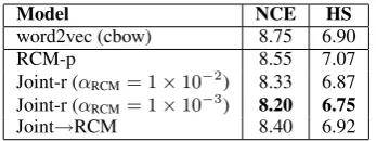
Model NCE HS word2vec (cbow) 8.75 6.90

RCM-p 8.55 7.07

Joint-r (αRCM= 1×10−2) 8.33 6.87

Joint-r (αRCM= 1×10−3) 8.20 6.75

Joint→RCM 8.40 6.92

Table 2: LM evaluation on held out NYT data.

We trained 200-dimensional embeddings and used output embeddings for measuring similarity. Dur-ing the trainDur-ing of cbow objectives we remove all words with frequencies less than 5, which is the default setting of word2vec.

4.1 Language Modeling

Word2vec is fundamentally a language model, which allows us to compute standard evaluation metrics on a held out dataset. After obtaining trained embeddings from any of our objectives, we use the embeddings in the word2vec model to measure perplexity of the test set. Measuring perplexity means computing the exact probability of each word, which requires summation over all words in the vocabulary in the denominator of the softmax. Therefore, we also trained the language models with hierarchical classification (Mikolov et al., 2013) strategy (HS). The averaged perplexi-ties are reported on the NYT test set.

While word2vec and joint are trained as lan-guage models, RCM is not. In fact, RCM does not even observe all the words that appear in the train-ing set, so it makes little sense to use the RCM em-beddings directly for language modeling. There-fore, in order to make fair comparison, for every set of trained embeddings, we fix them as input embedding for word2vec, then learn the remain-ing input embeddremain-ings (words not in the relations) and all the output embeddings using cbow. Since this involves running cbow on NYT data for 2 it-erations (one iteration for word2vec-training/pre-training/joint-modeling and the other for tuning the language model), we use Joint-r (random ini-tialization) for a fair comparison.

Table 2 shows the results for language mod-eling on test data. All of our proposed models improve over the baseline in terms of perplexity when NCE is used for training LMs. When HS is used, the perplexities are greatly improved. How-ever in this situation only the joint models improve the results; and Joint→RCM performs similar to the baseline, although it is not designed for lan-guage modeling. We include the optimal αRCM

in the table; while setαcbow = 0.025(the default

setting of word2vec). Even when our goal is to strictly model the raw text corpus, we obtain im-provements by injecting semantic information into the objective. RCM can effectively shift learning to obtain more informative embeddings.

4.2 Measuring Semantic Similarity

Our next task is to find semantically related words using the embeddings, evaluating on relations from PPDB and WordNet. For each of the word pairs in the evaluation set<A,B>, we use the co-sine distance between the embeddings to scoreA with a candidate wordB0_{. We use a large sample}

of candidate words (10k, 30k or 100k) and rank all candidate words for pairs whereB appears in the candidates. We then measure the rank of the cor-rectB to compute mean reciprocal rank (MRR). Our goal is to use word A to select word B as the closest matching word from the large set of candidates. Using this strategy, we evaluate the embeddings from all of our objectives and mea-sure which embedding most accurately selected the true correct word.

Table 3 shows MRR results for both PPDB and WordNet dev and test datasets for all models. All of our methods improve over the baselines in nearly every test set result. In nearly every case, Joint→RCM obtained the largest improvements. Clearly, our embeddings are much more effective at capturing semantic similarity.

4.3 Human Judgements

Our final evaluation is to predict human judge-ments of semantic relatedness. We have pairs of words from PPDB scored by annotators on a scale of 1 to 5 for quality of similarity. Our data are the judgements used by Ganitkevitch et al. (2013), which we filtered to include only those pairs for which we learned embeddings, yielding 868 pairs. We assign a score using the dot product between the output embeddings of each word in the pair, then order all 868 pairs according to this score. Using the human judgements, we compute the swapped pairs rate: the ratio between the number of swapped pairs and the number of all pairs. For pairpscoredypby the embeddings and judgedyˆp by an annotator, the swapped pair rate is:

P

p1,p2∈D_PI[(yp1 −yp2) (ˆyp2 −yˆp1)<0] p1,p2∈DI[yp1 6=yp2]

(4)

PPDB WordNet

Model _10k Dev_{30k 100k 10k} Test_{30k 100k 10k} Dev_{30k 100k 10k} Test_{30k 100k} word2vec (cbow) 49.68 39.26 29.15 49.31 42.53 30.28 10.24 8.64 5.14 10.04 7.90 4.97

word2vec (skip-gram) 48.70 37.14 26.20 - - - 8.61 8.10 4.62 - -

-RCM-r 55.03 42.52 26.05 - - - 13.33 9.05 5.29 - -

-RCM-p 61.79 53.83 40.95 65.42 55.82 41.20 15.25 12.13 7.46 14.13 11.23 7.39

Joint-r 59.91 50.87 36.81 - - - 15.73 11.36 7.14 13.97 10.51 7.44

Joint-p 59.75 50.93 37.73 64.30 53.27 38.97 15.61 11.20 6.96 - -

-Joint→RCM 64.22 54.99 41.34 68.20 57.87 42.64 16.81 11.67 7.55 16.16 11.21 7.56 Table 3: MRR for semantic similarity on PPDB and WordNet dev and test data. Higher is better. All RCM objectives are trained with PPDB XXL. To preserve test data integrity, only the best performing setting of each model is evaluated on the test data.

Model Swapped Pairs Rate word2vec (cbow) 17.81

RCM-p 16.66

Joint-r 16.85

Joint-p 16.96

Joint→RCM 16.62

Table 4: Results for ranking the quality of PPDB pairs as compared to human judgements.

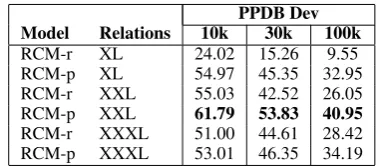
PPDB Dev Model Relations 10k 30k 100k

RCM-r XL 24.02 15.26 9.55

RCM-p XL 54.97 45.35 32.95 RCM-r XXL 55.03 42.52 26.05 RCM-p XXL 61.79 53.83 40.95 RCM-r XXXL 51.00 44.61 28.42 RCM-p XXXL 53.01 46.35 34.19

Table 5: MRR on PPDB dev data for training on an increasing number of relations.

Table 4 shows that all of our models obtain reductions in error as compared to the baseline (cbow), with Joint→RCM obtaining the largest re-duction. This suggests that our embeddings are better suited for semantic tasks, in this case judged by human annotations.

PPDB Dev Model αRCM 10k 30k 100k

Joint-p 1×10−1 _{47.17 36.74 24.50} 5×10−2 _{54.31 44.52 33.07} 1×10−2 _{59.75 50.93 37.73} 1×10−3 _{57.00 46.84 34.45} Table 6: Effect of learning rateαRCMon MRR for

the RCM objective in Joint models.

4.4 Analysis

We conclude our experiments with an analysis of modeling choices. First, pre-training RCM models gives significant improvements in both measuring semantic similarity and capturing human judge-ments (compare “p” vs. “r” results.) Second, the number of relations used for RCM training is an

important factor. Table 5 shows the effect on dev data of using various numbers of relations. While we see improvements from XL to XXL (5 times as many relations), we get worse results on XXXL, likely because this set contains the lowest quality relations in PPDB. Finally, Table 6 shows different learning ratesαRCMfor the RCM objective.

The baseline word2vec and the joint model have nearly the same averaged running times (2,577s and 2,644s respectively), since they have same number of threads for the CBOW objective and the joint model uses additional threads for the RCM objective. The RCM models are trained with sin-gle thread for 100 epochs. When trained on the PPDB-XXL data, it spends 2,931s on average. 5 Conclusion

We have presented a new learning objective for neural language models that incorporates prior knowledge contained in resources to improve learned word embeddings. We demonstrated that the Relation Constrained Model can lead to better semantic embeddings by incorporating resources like PPDB, leading to better language modeling, semantic similarity metrics, and predicting hu-man sehu-mantic judgements. Our implementation is based on the word2vec package and we made it available for general use2_.

We believe that our techniques have implica-tions beyond those considered in this work. We plan to explore the embeddings suitability for other semantics tasks, including the use of re-sources with both typed and scored relations. Ad-ditionally, we see opportunities for jointly learn-ing embeddlearn-ings across many tasks with many re-sources, and plan to extend our model accordingly.

Acknowledgements Yu is supported by China Scholarship Council and by NSFC 61173073.

References

Yoshua Bengio, Holger Schwenk, Jean-S´ebastien Sen´ecal, Fr´ederic Morin, and Jean-Luc Gauvain. 2006. Neural probabilistic language models. In

Innovations in Machine Learning, pages 137–186. Springer.

Yoshua Bengio, Pascal Lamblin, Dan Popovici, Hugo Larochelle, et al. 2007. Greedy layer-wise training of deep networks. InNeural Information Processing Systems (NIPS).

Antoine Bordes, Xavier Glorot, Jason Weston, and Yoshua Bengio. 2012. Joint learning of words and meaning representations for open-text semantic parsing. In International Conference on Artificial Intelligence and Statistics, pages 127–135.

Ronan Collobert and Jason Weston. 2008. A unified architecture for natural language processing: Deep neural networks with multitask learning. In Interna-tional Conference on Machine Learning (ICML). Dumitru Erhan, Yoshua Bengio, Aaron Courville,

Pierre-Antoine Manzagol, Pascal Vincent, and Samy Bengio. 2010. Why does unsupervised pre-training help deep learning? Journal of Machine Learning Research (JMLR), 11:625–660.

Christiane Fellbaum. 1999. WordNet. Wiley Online Library.

Juri Ganitkevitch, Benjamin Van Durme, and Chris Callison-Burch. 2013. PPDB: The paraphrase database. InNorth American Chapter of the Asso-ciation for Computational Linguistics (NAACL). Eric H Huang, Richard Socher, Christopher D

Man-ning, and Andrew Y Ng. 2012. Improving word representations via global context and multiple word prototypes. InAssociation for Computational Lin-guistics (ACL), pages 873–882.

Minh-Thang Luong, Richard Socher, and Christo-pher D Manning. 2013. Better word representa-tions with recursive neural networks for morphol-ogy. InConference on Natural Language Learning (CoNLL).

Tomas Mikolov, Ilya Sutskever, Kai Chen, Greg Cor-rado, and Jeffrey Dean. 2013. Distributed represen-tations of words and phrases and their composition-ality. arXiv preprint arXiv:1310.4546.

Andriy Mnih and Geoffrey Hinton. 2007. Three new graphical models for statistical language modelling. In International Conference on Machine Learning (ICML).

Andriy Mnih and Yee Whye Teh. 2012. A fast and simple algorithm for training neural probabilistic language models.arXiv preprint arXiv:1206.6426. Robert Parker, David Graff, Junbo Kong, Ke Chen, and

Kazuaki Maeda. 2011. English gigaword fifth edi-tion. Technical report, Linguistic Data Consortium.

Deepak Ravichandran, Patrick Pantel, and Eduard Hovy. 2005. Randomized algorithms and nlp: us-ing locality sensitive hash function for high speed noun clustering. In Association for Computational Linguistics (ACL).

Richard Socher, Alex Perelygin, Jean Wu, Jason Chuang, Christopher D. Manning, Andrew Ng, and Christopher Potts. 2013. Recursive deep models for semantic compositionality over a sentiment tree-bank. InEmpirical Methods in Natural Language Processing (EMNLP), pages 1631–1642.

Joseph Turian, Lev Ratinov, and Yoshua Bengio. 2010. Word representations: a simple and general method for semi-supervised learning. In Association for Computational Linguistics (ACL).