A reduced uncertainty hybrid evolutionary algorithm for solving dynamic shortest path routing problem

http://wrap.warwick.ac.uk

Original citation:

Kusetogullari, Huseyin, Sharif, Haidar, Leeson, Mark S. and Celik, Turgay. (2015) A

reduced-uncertainty hybrid evolutionary algorithm for solving dynamic shortest-path

routing problem. Journal of Circuits, Systems and Computers, 24 (5).

Permanent WRAP url:

http://wrap.warwick.ac.uk/73771

Copyright and reuse:

The Warwick Research Archive Portal (WRAP) makes this work by researchers of the

University of Warwick available open access under the following conditions. Copyright ©

and all moral rights to the version of the paper presented here belong to the individual

author(s) and/or other copyright owners. To the extent reasonable and practicable the

material made available in WRAP has been checked for eligibility before being made

available.

Copies of full items can be used for personal research or study, educational, or not-for

profit purposes without prior permission or charge. Provided that the authors, title and

full bibliographic details are credited, a hyperlink and/or URL is given for the original

metadata page and the content is not changed in any way.

Publisher’s statement:

Electronic version of an article published as Journal of Circuits, Systems and

Computers, 24 (5). 10.1142/S021812661550067X © World Scientific Publishing

Company

http://0-www.worldscientific.com.pugwash.lib.warwick.ac.uk/worldscinet/jcsc

A note on versions:

The version presented here may differ from the published version or, version of record, if

you wish to cite this item you are advised to consult the publisher’s version. Please see

the ‘permanent WRAP url’ above for details on accessing the published version and note

that access may require a subscription. For more information, please contact the WRAP

A reduced uncertainty based hybrid evolutionary algorithm for solving dynamic shortest-path routing problem

Huseyin Kusetogullari

Department of Computer Engineering, Gediz University, Seyrek, Izmir, Turkey

Md. Haidar Sharif∗

Department of Computer Engineering, Gediz University, Seyrek, Izmir, Turkey

Mark S. Leeson

The School of Engineering, Warwick University, Coventry, UK

T. Celik

School of Computer Science, University of the Witwatersrand, Johannesburg, South Africa

Received (July 7, 2014) Revised (December 17, 2014)

Accepted (Day Month Year)

The need of effective packet transmission to deliver advanced performance in wireless networks cre-ates the need to find shortest network paths efficiently and quickly. This paper addresses a Reduced Uncertainty Based Hybrid Evolutionary Algorithm(RUBHEA)to solve Dynamic Shortest Path Rout-ing Problem(DSPRP)effectively and rapidly. Genetic Algorithm(GA)and Particle Swarm Optimiza-tion(PSO)are integrated as a hybrid algorithm to find the best solution within the search space of dynamically changing networks. Both GA and PSO share context of individuals to reduce uncertainty in RUBHEA. Various regions of search space are explored and learned by RUBHEA. By employing a modified priority encoding method, each individual in both GA and PSO are represented as a potential solution for DSPRP. A Complete statistical analysis has been performed to compare the performance of RUBHEA with various state-of-the-art algorithms. It shows that RUBHEA is considerably supe-rior (reducing the failure rate by up to 50%) to similar approaches with increasing number of nodes encountered in the networks.

Keywords: Shortest path, encoding, decoding, uncertainty reduction, genetic and hybrid algorithms.

1. Introduction

Dynamic Shortest Path(DSP) routing has become a critical and key element in routing protocols to improve the utilization of wireless communication networks. Routing data packets through DSP is normally deemed as an efficient approach to increase the perfor-mance of wireless network utilization since it minimizes cost or delay while maximizing

quality. Shortest-path routing is also a markedly notable technique for newly emerging technologies, chiefly video-conferencing and video on demand which require high band-width, low delay, and low delay jitter1_{. DSP discovery in a more efficient and faster}

manner is a challenging problem in mobile ad hoc networks, wireless sensor networks, etc. Variations of DSPRP have to be solved to gain high throughput communication in a wide variety of network problems e.g., multi-shortest-path2, constrained shortest-path3, multi-objective shortest-path4_{, DSP discovery}5_{, and travelling salesman problems}6_{. Most}

of these problems are non-polynomial hard and one way of solving them is to assign a cost metric (weight) for each link in the network. To date a range of deterministic algorithms e.g., Dijkstra’s algorithm7_{, breadth-first search algorithm}8_{, and Bellman-Ford algorithm}9

have been developed to find the lowest cost or shortest-path routing from a source to a given destination through a network. However, they have limits such as being inflexible or lacking the adaptability needed to achieve shortest-path in rapidly changing network topologies10,11,12_{. So it is eminent to employ proper new approaches for solving DSPRP}

rapidly and efficiently10,11,12_.

Evolutionary algorithms have drawn considerable attention as DSPRP solvers since they provide a more robust and efficient approach to solve such complex problems10,13,14,15,16. GA10, genetic programming17, and evolutionary programming18 have been proposed for various network problems. The algorithm of Ji et al.19_integrated

stochastic simulation and GA to solve the shortest path problem with stochastic arc length. Vijayalakshmi et al.20 _{proposed a GA based hybrid algorithm for multi-cast routing in}

which the crossover and mutation operators have been refined for solving the multi-cast routing problem. An improved hybrid algorithm which applies in multi-cast routing to provide effective solutions for a complex quality of service problem has been proposed by Wang et al.21. El-Mihoub et al.22showed the combined effect of the probability of local search and the learning strategy on the population size requirements of a hybrid algorithm. Incorporation of more than two algorithms was developed by Potter et al.23but the algo-rithmic complexity was greatly increased over a two element solution. Work employed a GA based on variable-length chromosomes to construct a routing table that is a population of strings with each one represents a route. An improved GA was investigated to opti-mize DSPRP by Yang et al.24_{. In addition, neural networks have also got a great deal of}

popula-tion is generated from the current populapopula-tion which involves weak and strong candidates. The weak candidates undergo more corrections than the strong ones to overcome values at which the algorithms become stuck (local optima) or (occasionally) assist the strong ones to reach a global optimum. Numerous practical approaches can be carefully weighed to overcome stuck values or local minima in meta-heuristic algorithms such as increasing the number of iterations or using a larger population size, which increase both the memory requirements and the route computation time. Also these strategies are very basic and not largely effective in resolving a search space problem. Both GA and PSO have a solution from different perspectives since GA works based on the mechanism of natural selection as well as evolutionary genetics and PSO works based on social adaptation of knowledge. Hence, singly applied algorithms have not provided much opportunity for exploring the global optimum in the different regions of search space. Thus hybrid of GA and PSO plays a vital role to solve many real-world optimization problems.

A comparison of the PSO-based search algorithm and a GA for solving DSPRP is pro-posed by Mohemmed et al.29_{. A priority-based indirect path-encoding scheme is used to}

widen the scope of the search space, and a heuristic operator is used to reduce the proba-bility of invalid loop creations during the path-construction procedure. Authors29_claimed

that PSO-based algorithm was superior to that using GA for finding DSP in dynamically changed networks. Moreover, PSO has been applied inter alia to several applications in the fields of evolutionary computing and optimization30,31. Juang12presented a Hybrid of GA and PSO(HGAPSO), an evolutionary learning algorithm, for recurrent fuzzy network design. In the algorithmic steps, GA and PSO work with the same population which means that the top 50% of individuals are evaluated and enhanced by using the operators of GA and PSO. Ji19 _{proposed a hybrid intelligent algorithm which was integrating stochastic}

simulation and GA to solve the shortest-path problem with stochastic arc length. Mari-nakis et al.6_{addressed a Hybrid of Genetic Algorithm and Particle Swarm Optimization} (HybGENPSO)for the vehicle routing problem. In the algorithmic steps, randomly created individuals are first placed in a population pool, and then the operators of GA and PSO are respectively applied to the individuals to produce the new generation. The authors6_claimed

that by the effect of PSO the use of an intermediate phase between the two generations will give more efficient individuals and, henceforth, will improve the effectiveness of the al-gorithm. A hybrid algorithm based on ant colony optimization with scatter search was implemented for the vehicle routing problem in the field of distribution and logistics25_,

delivering higher performance solutions relative to other competing heuristics.

In spite of different efforts the desired level of efficiency and rapidity in DSPRP algo-rithms did not come along. To solve DSPRP efficiently and rapidly a bit more, we have de-veloped a new reduced uncertainty based hybrid evolutionary algorithm (RUBHEA) which is a hybrid of GA and PSO. From a given dynamically changing network model, RUBHEA finds a set of dynamic paths with their cost values which are then evaluated for obtaining the dynamic shortest-path as a final result quickly and efficiently.

between GA and PSO. Candidates in the sub-populations will be exchanged to compose the new sub-populations and the solution strategy will avoid the need to change the pa-rameters of the operators in the algorithms for finding the global optimum. (ii) RUBHEA learns DSPRP and reduces the uncertainty in the problem. It adopts the modified search based priority encoding method to represent a path in an undirected network. Multiple comparisons without statistical tests and with statistical tests considering various scales of networks illustrate the effectiveness and the efficiency of RUBHEA by comparing with the existing state-of-art dynamic shortest-path routing algorithms based on GA (e.g., Ahn et al.10), PSO (e.g., Mohemmed et al.29), as well as hybrid of GA and PSO (e.g., Juang et al.12_{and Marinakis et al.}6_).

The rest of the paper is organized as follows. List of acronyms and symbols used in this paper will be demonstrated in section2. DSPRP problem will be defined in section3. Existing approaches for finding shortest-path will be explained in section4. The proposed approach RUBHEA for finding shortest-path will be presented in section5and, thereafter, the modified version of encoding method for solving DSPRP will be discussed. Results and discussions will be provided in section6, and finally the paper will be concluded in section7.

2. Glossaries

A lot of acronyms and symbols have been used in this paper. In this section, we have demonstrated those acronyms and symbols so that readers can easily follow them through-out the paper.

Acronyms

DSPRP Dynamic Shortest Path Routing Problem.1–5,7,9,11,12,16,19,21,25,31,32

DSP Dynamic Shortest Path.1–3,6,7,9,16,20,21,29

GA Genetic Algorithm.1–4,7–13,15–18,20–22,26,31,32

HGAPSO Hybrid of GA and PSO.3,20,26,30,31

HybGENPSO Hybrid of Genetic Algorithm and Particle Swarm Optimization.3,20,21,26,30,31

PSO Particle Swarm Optimization.1–4,7,10–13,15–17,20–22,26,31,32

RUBHEA Reduced Uncertainty Based Hybrid Evolutionary Algorithm.1,3–7,11–26,29–32

List of Symbols

C(cg_k

1) Fitness value of individualk1in the GA at iteration numberg.15

C(cg_k

3) Cost value of selected weaker chromosomek3at iteration numberg.15

C(pg_k

2) Fitness value of individualk2in the PSO at iteration numberg.15

C(pg_k

3) Fitness value of selected fitter particlek3at iteration numberg.15

D Destination node.5,9

E(t) Set of time varying links at timet.4,5,13

H(x) Entropy ofxat particular instance ofX.6

H(y\x) Relationship between past and future network topologies.7

IDs Identities of nodes.7,13,16

Ii,j(t) Link connection indicator between nodesiandjat timet.6,9

Ii,j(t+ 1) Link connection indicator between nodesiandjat timet+ 1.9

Ij,i(t+ 1) Link connection indicator between nodesjandiat timet+ 1.9

J Algorithm for describing behaviors of nodes and links versus time.4

N(t) Set of time varying nodes at timet.4,5,13

N Total number of observations.27,28,30–32

P(cg_k

1) Probability of occurrence of chromosomek1at iteration numberg.15

P(pg_k

2) Probability of occurrence of particlek2at iteration numberg.15

P(qt

i) Probability ofqitinQt.6,7

P(qt_i+1\qt

i) Probability ofq t+1

i \qit.7

Qt _{State space at timet.6,7}

Qt+1 _{State space at timet+ 1.7}

Ri,j(t) Estimation learned about the least cost to reach destination node at timet.9

S Source node.5,9

W(t) Set of time varying cost values over links at timet.4,5,13

Wi,j(t+ 1) Cost value associated with each link(i, j)at timet+ 1.9

X A random process.6

Y Next random process.7

` Randomly selected point in the chromosome.8

Independent population data set.15

η Intersection value.12–15,17,21–26,29–32

γg _{Number of discarded candidates at iterationg.12}

µg₁ The mean of cost values of population in the GA at iteration numberg.15

µg2 The mean of cost values of population in the PSO at iteration numberg.15

µg₃ The mean of fitness values of population in the RUBHEA at iteration numberg.15

ω Inertia weight.10,11,13

ρg _{Sub-population size at iterationg.12,15}

σg₁ The standard deviation of cost values of population in the GA at iteration numberg.15

σg₂ The standard deviation of cost values of population in the PSO at iteration numberg.15

σg₃ The standard deviation of fitness values of population in the RUBHEA at iteration numberg.15

τt

n nthnode inN(t).5

~

υk Velocity vector of individual particlek.10,12,13

~

xgbest _{Global best position in the search space.10}

~

xk Position vector of individual particlek.10,12,13

~ xbest

k Personal best position of individual particlekin the search space.10

~

za athchromosome.8

~

c1, c2 Two learning factors in the PSO.10,11,13

d Dimensional search space.8,10,13

et

m mthlink inE(t).5

f(t) :J Mapping function.4,5

fgbest _{Global best objective function’s value.10}

fk Objective function value of particlek.10

fbest

k Personal best value of individual particlek.10

g Generation index.10,12,13,15

i, j Pair of selected two nodes.6,9

k3 Individual particle and chromozome in the RUBHEA.15

kc Number of chromosomes.13,15

kp Number of particles.10,13,15

k Particle number in the PSO.10

m+ _{Convergent value.15}

n Number of nodes in network.6,10,13

pc Crossover rate.8,13,20

pm Mutation rate.8,13,20

qt β β

th_{element inQ}t_.6

r, s Randomly selected two crossover points.8

t Time or step number.6,7,9

u1, u2 Uniformly distributed two random variables.11,13

x Particular instance ofX.6

y Particular instance ofY.7

3. Problem Definition in Dynamic Network Models

In this section, we have focussed on the explanation of dynamically changing networks followed by DSPRP as well as the measurements of uncertainty and entropy in dynamic network models.

3.1. Dynamically changing networks

A complete definition of networkG(t)must include both structural and behavioural infor-mation so the definition of dynamic network model is:

G(t) ={N(t), E(t), W(t), f(t) :J}, (1)

as time passes in a network. In this sense, a network is a dynamic. For instance, the shape of a network, as defined by behaviors and the mapping function f(t) :J, may change as links are dropped, added, or rewired (switched from one node to another) over time. It changes based on the movement and transmission range of the nodes in net-work topologies. Besides this,W(t)has changed over time. Furthermore, a network may grow with the addition of nodes and links over time. LetN(t) ={τt

1, τ2t, τ3t, . . . , τnt}and E(t) = {et

1, et2, et3, . . . , etm} ⊆N(t)×N(t)be a set of nodes and a set of arcs,

respec-tively. We assume thatN(t)andE(t)are finite sets. LetS andDbe two nodes ofN(t) such thatS 6=D. Thus, one of the possible paths from sourceSto destinationDmay be represented as{S, τt

1, et1, τ2t, et2, . . . , D}, respectively. However, many different paths can

be obtained from source node to destination node in the network topology so the uncer-tainty in network topologies should be reduced for finding the shortest path rapidly and efficiently.

3.2. DSPRP

A network graph is a collection of vertices and edges randomly connecting them pair-wise. Network graphs can be static or dynamic. In the static graph the number of nodes and links, the shape of the mapping function and other properties of graphs remain the same whereas in the dynamic graph they may change over time32. Therefore, it is very hard to resolve dynamically changing graphs compared to the static network graphs. In dynamically change networks, finding shortest path is a very complex problem as it is nec-essary to compute the costs of all maintained paths between source and destination nodes. By applying the proposed method RUBHEA, we will prevent recomputing all paths once we obtain the dynamic shortest routing path. There are many research efforts reported in the literature of maintaining shortest paths on dynamic graphs. For examples, Dijkstra’s algorithm7, breadth-first search algorithm8, and Bellman-Ford algorithm9 had been pro-posed and improved to obtain the shortest-path routing from a source node to a destination node in networks. These algorithms are very inefficient when the occurrence of link state changes in a network. Some other methods maintain shortest paths in Hypergraphs33_{, in}

planar graphs32,34, some require un-weighted graphs35, and some permit only integer edge weights36,37_{, and its variant}38_{. Many other shortest path problems have been solved by}

us-ing different approaches39,40,40,41,42,43_{. In this work, we have focused on developing a}

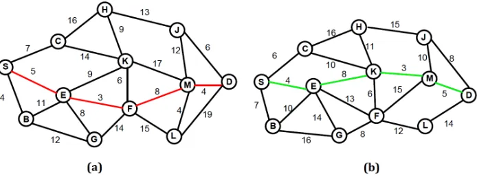
Fig. 1. Example of a small dynamically changing network model.

communication. To find the dynamic shortest path, each edge between the pair of nodes is assigned with an independent weight value as shown over the edges in Fig.1. By using RUBHEA the dynamic shortest path (S-E-F-M-D) shown by the red line is obtained in Fig.1(a). After the weights of the edges are changed in the network model, the costs of all paths between source and destination nodes are recomputed and a new shortest path (S-E-K-M-D) is found as shown by the green line in the Fig.1(b).

3.3. Uncertainty and entropy measurements in dynamic networks

Uncertainty in dynamically changing network topology has the considerable effect on find-ing DSP. It should be as small as possible to obtain DSP or solve the optimization problem rapidly and efficiently. Otherwise, it will be extremely complex problem for efficient solu-tion. For instance, finding DSP in a dynamically changing network is a very hard problem because of the movement of the nodes and variations of the connectivity between nodes. To offer a great solution for the complexity problem, uncertainty is reduced both in the dy-namically changed network topologies and in the hybrid algorithms. A network ofnnodes is defined by the set of indicator variablesIi,j(t)for i, j ∈ 1,2,3, ..., n. We note that a

node cannot be adjacent to itself which means that a node cannot transmit a message to it-self and it is described asIi,j(t) = 0for alli=j. An adjacent matrix represents the entire

connectivity of the network topology at timet. The set of allowable configurations of that

adjacent matrix forms a state spaceQt ₌n_qt

1, qt2, qt3, ..., qtβ

o

whereβ = 2n(n−1)/2_{. Let} Xbe a random process denoting the trajectory of the networks topology through the state spaceQtand letxdenote a particular instance ofX, then the information entropy44,45can be estimated as:

H(x) =− X

qt

i∈Qt

P(q_it)log2P(qti) (2)

whereP

qt

i∈Qtp(q

t

i) = 1. IfP(q

t

i) = 0for somei, the value of the corresponding

sum-mand0log20is taken to be 0.H(x) = 0signifies that there is no uncertainty and

The main advantage of the proposed method is that it learns and reduces the uncer-tainty during iterations. On estimating DSP at timet, the connectivity between nodes in the network topology and adjacent matrix may change. The relationship between past and future network topologies is stated as follow:

H(y\x) =− X

qt

i∈Qt

P(q_it) X

qt_i+1∈Qt+1

P(qt_i+1\qt_i)log2 1

P(q_it+1\qt i)

) (3)

whereY is a random process denoting the trajectory of the new network topology through the state spaceQt+1andydenotes a particular instance ofY. In Eq.3, the relationship be-tween past and future network topologies can be clearly analysed. For instance, the entropy of the unknown result of DSP is minimum in the network topology at time(t+ 1)since

H(y\x) = 0. This outcome proves that the new network topology is completely same

with the past network topology. On the other hand, the adjacent matrices of past and future network topologies are examined and compared to find the amount of the changes between the network topologies in the situation of maximum uncertainty as it is most difficult to predict the outcome of DSP. As a result, continuously changing problem becomes easier to be solved by decreasing the uncertainty from the known information and the proposed search space algorithm tries to find the new global optima only in the part of the network topology changed.

4. Existing Approaches for Finding Shortest-path

Ahn et al.10_{and Mohammed et al.}29_{demonstrated the effectiveness of using GA and PSO}

algorithms for finding shortest path in communication networks respectively. In this sec-tion, existing shortest path algorithms which are GA10and PSO29to find shortest path will be clearly explained. In the next section, the proposed method which is reduced uncertainty based hybrid evolutionary algorithm RUBHEA will be presented to compute the shortest path in dynamically changing networks.

4.1. GA Approach

In the standard GA method10_{, a number of candidate solutions (chromosomes or}

popula-tion) are randomly generated with each one consisting of a fixed number of variables called genes or priority of nodeIDs. And then the chromosomes are examined to find the opti-mal solutions (fitness values) according to the given objective function. Priority values of genes are reflected in the nodeIDsof the chromosome which represents an order of nodes in a routing path. Each chromosome should not exceed the total number of nodes in the network. The gene of the first node ID is specified as a source node and other nodes of the chromosome are selected randomly or heuristically until the destination node is reached. Thus a routing path is constructed as a potential solution.

known as parents and the results in new chromosomes known as offspring. Stochastic se-lection operators are effective approaches for choosing which (fitter) chromosomes will survive because they will have a higher chance of being selected than less fit ones. Nev-ertheless, even the weak chromosomes typically have a chance to become a parent or to survive. Sometimes individuals may rapidly come to dominate the population causing con-vergence to a local minimum. To avoid this, a larger population with a modest crossover ratepc but a relatively high mutation ratepmwill cause rapid convergence to the known

optimum solution and results in one new chromosome. Applying crossover and mutation leads to a set of new offspring chromosomes. Based on their fitness, these compete with the old chromosomes for a place in the next generation. This complete process can be iterated until an optimal fitness value is estimated or a previously set time limit is reached.

4.1.1. Offspring generation operators

Crossover and mutation operators are the major evolutionary and distinguishable operators of GA. Crossover operates on two chromosomes at any iteration number and creates off-spring by combining genes of both chromosomes. Thus there is a transfer of information or genes between the candidates/individuals that created offspring/offsprings collect the beneficial information to find better result. The most known and used crossover operators are partial-mapped crossover, order crossover, cycle crossover, position-based crossover, heuristic crossover10,24_{. In the crossover method, the most significant point is to define}

a proper crossover operator for the corresponding problem since it plays a major role in GA to achieve a better performance. Consider two different individuals~za and~zb ind

-dimensional search space of the given population, i.e.,

~

za =za1, za2, ..., zar, ..., zas, ..., zad ~

zb=zb1, zb2, ..., zbr, ..., zbs, ..., zbd

(4)

wherer, sdenote two randomly selected crossover points denote two randomly selected crossover points, andr < s. After the crossover operator employed, the produced individ-uals or new candidate solutions become

~za=za1, za2, ..., zbr, ..., zbs, ..., zad ~

zb=zb1, zb2, ..., zar, ..., zas, ..., zbd.

(5)

Crossover probability determines the number of offspring individuals produced. Unlike the crossover, mutation is an operator which produces random changes of genes in var-ious chromosomes. Mutation serves the crucial role of either replacing the genes lost from the population during the selection process so that they can be tried in a new con-text or providing the genes that were not present in the initial population. Let us suppose

~za =za1, za2, ..., za`, ..., zadwhere`denotes the randomly selected point in the

chromo-some. Consequently,`th_genez

a`of the individual can be changed or mutated to produce

the offspring will start to lose their resemblance to the ability to learn from the history of the search.

4.1.2. Selection operator and fitness function

Major role of applying the selection operator is to improve the quality of generated population. Roulette wheel selection operator is an effective approach to choose fitter chromosomes46. Fitter chromosomes will have a higher chance of being selected than less fit ones46_{. Nevertheless, even the weak chromosomes typically have a chance to become}

a parent or to survive. Superior individuals should have more opportunities to produce the next generation because they have a higher probability of reaching the feasible solution. In this work, Roulette wheel selection operator is used for choosing two fitter chromosomes from the population to create offspring. In a GA, the quality of a represented chromosome or potential solution is estimated by a fitness function, whose purpose is to map a chromo-some representation into a scalar value or a cost value. For the DSP routing problem, the fitness function estimates a cost value for each chromosome that is based on the distance to the global optimum. Hence strong and weak candidates can be evaluated according to their fitness values and multiple offspring are produced based on them.

LetSandDdenote source and destination nodes, respectively andIi,j(t)be the link

connection indicator between nodesi andj which plays the role of a chromosome map providing information on whether the link from nodeito nodej is included in a routing path or not at timet, i.e.,

Ii,j(t) =

  

1,if the link from nodeito nodej

exists in the routing path; 0,otherwise.

(6)

The classical fitness function10,29has been modified to solve the DSPRP as:

D

X

i=S D

X

i=S j6=i

Wi,j(t+ 1)·Ii,j(t+ 1) +Ri,j(t)·Ii,j(t)) (7)

D

X

i=S j6=i

Ii,j(t+ 1)− D

X

i=S j6=i

Ij,i(t+ 1) =

  

1,ifi=S;

−1,ifi=D; 0,otherwise.

(8)

D

X

i=S j6=i

Ii,j(t+ 1) =

≤1,ifi6=D;

0,ifi=D, (9)

whereIi,j(t+ 1)∈ {0,1},∀i, jandRi,j(t)is the estimation learned about the least cost

to reach destination node from nodeito nodej. The value ofRi,j(t)is0sinceH(y\x) =

4.2. PSO Approach

PSO algorithm is a relatively new optimization algorithm which inspired by social behavior of colony of animals in environment28. Like GA, the PSO is a population-based optimiza-tion method that searches multiple soluoptimiza-tions29,30,25_{. However, PSO employs a different}

strategy unlike GA, which utilizes a competitive strategy. The search for an optimal posi-tion (soluposi-tion) is performed by updating the particle velocities in each iteraposi-tion/generaposi-tion according to their fitness values, estimated by using the fitness function. If the fitness value does not provide the optimum solution, the position of the following properties of an indi-vidual particlekis updated in the following way in each iteration. Ind-dimensional search space, current position of particlekis denoted by~xk, the corresponding objective

func-tion value byfk, the current velocity of particlekby~υk, and the personal best position

and global best position in search space by~xbest k and~x

gbest_{, respectively. The personal}

best position,~xbest

k , corresponds to the position in search space where particlekhad the

smallest valuefbest

k as determined by the objective function. Meanwhile, the global best

position~xgbest represents the position yielding the current global best objective function valuefgbest_{amongst the entire particles’ best positionsf}best

k . Eqs.10and11define how

the velocities and locations of swarm particles are updated at iterationg, respectively. As a summary, the PSO28_{performs the following steps:}

(1) Initialize the number of particleskp, generation indexg, constantsc1, c2.

(2) Randomly initialize particle positions~xk =xk1, xk2, . . . , xkd.

(3) Randomly initialize particle velocities~υk =υk1, υk2, . . . , υkd,0 ≤υko ≤υmaxfor o= 1,2, . . . , nwhereυmaxis a constant.

(4) Evaluate fitness valuesfk:

if fk < fkbestthenf best

k =fk,~xbestk =~xk

if fk < fgbestthenfgbest=fk,~xgbest=~xk.

(5) Update all particle velocities~υkusing Eq.10.

(6) Update all particle positions~xkusing Eq.11.

(7) Setg←g+ 1, check termination criterion. If termination criterion satisfied stop and produce results else return to step 4.

PSO explores addimensional space, using a population of particles which are initially pro-vided with random velocities and positions in the problem space. Each particle represents a candidate solution to the problem. The particles change their positions by moving around the search space until a relatively unchanging arrangement has been encountered, or the stop criterion is satisfied. Each particle changes its position according to its best velocity and all particles’ best velocity or global best velocity. In this case, each particle’s position will change to attain its own best result according to its best velocity and attempt to find the global optimum according to the best velocity of particles thus

~

υk ←ω~υk+c1u1 ~xbestk −~xk

+c2u2 ~xgbest−~xk

(10)

~

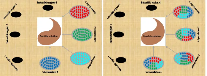
Feasible solution Feasible solution

Fig. 2. Schematic diagram of different sub-population interaction strategy to approach to the feasible solution.

{u1, u2} ∈ [0,1]are uniformly distributed random variables andc1, c2 are two learning

factors that controls the influence of personal best and global best in the search process. In PSO, bothc1andc2are chosen between[0,4.0]to deliver good results29. Inertia weightω

is selected randomly between[0,1]in each generation.

5. The Proposed Approach RUBHEA for Finding Shortest-path

In this section, we have discussed our proposed approach RUBHEA for finding shortest-path from a continuously changing network model.

5.1. Algorithm of RUBHEA

RUBHEA consists of GA and PSO to solve DSPRP more efficiently and rapidly in a con-tinuously changing network topology. It learns the estimations by reducing the uncertainty in the problem and in the algorithm itself, iteratively. Each node has estimation of the short-est path length (cost) to the dshort-estination node which should be learned and updated, and also the node learns the estimated cost of its edges to the neighbors. RUBHEA is employed by letting the operators of GA and PSO run simultaneously until an optimal fitness value is estimated or a previously set iteration limit is reached. During each iteration, RUBHEA shares information by each informing the other of their respective optimum values in their own sub-populations and consequently uncertainty is reduced. In the Fig.2 for the first iteration the estimated shortest path lengths (costs) in the subpopulation 1, subpopulation 2, subpopulation 3, and subpopulation 4 are symbolized as•,•,•, and•, respectively. For the second iteration the estimated shortest path lengths (costs) in the subpopulation 1, sub-population 2, subsub-population 3, and subsub-population 4 are obtained by sharing estimated•,•,

•, and•to get a feasible solution.

be shared depends on the current best optimum fitness value of all candidates. Assume that a chromosome reaches the best fitness value compared with all other chromosomes and particles. This shows that GA is closer to the global optimum than PSO and particles start to search around the current optimum result. As a result strong chromosomes are sent into the population of PSO and replaced with weak particles. And there will be a new population which is a combination of particles and strong chromosomes and they will be merged by using PSO operators to obtain better result in the next iteration. Henceforth, reducing uncertainty in two efficient meta-heuristic algorithms will make RUBHEA more efficient in resolving the DSPRP. To perform the RUBHEA, fittest members of popula-tions from different meta-herustic algorithms are evaluated and the populapopula-tions with less fit members are modified by injecting fittest members of other populations resulted from different meta-herustic algorithms. Meanwhile, less fit members of updated populations are discarded. Therefore, the following constraints between GA and PSO must be satisfied:

ρ(g+1)_=ρg_−γg_+ρg_×η=ρg_{(1 +η)−γ}g ₍₁₂₎

withρg×η≤γgwhereη∈[0,1]as well asρgandγgdenote the sub-population size and the number of discarded candidates at iterationg, respectively.

In this paper, we have assumed that the number of discarded candidates is equal to number of join candidates. The intersection percentage of candidatesηhas been applied to keep the population size constant for each meta-heuristic algorithm and the candidates in each algorithm will be merging to approach to the global optimum effectively. Step-by-step procedure for RUBHEA has been stated in Algorithm1.

5.2. Time complexity of RUBHEA

Typically, the computational complexity analysis is involved in the complexity of the prob-lem over all possible instances, sizes, and algorithms. The number of computations re-quired for a complete run of the PSO are the sum of the computations rere-quired to calculate the cost of a candidate solution based on Eq.7and the computations required to update each particle’s~xk and~υk based on Eqs. 10and11. These estimations are directly

Algorithm 1RUBHEA(G(t),η). Algorithm of RUBHEA for solving dynamic shortest-path rout-ing problem from a given network.

Input:G(t) = (N(t), E(t), W(t)), ηwhereN(t)⇒set of time varying nodes in a given network modelG(t),E(t)⇒set of time varying links inG(t), andW(t)⇒set of time varying links’ weight values inG(t).

Output:Best fitness value and shortest-path.

1: Initializekp,kc,pc,pm,~xk,~υk,ω,u1, u2,c1, c2,g,d=n.

2: Set the source and destination nodeIDs.

3: Randomly initialize the populations of particles and chromosomes.

4: Use local search based encoding method on chromosomes and particles to represent valid paths.

5: Evaluate the fitness values of all individuals by applying Eq.7. 6: ifthe fittest value of all candidates is estimated from a particlethen

7: Apply Eqs.7and12for selecting the fitter particles and the weaker chromosomes. 8: Reduce Uncertainty in sub-population of GA.

9: end if

10: ifthe fittest value of all candidates is estimated from a chromosomethen

11: Apply Eqs.7and12for selecting the fitter chromosomes and the weaker particles. 12: Reduce Uncertainty in sub-population of PSO.

13: end if

14: Apply operators of GA and PSO for each chromosome and particle, respectively. 15: ifthe optimal value is not estimated or a previously set iteration limit is not reached

then

16: Repeat from step 4. 17: end if

18: return

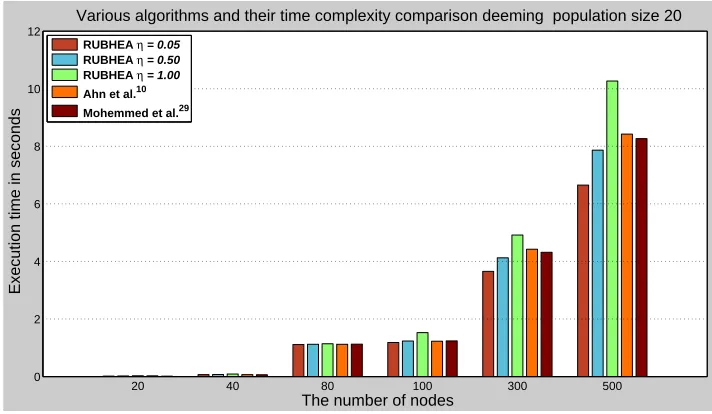
Fig.3depicts the comparison of the average execution time of the algorithms required to achieve the results as shown in Fig.11, where the population size in the algorithms is 20. The implemented algorithms have been used to obtain the shortest-path in the given six different network models. For less than 80 nodes, the average execution time required for PSO proposed by Mohemmed et al.29_{is less than the other shortest-path algorithms.}

For the greater network models, the proposed method RUBHEA withη = 0.05provides the best average execution time compared to the other algorithms and it takes average of 1.113, 1.183, 3.653 and 6.653 seconds for execution to find the shortest-path in 80, 100, 300, and 500 nodes, respectively.

We have calculated the speedup47 of various algorithms with respect to the genetic algorithmic approach of Ahn et al.10, which solves the shortest path routing problem. Speedup has been defined as the ratio of the execution time of the algorithm of Ahn et al.10

The number of nodes

Execution time in seconds

Various algorithms and their time complexity comparison deeming population size 20

20 40 80 100 300 500

0 2 4 6 8 10 12

RUBHEA η = 0.05

RUBHEA η = 0.50

RUBHEA η = 1.00

Ahn et al.10

Mohemmed et al.29

Fig. 3. Comparison of the execution time with various algorithms for six different network models.

The number of nodes

Speedup

Speedup with respect to the algorithm of Ahn et al.10 deeming population size 20

20 40 80 100 300 500

0 0.2 0.4 0.6 0.8 1 1.2 1.4 1.6 1.8

RUBHEA η = 0.05

RUBHEA η = 0.50

RUBHEA η = 1.00

Mohemmed et al.29

Fig. 4. Speedup with respect to the algorithm of Ahn et al.10_.

5.3. Uncertainty reduction in RUBHEA

As it is known, the strong candidates have more chance than the weak candidates to reach to the global optimum according to the estimated cost values (fitness values)48. Zhang et al.46 _{discussed adaptively changing the probabilities of mutation and crossover in each}

generation based on the probability distribution of population. Let P(cg_k

1) and P(p

g k2)

be the probability of occurrence of chromosomek1 ∈ {1,2,3, ..., kc} and particlek2 ∈

{1,2,3, ..., kp}at generationg andC(c g

k1)andC(p g

k2)be the corresponding cost values

(fitness values) in GA and PSO, respectively. The mean and standard deviation of cost values of populations denoted asµg₁ andσ₁g for GA as well as µg₂ andσ₂g for PSO are defined as follows:

µg₁ =

kc

P

i=1

P(cg_i) lim

λ→m+(C(c g

i)−λ) µ

g

2=

kp

X

j=1

P(pg_j) lim

λ→m+(C(p g j)−λ)

(13)

σ₁g= s

kc

P

i=1

P(cg_i)[µg₁−C(cg_i)]2 _σg

2=

s

kp

P

j=1

P(pg_i)[µg₂−C(pg_j)]2 ₍₁₄₎

wherem+is defined as the convergent value. In RUBHEA, uncertainty reduction strategy is depending on the best fitness value of overall candidates in GA and PSO. If the best fitness value is found from a chromosomes, then a number of selectedρg_{×ηchromosomes}

will replace with selected weak particles into the population of PSO. On the other hand, if the best fitness value is estimated from a particle then, a number of selectedρg_{×ηparticles}

will replace with the selected weak chromosomes into the population of GA.

LetC(pg_k3)andC(cg_k3)be the cost values of selected fitter particles and weaker chro-mosomes at generationg,k3 ∈ {1,2, . . . , n3=ρg×η}, respectively. After this

interac-tion, theµg₃andglsσ₃gwill be formulated in RUBHEA as follows:

µg₃ = _n1

3 kcµ

g

1−

kc−ρgη

P

i=1

C(pg_i) +kpµg2−

ρg_η

P

j=1 C(cg_i)

!

,

σg₃ = s 1 n3 n3 P i=1

(µg₃−C(pg_i))2+ (µg₃−C(cg_i))2.

(15)

Generally, the interaction ofnindependent population data set=1, 1, . . . , nwill be

formulated as follows:

µg

=

P

iniµi

P

ini σ

g

=

qP

ini(σi2+µ

2

i)

P

ini −µ

g

2

i∩j=∅ ∀i6=j. (16)

The means and standard deviations of all sub-populations are estimated in each gener-ation/iteration and they will be used to estimate the variation of new population which is consisted of chromosomes and particles. By estimatingµ3andσ3in RUBHEA, the

proba-bility of reaching to the global optimum will be increased because theσ3will be decreased

candidates to find global optima or DSP routing in short time will be achieved after inter-secting the sub-populations in two effective algorithms.

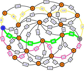
With regard to the development of an effective algorithm for solving search space prob-lems, there are two possibilities that render the proposed approach remarkable and signifi-cant. One is to share information (priorities of nodeIDs) between two effective algorithms and the second is to apply the operators of algorithms to the mixed individuals informa-tion. The strategy of our proposed method and performance and influence of GA operators in RUBHEA are illustrated in an example10,29of the undirected graph shown in Fig. 5

which has 20 nodes and 48 edges. The optimal paths shown in Fig.5with yellow and pink solid lines are estimated as optimal paths of GA (path⇒A-E-D-K-J-S-T and its total es-timated cost⇒30+90+15+32+110+72 = 349) and PSO (path⇒A-B-F-G-H-M-R-T and estimated cost⇒ 50+62+25+32+88+54+16 = 327) by using local search based priority encoding method individually. Illustration of this method for a chromosome and particle and their decoded paths obtained from priority numbers of nodeIDsare shown in Figs.

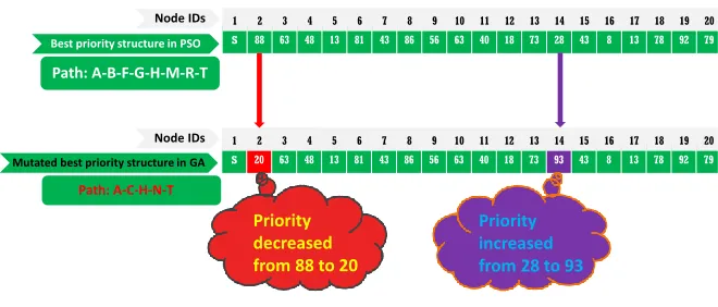
6and7. According to the decoded paths, the PSO (with total path costs of 327) finds a better result or fitness value compared to GA (with total path costs of 349), and thus PSO shares its information with GA. Thereafter, the operators of GA apply to the mixed indi-viduals that GA employs to find as well as or even better result than PSO. For instance, Fig.6shows the two cut-points crossover operator as it applies to the mixed individuals to produce the offspring to reach the global optima and Fig.7depicts the use of mutation operator on the shared information as the priority of node ID increases or decreases. From the produced offspring, the RUBHEA straightforwardly finds the optimal DSP as shown in Fig.5indicated by bold green line with optimal path A-C-H-N-T and its estimated cost is 65+35+20+22=142. It is worth mentioning that the existing algorithms of Ahn et al.10_as

well as Mohemmed et al.29also find feasible results similar to ours for this network model, but our new approach outperforms them in larger network models.

5.4. Encoding method for DSPRP

5.4.1. Population initialization

A B C D E F G H I J K L M N O P Q R S T 50 65 45 43 60 250 27 58 220 20 61 60 ₄₀ 72 71 147 194 220 77 110 150 136 26 61 120 30 230 15 32 40 17 29 30 161 144 130 16 24 89 14 88 30 90 15 32 110 72 50 62 25 32 54 16 88 65 35 20 22 A B C D E F G H I J K L M N O P Q R S T A T

Fig. 5. An example of undirected graph for 20 nodes and 48 edges with optimal path A-C-H-N-T (its cost ⇒ 65+35+20+22=142) showed in bold green line obtained by Ahn et al.10, Mohemmed et al.29, and the proposed RUBHEA with η = 0.05. The results of the GA (path⇒A-E-D-K-J-S-T and its to-tal cost⇒30+90+15+32+110+72 = 349) and the PSO (path ⇒A-B-F-G-H-M-R-T and its total cost ⇒

50+62+25+32+88+54+16 = 327) are indicated by yellow and pink solid lines, respectively.

create an initial population to serve as the starting point for the GA. This initial population is usually created randomly. From empirical studies, over a wide range of function opti-mization problems, a population size of between 20 and 100 is usually recommended10,29_.

On the other hand, the processing time and memory requirement in a PC is increased when the larger population size is used to optimize a problem.

5.4.2. Local search based priority encoding method

S 23 38 68 76 51 33 48 43 55 59 36 67 72 14 46 65 74 86 80

1 2 3 4 5 6 7 8 9 10 11 12 13 14 15 16 17 18 19 20

Path: A-E-D-K-J-S-T

S 88 63 48 13 81 43 86 56 63 40 18 73 28 43 8 13 78 92 79

1 2 3 4 5 6 7 8 9 10 11 12 13 14 15 16 17 18 19 20

Path: A-B-F-G-H-M-R-T

S 23 63 48 13 81 43 86 56 63 40 18 67 72 14 46 65 74 86 80

1 2 3 4 5 6 7 8 9 10 11 12 13 14 15 16 17 18 19 20

Offspring 1 in GA

Path: A-C-H-N-T

S 88 38 68 76 51 33 48 43 55 59 36 73 28 43 8 13 78 92 79

1 2 3 4 5 6 7 8 9 10 11 12 13 14 15 16 17 18 19 20

Path: A-B-F-L-M-R-T

Offspring 2 in GA

Best priority structure in PSO

Best priority structure in GA

Node IDs

Node IDs Node IDs

Node IDs

Fig. 6. Performance of GA operators in RUBHEA: Application of two-cut crossover method to the two optimal paths obtained in the example of undirected graph in Fig.5.

S 88 63 48 13 81 43 86 56 63 40 18 73 28 43 8 13 78 92 79

1 2 3 4 5 6 7 8 9 10 11 12 13 14 15 16 17 18 19 20

Path: A-B-F-G-H-M-R-T

Best priority structure in PSO

Node IDs

Mutated best priority structure in GA S 20 63 48 13 81 43 86 56 63 40 18 73 93 43 8 13 78 92 79

1 2 3 4 5 6 7 8 9 10 11 12 13 14 15 16 17 18 19 20

Path: A-C-H-N-T

Node IDs

Priority decreased from 88 to 20

Priority increased from 28 to 93

Fig. 7. Performance of GA operators in RUBHEA: Application of two-cut crossover method to the two optimal paths obtained in the example of undirected graph in Fig.5.

adja-Ω 56 45 32 65 23 78 1 2 3 4 5 6 7 Node IDs P ri or it y Ω 56 45 ϒ ϒ ϒ ϒ 1 2 3 4 5 6 7 Node IDs P ri or it y ϒ Ω ϒ 32 65 ϒ ϒ 1 2 3 4 5 6 7 Node IDs P ri or it y ϒ ϒ ϒ 32 Ω ϒ 78 1 2 3 4 5 6 7 Node IDs P ri or it y Op timal P ath : 1 -2 -5 -7 Se le ct e d n o d e ID :1 Se le ct e d n o d e ID :2 Se le ct e d n o d e ID :5 Se le ct e d n o d e ID :7 Ω 56 45 32 65 23 78 1 2 3 4 5 6 7 Node IDs P ri or it y Ω 56 45 32 65 23 78 1 2 3 4 5 6 7 Node IDs P ri or it y ϒ Ω 45 32 65 23 78 1 2 3 4 5 6 7 Node IDs P ri or it y ϒ ϒ 45 Ω 65 23 78 1 2 3 4 5 6 7 Node IDs P ri or it y Op timal P ath : 1 -2 -4 -7 Se le ct e d n o d e ID :1 Se le ct e d n o d e ID :2 Se le ct e d n o d e ID :4 Se le ct e d n o d e ID :7

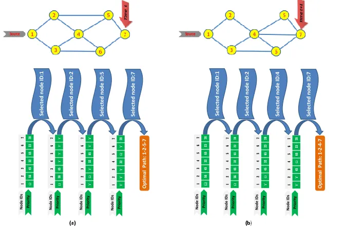
Fig. 8. Two examples of 7 nodes with 10 edges undirected graphs with path representation according to the modified search based priority encoding method. (a) Undirected graph at time t; (b) Undirected graph at time t+1.

cency matrix is maintained in the implementation. This matrix is updated after selection of a node to be included in a path so that the selected node will not be a candidate for future selection. For many combinatorial optimization problems, problem specific encodings are used and these usually yield illegal offspring by a simple one-cut-point crossover opera-tion. Repairing techniques are usually adopted to convert an illegal chromosome to a legal one. Inspired by the use of previous priority based method improvements for DSPRP29_,

we modified priority based encoding by using a local search method. Characterizations of chromosomes and particles have been used to represent valid paths. A gene in a chro-mosome is characterized by two factors: the position of the gene within the structure of chromosomelocus, i.e., the position of the gene located within the structure of chromo-some, andallele, i. e., the value the gene takes. In RUBHEA encoding method, the position of a gene is used to represent path among candidate and a path can be uniquely determined from this encoding. Furthermore, a particle in the search space is also characterized by two factors: itsposition, i. e., represents the Node ID in a structure of particle, and thevelocity, i. e., represents the distance to be travelled by this particle from its current position.

3 and so is entered into the path. The possible nodes next to node 2 are nodes 1, 4, and 5 but the first must be removed and its priority set to any negative numberΥbecause it is the source and thus already in the path. Thus, node 5 has the largest priority value and is placed into the path. The formation of the set of nodes available for the next position results in the selection of node 7 to deliver the valid path (1-2-5-7). Fig.8 (b) shows the modified search with priority based method employed in the undirected connection network where the nodes changed their position in the environment.

6. Results and Discussions

To benchmark the performance of RUBHEA, we compared it with GA-based and PSO-based dynamic shortest-path routing algorithms as implemented by Ahn et al.10_{, and}

Mo-hemmed et al.29, respectively. In addition, we investigated the performance of RUBHEA with various population intersection percentages; this is further discussed when compar-isons are made with recently published hybrid algorithms12,6. Following the established practice in the literature10,24,29_{, randomly generated networks with different number of}

nodes, varying numbers of edges and randomly assigned link costs were used to assess the performance of the algorithms in finding the DSP in continuously changing network models. In addition, non-parametric tests have been performed to statistically show that our approach is better than its competitors proposed by Ahn et al.10, Juang12, Marinakis et al.6_{, and Mohemmed et al.}29_.

6.1. Multiple comparisons without statistical tests

In this subsection, we have showed the impact of the individuals of GA and PSO in RUB-HEA followed bythe performance comparison of RUBRUB-HEA for random network topolo-gies based on both GA (e.g., Ahn et al.10_{) and PSO (e.g.,Mohemmed et al.}29_{) as well as}

hybrid of GA and PSO algorithms (e.g., Juang (HGAPSO)12 and Marinakis et al. (Hyb-GENPSO)6).

6.1.1. Used parameters

In the GA implementation, two point uniform crossover was employed withpc = 0.8and pm= 0.01to evolve the initial population. The parent selection was via the roulette wheel

selection method and the fitness values were ascertained in each of the GA iterations. In the PSO implementation, the particle positions and velocities were initialized with random real numbers and the learning factorsc1andc2were set to 2. To create dynamically changing

network models, the network simulator Sinalgo51 _{was used. We randomly generated six}

used, one being the achievement of the optimal fitness value and the other the reaching of a previously set iteration limit.

6.1.2. Impact of the individuals of GA and PSO in RUBHEA

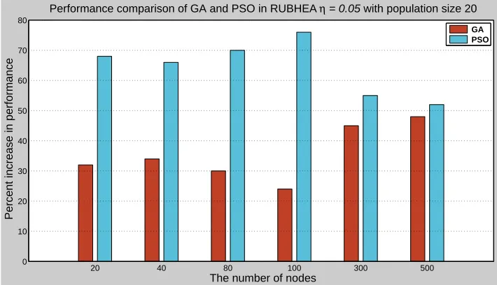
In RUBHEA, strong PSO particles replaced weak chromosomes in the population of the GA or vice versa with the decision iteratively based on the sub-population fitness values evaluated until the algorithm terminated. Fig. 9shows the impact of the GA individuals and PSO particles in RUBHEA withη= 0.05in the achievement of the best fitness value. The lowest population intersection percentage was chosen to analyze and understand the impact of the populations in RUBHEA because this provided the best results with the least distortion of the populations. From the figure, PSO substantially out performs the GA in small network models but advantage is modest for very large networks. For instance, when the network contains 20 nodes, the particles in PSO is reaching the global optimum 68% of the time compared to just 32% with the GA chromosomes, i.e., PSO performs68/32≈2.1 times better. This kind of performance improvement of PSO also confirms the claims of Mohemmed et al.29_{as well as Marinakis et al.}6_{. Mohemmed et al.}29_{where a comparison}

of PSO-based search algorithm and a GA for solving the DSPRP was proposed and the authors claimed that the PSO-based algorithm was superior to that using GA for finding DSP in dynamically changed networks. Marinakis et al.6 proposed a hybrid of GA and PSO for the vehicle routing problem and claimed that by the effect of PSO the use of an intermediate phase between two generations gave more efficient individuals and would improve the effectiveness of their HybGENPSO algorithm. However, it should be borne in mind that the common test networks such as the Chinese National Network (CHNNET) and ARPANET contain relatively small numbers of nodes (15 and 20, respectively)52. Henceforth, RUBHEA will deliver substantial benefits for practical network design based on the superior PSO performance and will still perform well for very large networks.

6.1.3. Route failure ratio performance for RUBHEA and others

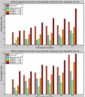
The route optimality was considered since this is the most common and widely-used def-inition for investigating the performance of algorithms. The defdef-inition of route optimality (or success rate) is the mean percentage of times that the algorithm finds the global op-timum (shortest-path) over a large number of runs. Here, use is made of the route failure ratio, which is the fraction of the runs which result in non-optimal computed routes. Since the performance of RUBHEA will vary with the population intersection valueη, three dif-ferent values ofηwere employed, i.e.,η={0.05,0.50,1.00}. Fig.10illustrates the route failure ratio performance for various algorithms with different network models. The algo-rithm of Mohemmed et al.29performed the best with population size 20 and 20 nodes. A network model having 100 nodes and a population size of 20, RUBHEA withη = 0.05 delivered a route failure ratio of just 0.09 (implying a route optimality of 91%) and the algorithm of Mohemmed et al.29 _{produced 0.17 (i.e., a route optimality of 83%) which}

The number of nodes

Percent increase in performance

Performance comparison of GA and PSO in RUBHEA η = 0.05 with population size 20

20 40 80 100 300 500

0 10 20 30 40 50 60 70 80

GA PSO

Fig. 9. Impact of the individuals of GA and PSO in RUBHEAη= 5%to achieve the best fitness value.

Ahn et al.10_{resulted in route failure ratios of more than 0.30 (i.e., a route optimality up to}

70%). With this simple statistic, RUBHEA withη = 0.05is reducing the failure rate by up

to1−0.09/0.17 = 0.47or 47% as compared to the algorithm of Mohemmed et al.29_or

RUBHEA withη= 0.50as well as up to1−0.09/0.30 = 0.70or 70% as compared to the algorithm of Ahn et al.10or RUBHEA withη= 1.00, i.e., on the average up to 58.50%.

The algorithm of Ahn et al.10_{lacked behind both Mohemmed et al.}29_{and RUBHEA}

withη = 0.50in employed all network models. With the increasing of population size and/or nodes RUBHEA withη = 0.50showed the upper hand over Mohemmed et al.29_,

RUBHEA withη= 0.50, Ahn et al.10, and RUBHEA withη = 1.00; i.e., RUBHEA with

η = 0.05 provided the highest performance. Intrusively speaking, RUBHEA withη = 0.05gave the best performance and this decreased with increased population intersection percentage. Furthermore, the quality of solution increased when a higher population size was employed as shown in Fig. 10(b) because the increase population provided more chances for evolution. For instance, determined route failure ratio of RUBHEA withη = 0.05for the case study of VI was 0.19 with a population size of 20 but decreased to 0.13

or1−0.13/0.19 = 31.6%when the population size was 40.

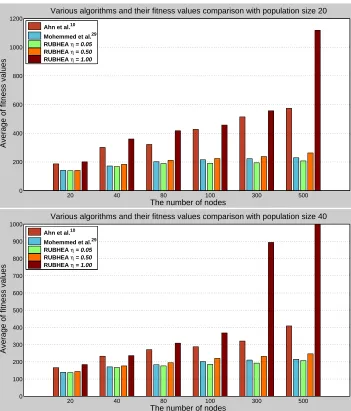
6.1.4. Average fitness function values for RUBHEA and others

The number of nodes

Route failure ratio

Different algorithms and their route optimality comparison with population size 20

20 40 80 100 300 500

0 0.1 0.2 0.3 0.4 0.5 0.6 0.7

Ahn et al.10

Mohemmed et al.29

RUBHEA η = 0.05

RUBHEA η = 0.50

RUBHEA η = 1.00

The number of nodes

Route failure ratio

Different algorithms and their route optimality comparison with population size 40

20 40 80 100 300 500

0 0.1 0.2 0.3 0.4

Ahn et al.10

Mohemmed et al.29

RUBHEA η = 0.05

RUBHEA η = 0.50

RUBHEA η = 1.00

Fig. 10. Comparison of the route optimality with various algorithms for six different network models.

ered. Increased population intersection again decreased the performance but RUBHEA withη = 0.50still delivered similar results to the algorithm of Mohemmed et al.29 _and

much better outcomes than the algorithm of Ahn et al.10. Increasing the intersection to

The number of nodes

Average of fitness values

Various algorithms and their fitness values comparison with population size 20

20 40 80 100 300 500

0 200 400 600 800 1000 1200

Ahn et al.10

Mohemmed et al.29

RUBHEA η = 0.05

RUBHEA η = 0.50

RUBHEA η = 1.00

The number of nodes

Average of fitness values

Various algorithms and their fitness values comparison with population size 40

20 40 80 100 300 500

0 100 200 300 400 500 600 700 800 900 1000

Ahn et al.10

Mohemmed et al.29

RUBHEA η = 0.05

RUBHEA η = 0.50

RUBHEA η = 1.00

Fig. 11. Comparison of the estimated fitness values with various algorithms for six different network models.

withη= 0.05using population sizes of 20 and 40, showing that the algorithm works well with a small population size. As a result, the fitness function in RUBHEA optimizes the dynamic shortest paths effectively as compared to other fitness functions shown in Fig11.

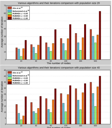
Fig12depicts the average number of iterations required to achieve the feasible solution, showing that RUBHEA withη= 0.05found the optimum route with the smallest number of iterations. For example, the algorithm of Mohemmed et al.29required 9 iterations for 20 nodes using population size 40 and for the same the algorithm of Ahn et al.10_{took some}

The number of nodes

Average number of iteration

Various algorithms and their iterations comparison with population size 20

20 40 80 100 300 500

0 10 20 30 40 50 60 70

Ahn et al.10

Mohemmed et al.29

RUBHEA η = 0.05

RUBHEA η = 0.50

RUBHEA η = 1.00

The number of nodes

Average number of iteration

Various algorithms and their iterations comparison with population size 40

20 40 80 100 300 500

0 5 10 15 20 25 30 35 40 45

Ahn et al.10

Mohemmed et al.29

RUBHEA η = 0.05

RUBHEA η = 0.50

RUBHEA η = 1.00

Fig. 12. Comparison of the average number of iterations with various algorithms for six different network models.

4 iterations, i.e., it has 1−4/9 ≈ 56% and1−4/16 = 75%better performance over Mohemmed et al.29_{and Ahn et al.}10_{, respectively. As one would expect, employing the}

algorithms with the higher population size gave better results as shown in Fig.12(b) but this caused a higher memory requirement in the computer.

The number of nodes

Average of Fitness Values

Different hybrid algorithms and their fitness values comparison with population size 20

20 40 80 100 300 500

0 50 100 150 200 250

RUBHEA η = 0.05

HGAPSO12

HybGENPSO6

Fig. 13. Comparison of the average number of estimated fitness values for three hybrid algorithms.

of Mohemmed et al.29.

6.1.5. Comparing RUBHEA with other hybrid algorithms

The main conclusion from the tests described in the previous section is that the proposed method gives effective results as long asηis small. To further understand and analyze the performance and the capability of the RUBHEA approach here, it has been compared to recently used hybrid algorithms for recurrent network design (HGAPSO12) and vehicle routing (HybGENPSO6_{). In both the HGAPSO}12_{and HybGENPSO}6_{algorithms, GA and}

PSO work with the same population. In the HGAPSO12, the best 50% of individuals are evaluated and enhanced by using the operators of GA and PSO. In HybGENPSO6_{, the}

operators of GA and PSO are, respectively, applied to the all individuals to produce the new generation. Fig.13depicts the average number of estimated fitness values. The al-gorithm of HybGENPSO6_{is slightly better than that of HGAPSO}12_{based on finding the}

low average number of fitness values in all network models presented hereby. However, the proposed RUBHEA withη = 0.05finds the lowest average number of estimated fit-ness values in all network models. Although the existing hybrid algorithms give feasible results similar to ours for small network models, our new approach outperforms them in larger network models. Fig.14shows that the algorithm of HGAPSO12_{is better than that}

of HybGENPSO6in terms of the average number of iterations. It also demonstrates that the convergence rate of the RUBHEA withη = 5%is much better than HybGENPSO6

The number of nodes

Average number of iterations

Different hybrid algorithms and their iterations comparison with population size 20

20 40 80 100 300 500

0 5 10 15 20 25 30

RUBHEA η = 0.05

HGAPSO12

HybGENPSO6

Fig. 14. Comparison of the average number of iterations to get the feasible solution for three hybrid algorithms.

6.2. Multiple comparisons with statistical tests

Multiple comparisons with a control algorithm have commonly been used to statistically show that one approach is better than its competitors in areas related to computer science. The main idea of using the non-parametric tests54_{is that they can deal with probabilistic}

and non-probabilistic methods without any limitation. In this subsection, non-parametric test results are presented and examined for comparing the proposed algorithms with the rest of algorithms. We have performed tests adequate to multiple comparisons together with a set of post-hoc procedures to compare a control algorithm with other algorithms (1×N

comparisons) or to perform all possible pairwise comparisons (N×Ncomparisons). As we know, in conducting a test of significance or hypothesis test there are two im-portant numbers namelyp-value of the test statistic and the level of significanceα. Both

p-value andαcould be easily confused because they are both numbers between zero and one, and are in fact probabilities. The number αtells us how extreme observed results must be in order to reject the null hypothesis of a significance test. Thep-value of the test statistic is a way of saying how extreme that statistic is for our sample data. The smaller thep-value, the more unlikely the observed sample. In statistical significance testing, the

6.2.1. Various nonparametric tests

Friedman test56 _{and its derivatives (e.g., Iman-Davenport test}57_{) are usually referred as}

one of the most important non-parametric tests for multiple comparisons. First of all, we have performed the Friedman test56_{. A usable characteristics of this test is that it ranks the}

algorithms from the best performing to the poorest one. However, it can only inform the re-searcher about the presence of differences among all samples of results compared. We have also performed two more alternatives the Friedman Aligned Ranks58and the Quade test59, which differ in the way of computing the rankings and may lead to better results depend-ing on the features of the experimental study considered. After the null-hypotheses have been rejected, we have proceeded with the post-hoc procedures to find the particular pairs of algorithms which produce differences. The post-hoc procedures comprise Bonferroni-Dunn’s60, Holm’s61, Hochberg’s62, Hommel’s63,64, Holland’s65, Rom’s66, Finner’s67, and Li’s68_{, procedures in the case of1×N comparisons, and Nemenyi’s}69_{, Shaffer’s}70_{, and}

Bergmann-Hommel’s71procedures in the case of N×N comparisons. The Bonferroni-Dunn’s procedure60leads to the statement that the performance of two algorithms is sig-nificantly different if the corresponding average of rankings is at least as great as its critical difference. More powerful is Holms procedure61which checks sequentially hypotheses or-dered according to their p-values from the lowest to the highest. All hypotheses for which p-value is less than the significance levelαdivided by the number of algorithms minus the number of a successive step are rejected. All hypotheses with greater p-values are sup-ported. Holland’s65 and Finner’s67procedures, also adjust the value ofαin a step-down manner as Holm’s step down method61does. The Hochberg’s procedure62operates in the opposite direction to the former, comparing the largestp-value withα, the next largest with

α/2, and so forth until it encounters a hypothesis it can reject. Rom66devised a modifi-cation to Hochberg’s step-up procedure62 _{to increase its power. In turn, Li}68_{proposed a}

two-step rejection procedure.

6.2.2. Tools used for nonparametric tests

Statistical analysis of the results of experiments was performed using the available soft-warea and the open source JAVA program calculates multiple comparison procedures: Friedman56_{, Iman et al.}57_{, Bonferroni et al.}60 _{, Holm}61_{, Hochberg}62_{, Holland}65_{, Rom}66_,

Finner67, Li68, Shaffer70, and Bergamnn et al.71tests as well as adjustedp-values. When all possible pairwise comparisons need to be performed, the easiest is the Ne-menyi’s procedure69. It assumes that the value of the significance levelαis adjusted in a single step by dividing it merely by the number of comparisons performed. It is a very sim-ple way but has little power. The Shaffer’s static routine70_{, in turn, follows the Holm’s step}

down method61. At a given stage, it rejects a hypothesis if thep-value is less thanαdivided by the maximum number of hypotheses which can be true given that all previous hypothe-ses are false. The Bergmann et al.’s71scheme is characterized by the best performance, but it is also the most sophisticated and therefore difficult to understand and computationally