http://wrap.warwick.ac.uk/
Original citation:Mengus, Eric and Pancrazi, Roberto (2015) The inequality accelerator. Working Paper. Coventry: University of Warwick. Department of Economics. Warwick economics research papers series (WERPS) (1067). (Unpublished)
Permanent WRAP url:
http://wrap.warwick.ac.uk/73200
Copyright and reuse:
The Warwick Research Archive Portal (WRAP) makes this work of researchers of the University of Warwick available open access under the following conditions. Copyright © and all moral rights to the version of the paper presented here belong to the individual author(s) and/or other copyright owners. To the extent reasonable and practicable the material made available in WRAP has been checked for eligibility before being made available.
Copies of full items can be used for personal research or study, educational, or not-for-profit purposes without prior permission or charge. Provided that the authors, title and full bibliographic details are credited, a hyperlink and/or URL is given for the original metadata page and the content is not changed in any way.
A note on versions:
The version presented here is a working paper or pre-print that may be later published elsewhere. If a published version is known of, the above WRAP url will contain details on finding it.
Warwick Economics Research Paper Series
The Inequality Accelerator
Eric Mengus & Roberto Pancrazi
The Inequality Accelerator
∗
Eric Mengus
Roberto Pancrazi
September 15, 2015
PRELIMINARY
Abstract
We show that the transition from an economy characterized by idiosyncratic income shocks and incomplete markets `a laAiyagari(1994) to markets where state-contingent assets are available but costly (in order to purchase a state-contingent asset, households have to pay a fixed participation cost) leads to a large increase of wealth inequality. Using a standard calibration our model can match a Gini of 0.93 close to the level of wealth inequality observed in the US. In addition, under this level of participation costs, wealth inequality is particularly sensitive to income inequality. We label this phenomenon as the Inequality Accelerator. We demonstrate how costly access to contingent asset-markets generates these effects. The key insight stems from the non-monotonic relationship between wealth and desired degree of insurance, in an economy with participation costs. Poor borrowing constrained households remain uninsured, middle-class households are almost perfectly insured, while rich households decide to self-insure by purchasing risk-free assets. This feature of households’ risk management has crucial effects in asset prices, wealth inequality, and social mobility.
JEL codes: D31, E21, G11.
Keywords: Wealth Inequality, Participation costs, Insurance.
∗Mengus: HEC Paris. Email: [email protected]. Pancrazi: University of Warwick, department of
1
Introduction
A widely adopted assumption in macroeconomic models is that households can
per-fectly participate in asset markets. Then, in presence of idiosyncratic risk, complete and
freely-accessible markets imply a non-existing endogenous evolution of wealth inequality,
since agents with different income realizations optimally decide to provide insurance to
each other. We refer to this outcome as the perfect-insurance equilibrium. This setting
is obviously not suited for analyzing inequality. The polar opposite case is the
incom-plete market assumption, under which households do not have access to state-contingent
assets, simply because those assets do not exist (Bewley, 1980; Deaton, 1991; Aiyagari,
1994; Krusell and Smith, 1998). This setting generates a self-insurance equilibrium, in
which agents buy or sell risk-free bonds to intertemporally smooth their idiosyncratic
shocks. Interestingly, the incomplete market model suffers from two caveats. First, from
a theoretical point of view, the incomplete market model is not able to generate the
large wealth inequality as observed in the data, as summarized inQuadrini and Rios-Rull
(2014), unless it includes unrealistic income processes, as inCastaneda et al.(2003).1
Sec-ond, from an empirical point of view, conducting an empirical analysis on labor income
risk and insurance, Guvenen and Smith (2014) find that the amount of uninsurable
in-come risk perceived by individuals is substantially smaller than what it is typical assumed
in incomplete market models.
In this paper we propose a solution for these caveats. We consider an intermediate case
between the two polar cases, i.e. the perfect-insurance equilibrium and theself-insurance
equilibrium. In our setting markets that potentially provide full insurance do exist, but
it is costly to access to them. In an otherwise standard general equilibrium economy, we
introduce costs for participating in contingent asset markets. Specifically, in our
frame-work households have to payqa+κto purchasea contingent bonds, whereq denotes the price of the asset, and κ denotes the additional fixed participation cost.2 Consequently, households face a trade-off between paying the participation cost and enjoying the gain
of consumption smoothing. For a large set of values of the participation cost κ, the economy is, then, characterized by a partial-insurance equilibrium, where only a fraction
of the population is insured. In the first section of the paper we provide the intuition
1As commented in Quadrini and Rios-Rull (2014), the persistence of income process in Castaneda
et al.(2003) is “engineered” to be able to replicate the observed wealth inequality.
2The idea that consumption smoothing is costly underpins our approach: being active in financial
behind this result by analyzing a simple insurance model similar to the one in Kimball
(1990b); the necessary condition for the existence of a partial-insurance equilibrium is
assuming that agents’ utility features decreasing absolute prudence (or equivalently a
positive forth derivative). In this case, the precautionary-saving premium asked by the
agent is decreasing in wealth. Notice that, as discussed in Kimball (1990a), commonly
used parameterizations of the utility function, such as the constant relative risk aversion
utility, displays decreasing absolute prudence.
In the more general economy we demonstrate that our setting leads to novel findings
about the relationship between degree of insurance, income risk, and wealth inequality.
Specifically, when participation costs reduce from a arbitrary large value, such that the
economy is equivalent to a self-insurance equilibrium, to intermediate values, such that
the economy turns into apartial-insurance equilibrium, wealth inequality can dramatically
increase. With intermediate value of participation costs our model can predict a level of
wealth inequality similar to the one observed in the U.S. data (Gini index equal to 0.93).
Notice that when we increase the participation cost such that our economy behaves
as an incomplete market model as in Aiyagari (1994), the wealth Gini index is much
lower and equal to 0.12. Hence, our model can predict a large wealth inequality starting
with a much less disperse income process than in Castaneda et al. (2003).3 Our result,
then, links the increased innovation in the financial sector in the last three decades, as
documented by Lerner (2002) to the increased wealth inequality in the same time span,
as reported by Saez and Zucman(2014). Also, when participation costs reduced further,
the economy transits to a perfect-insurance equilibrium, and wealth inequality reduces
to zero, thus leading to an interesting non-monotone relationship between participation
costs and wealth inequality.
Additionally, the partial-insurance equilibrium equilibrium leads to a non-trivial
rela-tionship between income risk and wealth inequality. In fact, in an economy characterized
by intermediate levels of participation costs, a certain (small) degree of income inequality
triggers a very large amplification from income inequality to wealth inequality, driven by
the non-monotone willingness to insure across the wealth distribution and its implications
on asset prices. We label this phenomenon as the Inequality Accelerator. With a
numer-ical example, we find that a small increase of the exogenous income inequality in the
participation-cost model leads to a very large change of the resulting wealth inequality.
Crucially, however, the same change in income dispersion implies a vary small increase of
the wealth inequality in the incomplete market model.
How can wealth inequality increase from a reduction of participation costs to financial
3For example, income dispersion, measured as Gini index on income, in our model is 0.097, whereas
markets? The answer for this question stems from the non-monotone relationship between
households’ insurance desire and their wealth generated by the participation cost model.
Hence, the first contribution of the paper is to closely characterize households’ decision
about participating in asset markets. Specifically, we consider a standard neoclassical
model with idiosyncratic shocks as in Aiyagari (1994). We assume that households can
purchase two type of assets: a state contingent asset, which can be purchased only by
paying a fixed participation cost, and a risk-free asset. First, agents decide whether
they want to participate in the financial markets, and, then, they decide against which
states they are willing to buy insurance. We demonstrate that this discrete choice about
financial market participation can be solved with standard recursive methods by using
value functions. Also, we prove that households decide to participate in a contingent
market as long as its participation cost is lower than a certain threshold value. Intuitively,
the threshold depends positively on the households’ gains of insurance, and it depends
non-monotonically on households’ wealth, for a large variety of utility functions. As
a result, the partial-insurance equilibrium is characterized by a set of poor households
that are not able to obtain any insurance, by a set of middle-class household that actively
participate to the contingent asset market and, hence, are fully insured, and, interestingly,
by a set of rich households that prefer to self insure by accumulating a large stock of the
risk-free assets. In the empirical section of the paper we directly test the non-monotonic
distribution of insurance across wealth, using the Bank of Italy Survey of Households’
Income and Wealth (SHIW) data.
The second contribution of the paper is to explore the consequences of the
non-monotone relationship between insurance and wealth for inequality, partial insurance,
and welfare. Specifically, we demonstrate that the partial-insurance equilibrium features
two forces that lead to a skewed wealth distribution. First, perfectly insured middle-class
households do not accumulate more assets and, as the risk-less interest rate is lower than
in the complete market model, they even progressively consume their wealth. Second,
self-insured richer households benefit from real interest rates that are higher than in the
incomplete market model and they accumulate more wealth in comparison with the
stan-dard Aiyagari model. These two forces reinforce the social disparity from the rich that
accumulate wealth and the rest of the population. As a result, the upper tail of the
wealth distribution thickens in presence of intermediate levels of participation costs.
Participation costs lead some households to choose to be perfectly insured and some
other households to choose to be only self-insured. Hence, the fraction of population that
is perfectly insured is a function of the level of participation costs. We can then draw a
similarity between the degree of partial insurance discussed inGuvenen and Smith(2014).
a fraction of their income, whereas in our setting partial insurance is on the extensive
margin - agents can be insured or not. Using different calibrations of the model, we show
that degrees of partial insurance above and below the one estimated by Guvenen and
Smith(2014), around 45 percent, can lead to the realistically observed wealth inequality
in presence of participation costs.
In terms of welfare, we find that insurance decisions are usually not constrained
effi-cient, because of a pecuniary externality arising through factor prices, similarly toDavila
et al. (2012). In addition, we also find that a similar externality affects insurance
deci-sions: competitive-market insurance participation may exceed its social-planner level in
the partial-insurance equilibrium, because of the distortions in asset prices and wages.
This happens due to the resulting large level of wealth inequality, which makes more
capi-tal desirable so as to redistribute resources through higher wages. Interestingly, this result
reverts with higher participation costs and lower wealth inequality, for which
competitive-market insurance participation is lower than its social-planner level.
Related literature. In addition to the papers that we have already mentioned, our
work expands on several bodies of the literature.
Among the empirical studies conducted on lack of insurance and consumption
smooth-ing as Townsend (1994) andMace (1991), our work bears similarity to that of Cochrane
(1991), and, more recently,Grande and Ventura(2002), who study households’ insurance
against different types of risk. They show that households are well insured against
cer-tain types of risks, such as health problems, but not against other types of risks, such as
unemployment (especially involuntary job loss) (see alsoBlundell et al., 2008).
Our paper shares similarities with the literature on welfare. Since our focus is on
par-ticipation costs, our approach resemble that ofTownsend and Ueda (2010), who consider
the welfare effect of financial liberalization, which leads to better consumption insurance.
It is also related to the literature on the constrained Pareto optimality of idiosyncratic
shock models asCarvajal and Polemarchakis(2011) or Davila et al.(2012) among others,
or on the welfare cost of incomplete markets (seeLevine and Zame, 2002). Here, we find
sizable effects of incomplete markets on risk-sharing as the agents that we consider are
sufficiently impatient.
Our work also amplifies on the literature linking models of incomplete insurance with
empirical evidence as in Krueger and Perri (2005, 2006) or Kaplan and Violante (2010),
who assess the degree of insurance beyond self-insurance. In our setting the participation
cost modifies the link between income and consumption inequality, through the resulting
non-monotone degree of insurance across wealth. Hence, trends in one of these variables
(2012) and Aguiar and Bils (2015).
Finally, our work links to the literature in finance on limited participation as in
Luttmer (1999), Vissing-Jorgensen (2002) and more recently in Paiella (2007),
Guve-nen (2009) orAttanasio and Paiella (2011) among others. In these models, stock market
is open only in a subset of periods. Also, even when economists focus on limited asset
trading,4 they generally do not consider frictions related to asset market participation in
their models.
The rest of the paper is organized as follows: in Section2we present a simple insurance
model in order to provide conditions and intuitions for households’ insurance decision.
In Section 3 we describe the general economic environment. Section 4 characterizes the
individual asset market participation decisions. Section5presents the results about social
mobility, wealth inequality, and welfare. In Section 6 we empirically test the presence
of the non-monotone insurance behavior across wealth using the Bank of Italy Survey
of Households’ Income and Wealth (SHIW) data. Section 7 discusses a set of further
extensions. Finally, Section 8provides concluding remarks.
2
A Simple Insurance Model
In order to gain some intuition about households’ individual contingent-market
par-ticipation choice, we first analyze a simple two-period and two-state insurance model.
Our model is similar to the one proposed in Kimball (1990a) and in Kimball (1990b), in
which we include a fix cost to state contingent asset market participation
The economy lasts two periods, t = 0,1. The household is endowed with a level of wealthW in both periods. In periodt= 1 the household might face an exogenous loss of wealth, −L≥0, which occurs with probabilityp. With probability 1−p, the household receives a positive shockpL/(1−p) so that the expected loss is 0. The indicator variable 1Ldescribes the realization of the state of nature. Let define asfeasiblethe levels of wealth
such thatW > L, to assure that consumption is positive in every period and in every state. The household maximizes the following expected utility function: E0(u(c0) +u(c1)). For
simplicity, we assume that there is no discounting.
We introduce an endogenous decision of participating in the insurance market. The
agent has access to state contingent assets. At time t = 0, the agent can acquire α
units of a state-contingent asset at unit price qα that repay a unit of consumption good 4This can happen because of lack of commitment (Thomas and Worrall, 1988;Kocherlakota,1996),
at time t = 1 only if the loss in wealth occurs, i.e. if 1L = 1, and β units of a state-contingent asset at unit price qβ that repay a unit of consumption good at time t = 1 only if the loss in wealth does not occur, i.e. if 1L = 0. Importantly, in order to have
access to the state contingent asset, the agent needs to pay a fixed costκ. The household is not necessarily willing to pay the fixed cost and, hence, we define δ(W, κ) as a choice variable that denotes the contingent asset market participation, given a level of wealth
and a participation cost: if the household pays the cost and purchases contingent assets,
δ(W, κ) equals 1. Otherwise, it equals 0.
Conditional on participation, δ(W, κ) = 1, the budget constraints are:
c0+qαα+qββ+κ=W
c1 =W + 1L(α−L) + (1−1L)(β+pL/(1−p)).
Without loss of generality, we assume the prices of the contingent asset are actuarially
fair, (qα =pandqβ = 1−p). In this case, the optimal amount of insurance is: α=L−κ/2 and β =−κ/2−pL/(1−p), and agent’s expected utility is:
VP(W, κ) = 2u(W −κ/2),
where the superscript P denotes the expected of utility of an agent that participates to the insurance market.
Conditional on no-participation, δ(W, κ) = 0, the two periods budget constraints are:
c0 =W
c1 =W −1LL+ (1−1L)pL/(1−p). The expected utility of the agent is:
VN(W) =u(W) +
(1−p)u
W + pL 1−p
+pu(W −L)
,
where the superscriptN indicates the utility of an agent with no access to the insurance market. Let P(κ) be the set of wealth levels for which participation in the insurance market is optimal for a given participation cost κ. Formally:
Definition 1. (Participation Set). For a given participation cost κ, for any wealth level inP(κ) insurance market participation is optimal, that is:
P(κ) =W ∈(L,∞) :VP(W, κ)> VN(W) .
Let define the gain of insurance as G(W, κ) = 12 VP(W, κ)−VN(W). It can be rewritten as:
G(W, κ) =uW − κ
2
− 1
2u(W)− 1−p
2 u
W + pL 1−p
− p
Proposition 1. (Insurance Incentives without cost) Letu(x) be a three-times continuous and differentiable utility function, such that u0(x)>0, u00(x)<0, and satisfies the Inada conditions: lim
x→∞u
0(x) = 0, and lim
x→0u
0(x) =∞. Then, for any feasible level of wealth, i.e.
∀W > L:
1. G(W,0)>0 ;
2. lim
W→∞G(W,0) = 0.
3. If u000 >0 then ∂G∂W(W,0) <0 .
See Appendix C.1 for the proof.
Proposition 1shows that, absent any cost,κ= 0, the (strictly) concavity of the utility function guarantees a (strictly) positive benefit from insurance. If the utility function has
a positive third derivative, its marginal utility is convex and, therefore, displaysprudence,
as defined in Kimball (1990b), and a decreasing absolute risk aversion. In this case, the
gains from insurance G(W,0) are decreasing with respect to wealth. As discussed in
Kimball (1990a), prudence measures the strength of the precautionary saving motive,
which induces individuals to prepare and forearm themselves against uncertainty they
cannot avoid- in contrast to risk aversion, which is how much agents dislike uncertainty
and want to avoid it.
We now consider the economy with participation costs.
Proposition 2. (Insurance Incentive with cost) Let u(x)be a four-times continuous and differentiable utility function, such that u0(x)>0, u00(x)<0, u000(x)>0, u0000(x)<0, and satisfies the Inada conditions: lim
x→∞u
0(x) = 0, and lim
x→0u
0(x) =∞. Then, for any feasible
level of wealth, i.e. ∀W > L, and for any feasible level of cost, i.e. κ <2L:
1. (Existence of Thresholds). Let ˆκ < 2L be the solution of G(L,κˆ) = 0. Then,
∀κ <ˆκ, ∃! W(κ)> L: W ∈P(κ) ⇐⇒ L < W < W(κ).
2. (Comparative static of participation set)
• Participation set coincides with all feasible wealth levels whenκ = 0, that is:
P(0) ={W :W > L}.
• Participation set is shrinking in participation cost, that is for all κ1 < κ2, if W ∈P(κ2) then W ∈P(κ1); hence, P(κ2)⊂P(κ1).
• Participation set is empty for any participation cost greater than κˆ, that is:
See Appendix C.2 for the proof.
This proposition explains a crucial characteristic of the insurance market. When
ac-cessing to the insurance market is costly, the agent endogenously decides whether to
par-ticipate in that state-contingent asset market depending on the level of its wealth. When
wealth level is large enough,W > W(κ), the agent is better off by not-participating in the insurance market since the cost of paying the fix cost is larger than the expected benefit
of reducing the loss in case of occurrence of the negative shock. For those wealth levels,
in fact,G(W, κ)<0. Also, notice that the participation set varies with the participation cost. When the cost tends to zero, the participation set corresponds to the entire feasible
wealth domain. On the contrary, the participation region disappears when the cost is
larger than a certain threshold ˆκ. In this case entering in the insurance market is either infeasible or not beneficial. The necessary condition for the existence of the threshold
wealth level is a strictly negative forth derivative of the instantaneous utility function.
This condition is equivalent to assume a utility characterized by decreasing absolute
pru-dence. As described byKimball (1990a), which relates this assumption to precautionary
saving behavior, approximate constancy for the wealth elasticity of risk-taking is enough
to guarantee decreasing absolute prudence. Also, commonly used parameterizations of
the utility function, such as the constant relative risk aversion utility, displays decreasing
absolute prudence.
3
Model
In this section we describe the general economic environment. We consider an infinite
horizon production economy populated by a continuum of mass 1 ofex ante homogenous
households. This model follows closely Aiyagari (1994) except for two dimensions: we
introduce securities contingent to idiosyncratic states and we simultaneously introduce
fixed participation costs for each contingent market. Time is discrete and indexed by
t∈ {0,1, ...}.
Uncertainty and preferences. Each Household chooses consumption so as to
max-imize the following utility: U =EP
ytβtπ(yt)u(c(yt)), where β ∈ (0,1) is the discount
factor, c(yt) denotes consumption at date t, and u is a strictly increasing and concave function that satisfies limc→0u0(c) =−∞ and limc→∞u0(c) = 0. Without loss of
general-ity, u is twice differentiable.
Households inelastically provide labor. At every period they receive a stochastic labor
constant wage rate.
We assume that yt follows a Markov process, which takes values in Y = {y1, ...yN} and that π(yj|yk) is the associated transition probability from state j to state k. We denote byyt the history of the realizations of the shock,yt={y
0, y1, ..., yt}, and by Π(yk) the fraction of households in state k.
Remark. Note that since there is no aggregate uncertainty here the fraction of households
in each state is constant.5
Asset structure. To smooth consumption, households may trade a set of different
assets. First, they can purchase non-contingent bonds. Each of these bonds yields,
unconditionally, one unit of goods next period. We denote by B(yt) household’s position in the risk-free assets and by qf its price. Besides, as in Aiyagari (1994), we impose that this position is bounded below: B(yt) ≥ −B where B ≥ 0 is finite.6 Second, households can trade a set of state-contingent assets. In state ym, each of these assets pays contingently to the realization of yk next period: it pays 1 when y = yk and 0 otherwise. We denote byq(k, m) the price of this asset and bya(k, yt) the corresponding holdings of a household with history of shocks yt. Note that in our notation contingent asset holding depends on the current state m through the history of shock yt.
The novelty we introduce in this paper is that purchasing those assets requires paying
a fixed fee, κ. Hence, in order to hold a(k, yt) units of any contingent assets household has to payq(k, m)a(k, yt) +κ. Here, for simplicity, we assume that if the agent pays the participation cost she can purchase or sell the preferred quantity of any state contingent
assets. We assume that κ is a pure waste.7
The presence of the fixed cost implies that the household needs to take a discrete
decision about whether to participate in the contingent asset market. We denote by
δ(yt) ∈ {0,1} the corresponding decision variable, with the following meaning: when
δ(yt) = 1, household with history yt decides to enter in the state-contingent assets and when δ(yt) = 0, she does not.
5This assumption can be relaxed; to solve the corresponding model with aggregate uncertainty,Krusell
and Smith (1998)’ methods are needed. Yet, this is beyond the scope of this paper, which focuses on idiosyncratic shocks only.
6We do not provide further foundations for that constraint. It can be exogenous debt limits as in
Bewley(1980), natural debt limits as inAiyagari(1994) or endogenous borrowing constraints as inZhang
(1997) orAbraham and Carceles-Poveda(2010) for such foundations.
7This involves no loss of generality. In a more general setting, where transaction costs may be
Finally, the proceeds of both contingent and risk-less assets are invested in physical
capital, whose returns are used to honor assets’ payments.
Remark. The borrowing constraint introduces a limit to markets, even when participation
costs are absent. Markets are then not complete stricto sensu. Yet, we will show that
there are complete de facto, in the sense that the borrowing limit does not prevent full
households’ insurance.
Remark. The main results of this paper hold when assuming that participation cost is
state-dependent, κj. In this case, households’ decides in which state-contingent asset market to enter and, therefore, the participation decision is a set of binary variables. In
AppendixB, we present this setting.
In the end, a household with a history of shock yt and a current shock realizationy m
faces the following sequence of budget constraints:
c(yt) +qfB(yt) +δ(yt) X k
q(k, m)a(k, yt) +κ
!
=B(yt−1) +a(m, yt−1) +wym.
Production. As in Aiyagari (1994), we include production in our economy, creating
an endogenous net supply of assets. A single representative firm produces using a
Cobb-Douglas technology:
Yt=AKtαL
1−α
t + (1−δ)Kt,
where capital, Kt, and total labor, Lt, are rent from households. Total labor is the combination of labor provided by the different types of households (y = yk, for k = 1, .., N), i.e.:
Lt = X
k
Π(yk)yk.
First order conditions for capital and labor are:
Aα
Kt
Lt α−1
=r+δ, (1−α)
Kt
Lt α
=w.
Market clearing condition. The asset market-clearing condition pins down aggregate
capital, Kt+1, as:
Kt+1=
X
yt X
k
q(k, m)a(k, yt) +qfB(yt),
and the goods market-clearing condition pins down aggregate consumption, Ct, as:
Ct+ X
yt
δ(yt)κ=X yt
c(yt) +δ(yt)κ=Yt−Kt+1+ (1−δ)Kt.
Recursive formulation. In this setting, the problem faced by households is complex:
it integrates a double maximization to decide about participation in the contingent asset
market and about asset purchases. Formally, this problem can be written as follows:
Problem 1.
max δ(yt),c(yt),B(yt),a(yt)
X
yt
βtπ(yt)u(c(yt))
s.t. c(yt) +qfB(yt) +δ(yt) X k
q(k, m)a(k, yt) +κ
!
=wym+B(yt−1) +a(m, yt−1).
Fortunately, this problem can be rewritten recursively. Indeed, in Appendix A we
show that it is equivalent to solve the following problem, for which the value function V
is unique:8
Problem 2 (Recursive formulation). Given {w, q, qf},
V(x, B,{a}, y) = max δ {maxa0},B0
(
u(c) +βX
y0
π(y0|y)V(x0, B0, a0, y0) )
s.t. c+δ X
y0
q(x, y0, y)a0(y0) +κ
!
+qf(x)B0 ≤w(x)y+B +a(y),
B0 ≥ −B, and x0 =H(x).
with solution {δ,{a0}, B0}=h(x, B,{a}, y).
In particular agents are indexed by{B,{a}, y}, describing their asset positions as well as their labor supply. We denote byx the probability measure over Borel sets of compact set S =Y ×A, where A is the compact set of households’ asset positions. As in Davila et al. (2012), we can construct the aggregate law of motion. To this purpose, we first
construct the individual transition process. LetJ ∈S be a Borel set. The corresponding individual transition function is:
Q(x, B,{a}, y, J, h) = X y0∈J
y0
π(y0|y)ξh(x,B,{a},y)∈J{B,{a}},
whereξis the indicator function. As a result, we can define the updating operatorT(x, Q) for tomorrow’s distribution,x0, given today one,x:
x0(J) = T(x, Q)(J) = Z
S
Q(x, B,{a}, y, J, h)dx.
Finally, we can define the equilibrium in a recursive way:
8This means that the discrete choice does not prevent the existence and uniqueness of the value
Definition 2. A recursive competitive equilibrium is a pair of function h and H that solves problem 2 givenH and such that H(x) =T(x, Q(.;h)).
4
Individual Insurance Participation Decision
This section characterizes households’ asset market participation decisions. The main
goal of this section is to emphasize some important consequences of introducing
partici-pation costs: the existence of a threshold participartici-pation cost value, limited downward and
upward insurance, and, ultimately, the non-monotonic relationship between participation
decision and wealth. For simplicity we assume that the productivity shock follows a
two-state first-order Markov process with the two possible states denoted as: yl and yh with yh > yl ≥ 0. Regarding financial markets, we assume the existence of a risk-free asset, B, (whose price is qf) and of a contingent securities associated with transitions to the low-income state, a, (whose price is q). As a consequence, markets are complete, as households can use the two instruments to insure against the high-income state as well.
In this section we consider only one household.
In this setting the first order conditions for Problem 2 yield:
VB(B, a, y) = u0(wy+B+ 1y=yla−δ(qa
0
+κ)−qfB0), Va(B, a, y) = 1y=ylu
0
(wy+B+ 1y=yla−δ(qa
0
+κ)−qfB0), qfu0(wy+B + 1y=yla−δ(qa
0+κ)−qfB0) =β X y0∈{y
H,yL}
π(y0|y)VB(B0, a0, y) +γ,
δqu0(wy+B+ 1y=yla−δ(qa
0
+κ)−qfB0) = δβ X
y0∈{y
H,yL}
π(y0|y)Va(B0, a0, y),
where γ is the Lagrange multiplier associated with the borrowing constraint B0 ≥ −B. When the agent decides to participate in the contingent asset market, i.e. δ = 1, these equations define aP and BP. Similarly, when δ = 0, they define aN = 0 and BN, where, as before, the superscript P denotes asset holding when participating in the contingent asset market and superscript N when not participating.
Remark. Uninsured agents (δ = 0) purchase only risk-free assets. Their first order con-ditions are:
VB(B, a, y) =u0(wy+B −qfB0),
u0(wy+B−qfB0) = X y0∈{y
H,yL}
π(y0|y)VB(B0,0, y) +γ.
Our first result is a no-arbitrage condition easily derived from the first conditions
above and that puts a restriction on asset prices:
Proposition 3 (Asset prices). Constrained households (for which γ > 0 in state y) do not purchase contingent assets as long as:
q(y)≥qfπ(yl|y).
When there are unconstrained households (γ = 0) that participate in the contingent asset market, the following no-arbitrage condition is satisfied:
q(y) =qfπ(yl|y).
Proof. See Appendix C.3 for the proof.
The first consequence of this proposition is that there are only two types of portfolio in
the economy: either households trade only risk-free assets or they trade both contingent
and risk-free assets. Indeed, constrained households’ willingness to purchase contingent
assets is strictly lower than for unconstrained households. Therefore, when smoothing
consumption, the household has a choice between a non-targeted but cheap insurance (by
using only risk-free assets) and a targeted but costly insurance (by using both types of
assets).
The participation choice. Which type of insurance does the agent choose? We show
now that this decision is non-monotonic in the individual level of wealth. Denoting
indi-vidual agents’ wealth byW =wy+B+ 1y=yla, the contingent asset market participation
choice follows from comparing the indirect utility when participating in the contingent
asset market:
UP(W, q, qf, κ) = u W − qaP +κ
−qfBP
+βπ(yh|y)V(BP, aP, yh) +π(yl|y)V(BP, aP, yl)
,
to the indirect utility obtained when not participating:
UN(W, qf) = u W −qfBN +β
π(yh|y)V(BN,0, yh) +π(yl|y)V(BN,0, yl)
.
The comparison between UP and UN pins down a threshold value for the cost that determines the insurance behavior for the agent, as stated by the following proposition:
Proposition 4 (Threshold). Given aggregate asset prices and individual level of wealth,
{W, q, qf}, there exists a threshold value for the fixed participation cost, κ, such that: - For κ≤κ(W, q, qf), the household participates in the contingent asset market (δ= 1).
- For κ≥κ(W, q, qf), the household does not particpate (δ = 0).
Wealth and insurance. Finally, the relationship between the threshold cost value,
κ, and individual wealth generates the following non-monotonic insurance participation behavior, along the lines of Proposition 2:
Corollary 5. When households’ preferences feature decreasing absolute prudence, there
exist two threshold values for wealth, W(κ, q, qf) and W(κ, q, qf), such that:
- For any W ≥W(κ, q, qf), households with wealth W do not pay the cost and use only
risk-free bonds to smooth consumption.
- For any W(κ, q, qf)≤ W ≤ W(κ, q, qf), households with wealth W pay the cost κ and purchase both contingent assets and risk-free bonds.
- For any 0≤ W ≤ W(κ, q, qf), households with wealth W do not pay the cost and use only risk free bonds to smooth consumption, if they are not borrowing-constrained.
Proof. See Appendix C.5 for the proof.
As a consequence, depending on their wealth, agents have different abilities to smooth
consumption: not at all where they are constrained (since they cannot afford the costly
contingent assets and they cannot use risk-free bonds because of the constrain), almost
perfectly when they are middle-class (since they acquire contingent bonds) and,
inter-estingly, only partially when they are very wealthy (since they prefer not to purchase
contingent bonds and use only the risk-free bond).
To summarize, between 0 andW, there is a discrete number of levels of wealth. Poor-est agents transit from one to another. For larger level of wealth (between W and W), agents purchase also contingent assets and, hence, they achieve a better consumption
smoothing. When becoming very wealthy, i.e. when W ≥ W, they accept some income risk, but, because of outstanding wealth, their income shocks become negligible.9
There-fore, the existence of a tradeoff between enjoying the benefit of insurance and paying the
cost to access the contingent asset market creates an endogenous heterogeneity for the
participation decision across wealth.
Insurance across states, but not across periods. Corollary 5 states that
only-middle class households will be fully insured, since they are the only ones that enter in the
contingent-asset market. Those assets guarantee them to be completely insured against
all the possible next-period income realizations. Notice, however, that this statements
9The self-insurance result for wealthier households contrasts with findings byRagot (2010) showing
does not imply that middle-class agents will be permanently fully-insured. In fact, if
equilibrium asset prices are such that the wealth of middle-class households deteriorates,
adverse income shocks might cause them to transit into the poorest wealth category (with
wealth between 0 and W). Hence, as it will become clear next session, the existence of the three social classes described in Corollary 5, which means that the wealth thresholds
satisfying the following restrictions: (i)W >0, (ii)W < W, and (iii)W is finite, depend on the equilibrium asset prices.
Consumption smoothing for richest and poorest households. We pointed out
that the richest and poorest households may not participate in the contingent asset
mar-ket. What are the consequences of this behavior in terms of insurance? Denoting the
growth rates of consumption as follows:
gyl|y =
u0(c(B0(B, a, y), a0(B, a, y), yl))
u0(c(B, a, y)) and gyh|y =
u0(c(B0(B, a, y), a0(B, a, y), yh))
u0(c(B, a, y)) ,
from Proposition 3we obtain the following Corollary:
Corollary 6. Participation to the contingent asset market leads to full insurance when
participating to the contingent asset market, but to imperfect insurance when not
partic-ipating:
1 = g P yl|y
gP yh|y
≥ g
N yl|y
gN yh|y
. (2)
When participating, consumption grows at a rate that depends only on the price of the
risk-less asset:
gyP
l|y =g P yh|y =
β qf
−1/σ
,
which implies that insured households’ consumption decreases (increases) over time when
qf ≥β (qf ≤β).
When constrained on their risk-free asset position (i.e. γ >0), agents do not purchase contingent assets; hence, they do not completely insure. Conversely, when households
participate in the contingent asset market, they equalize next period marginal utilities
and are fully insured. As a consequence, we have the following implication:
Corollary 7. Consumption volatility is non-monotone across the three wealth categories:
it is highest for constrained poor households, it is lowest for insured middle-class
4.1
Equilibrium
A first useful result is a characterization of the aggregate insurance behavior:
Proposition 8 (Equilibrium). For any κ ≥ 0, there exists a unique equilibrium. More accurately, there exists κ and κ≥κ such that the unique equilibrium is as follows:
(i) self-insurance equilibrium: for κ≥ κ, households use only risk-free assets to smooth consumption and qf = ¯qf: the participation cost economy coincides with the Aiya-gari economy.
(ii) Partial insurance equilibrium: for κ ≤ κ ≤ κ, some households participate in the
contingent asset market while the others purchase only risk-free assets. Asset prices
are as follows: qf(κ) > β and q(y)(κ) = qf(κ)π(y
l|y). Specifically, qf(κ) is a
continuous and increasing function of participation costs κ.
(iii) Perfect-insurance equilibrium: forκ≤κ, all households participate in the contingent asset market and are fully insured. Asset prices are as follows: qf =β and q(y) =
βπ(yl|y).
Proof. See Appendix C.6 for the proof.
In particular, for large values of the participation cost, κ > κ, the unique equilibrium featuresself-insurance. For costs lower than κ, the equilibrium features insurance: either the one featuring partial-insurance (for intermediate values of participation costs, κ ≤
κ ≤ κ), or the one featuring perfect-insurance (for small values of participation costs,
κ≤κ ).
The equilibrium interest rate As pointed out in Aiyagari (1994), when households
have only risk-free bonds to self-insure against idiosyncratic shocks (self-insurance
equi-librium), the interest rate paid on these bonds is lower than the interest rate paid when
markets are complete.10 The intuition for this result is simply that high level of
inter-est rates would incentivize households to accumulate an infinite amount of assets, which
would allow them to consume infinitely and, of course, to be perfectly insured. A similar
result holds in our proposed partial-insurance model, but for a different reason. If the
risk-free rate was equal to the full-insurance case (i.e. qf =β), households with an inter-mediate level of wealth,W(κ, q, qf)≤W ≤W(κ, q, qf), would always be perfectly insured because their wealth never deteriorates, since the return on their portfolio would be large
10Similarly,Bewley(1980) finds that the optimal rate of inflation should be a little bit higher than the
enough. Hence, these households would never transit into the region characterized by
imperfect insurance. In addition, poor households that starts with a low level of wealth,
0 ≤ W ≤ W(κ, q, qf), will eventually transit into the perfect-insurance region after re-ceiving a series of positive income shocks. Hence, also those households would be fully
insured in the long-run. Finally, rich households with wealth,W ≥W(κ, q, qf), either will accumulate an infinitely large quantity of wealth given the high-return on the risk-free
assets (as in Aiyagari (1994)) or they will transit into the perfect-insured region after
being subject to a series of negative income shocks. Either way, however, they will be
ob-viously perfectly insured. As a result, ifqf =β the unique stationary distribution would feature only perfectly-insured households.11 Also, our model contrasts with the findings
obtained by Huggett (1993) on the risk-free rate. Specifically, in Huggett’s model, the
presence of idiosyncratic shocks leads to higher savings, which in turn depresses interest
rates at lower rates than the one pegged simply by the households’ discount factor (cf.
Aiyagari,1994). In our model, however, the larger is the availability of contingent assets
among households, the higher is the risk-free rate in the economy, since precautionary
demand of risk-free assets is reduced.
5
Macroeconomic Implications of Participation Costs
In the previous section we have shown that participation costs potentially imply the
existence of three categories of households: uninsured and poor, perfectly-insured and
middle-class, and self-insured and rich. The coexistence of the latter two categories in
a partial-insurance equilibrium leads to interesting and novel implication for inequality,
partial insurance rate, and welfare, as we describe in this section.
5.1
Participation costs and the Wealth Distribution
Social mobility. How does the existence of participation cost in the contingent
as-set markets affect the wealth distribution? The answer to this question depends on the
interaction between participation costs and income risk. For intermediate levels of
partic-ipation costs that allow for apartial-insurance equilibrium to exist, two forces operate in
different portions of the wealth distribution. On the one hand, perfectly insured
(middle-class) households do not accumulate more assets and, as the risk-less interest rate is
lower than in the complete market model, they even progressively consume their wealth.
On the other hand, self-insured richer households benefit from real interest rates that
11This would not be robust to the introduction of aggregate shocks or to idiosyncratic wealth shocks,
are higher than in the incomplete market model and they accumulate more wealth in
comparison with the standard Aiyagari model. These two forces contribute to skew the
wealth distribution and lead to large wealth inequality.
Obviously, an important condition for the existence of the second force is that the
stationary partial-insurance equilibrium exhibit a non-zero fraction of self-insured rich
households. A necessary condition for this to happen is that the economy is subject
to large-enough income risk. Intuitively, self insured rich households still face negative
income shocks. As the real interest rate is still below the discount rate in equilibrium
(qf ≥β), these households’ wealth can potentially fall below the correspondent upper par-ticipation threshold,W. Because of this existing downward social mobility force, in order to obtain a stationarypartial-insurance equilibrium featuring self-insured rich households,
perfectly insured households should also face some income shocks that are large enough
to allow for certain degree of upward social mobility. The following proposition rigorously
states this mechanism.
Proposition 9. For participation costs such that the partial-insurance equilibrium exists
(i.e. κ ≤ κ ≤ κ), if there exists two levels of income shocks, yk and yj, such that
w(yk−yj)≥W −W and π(yk|yj)>0, then the stationary partial-insurance equilibrium
features a positive measure of self-insured rich households (Wi ≥ W for some household
i).
Otherwise, agents with a level of wealth such that they are either in the insurance
zone or below (Wi ≤ W) never accumulate more wealth than the upper threshold of the
insurance zone. In this case the stationary partial-insurance equilibrium features
measure-zero of self-insured rich households(@i such that Wi ≥W .)
This proposition states that when income shocks are sufficiently large, so that insured
middle-class agents can jump above the insurance area (i.e. whenw(yk−yj)≥W−W), then there is some upward social mobility, ensuring that some agents will become rich
and self-insured. Conversely, when income shocks are small, social mobility is bounded
above and middle-class households have no incentives to infinitely accumulate wealth.
In the end, the wealth distribution highly depends on insurance behavior and income
shocks. In particular, thresholds in participation decisions are likely to make the wealth
distribution a discontinuous function of income shocks. In the rest of the section, we
quantitatively investigate this relation.
Remark. This effect is similar as in the complete market economy where the
steady-state wealth distribution exactly matches the initial wealth distribution. In that case,
against income variations.12
Upper tail of the wealth distribution and inequalities. Our social mobility result
has an impact on the wealth distribution and inequality. Here, we perform two exercises.
First, we show that intermediate participation costs allow the wealth Gini coefficient to
increase with respect to self-insurance economy. Second we highlight the role of income
inequality in amplifying wealth inequality in the partial-insurance equilibrium.
We consider a calibration close to the unemployment economy as in Davila et al.
(2012). The utility function is assumed to be CRRA u(c) = c1−σ/(1−σ), with σ = 2. The discount factor is set atβ = 0.96, so that the annual interest rate is close to 4 percent. The share of capital in the production function is set atα = 0.36 and the depreciation rate at 0.08. The only difference with the standard calibration is that we allow for a third state for the income process: y ∈ {0.01,1,1.1}but this third state is relatively unlikely so that the income process is very close to the original unemployment economy. The assumed
transition matrix is π = {0.62,0.38,0; 0.0199,0.98,0.0001; 0,0.5,0.5}. There are three important comments related to the calibration of the income process. First, our setting
delivers the same unconditional moments for the labor market as targeted inDavila et al.
(2012), namely a 5 percent unemployment rate and an average unemployment duration
of 2.6 years. Second, the inclusion of the third income state assures that the process
has enough income variation to guarantee a positive upward social mobility, which is a
necessary condition of the existence of a steady-state wealth distribution that features
both perfectly-insured and partially-insured agents in presence of intermediate levels of
participation costs, as pointed out in the previous section. Finally, the entries of the
third row of the transition matrix, which determines the probability to stay in the third
state and to transit into the second or first state, are arbitrary calibrated to [0,0.5,0.5], but our results are not affected by different choices of these probabilities, as long as the
third-state is not absorbing.
We simulate this economy for three different levels of participation cost: a high cost
so that the economy is characterized by theself-insurance equilibrium, as in the Aiyagari
model, an intermediate cost, so that the economy is characterized by thepartial-insurance
equilibrium, and a zero-cost, so that the economy is characterized by theperfect-insurance
equilibrium (complete markets de facto). Table 1summarizes the main statistics for the
three economies.
In the perfect insurance equilibrium, in which participation costs are absent, agents
can fully insure against idiosyncratic shocks. In this case, no inequalities emerge as
12Conversely, in the Aiyagari economy, the initial wealth distribution has no effect on the steady-state
High Cost Intermediate Cost No Cost Self-insurance Eq. Partial-Insurance Eq. Perfect-Insurance Eq. Cost/Income (%) >25 15 0
Interest rate (%) 3.244 4.148 4.167 Aggregate assets 3.202 2.963 2.959
[image:23.595.87.511.75.182.2]Wealth Gini 0.121 0.932 0
Table 1 – Steady state for the unemployment economy
agents do not accumulate wealth. Interestingly, there are important differences between
the case of the self-insurance equilibrium and the partial-insurance equilibrium. In fact,
as emphasized by Proposition 9, the partial-insurance equilibrium implies that agents’
wealth levels can be bounded above depending on income fluctuations and the size of the
insurance area W −W. When participation costs are sufficiently low (partial-insurance equilibrium), income fluctuations allow agents to “jump” above the insurance area, and
as a consequence, there exists a positive mass of households with wealth levels above W. This effect is highlighted in Table1: in the partial-insurance equilibrium, a large mass of
agents are trapped with low levels of wealth as they quickly choose to get fully insured,
while a small fraction of agents “jump” above the insurance area when receiving a high
level of income and accumulate large stocks of assets. As a result, the wealth inequality of
the partial-insurance economy is much larger than the wealth inequality of the incomplete
market model.
Furthermore, the accumulation of assets in the partial insurance equilibrium when
levels of wealth exceed W is even amplified compared to the Aiyagari (1994) model by the larger real interest rate. In fact, with intermediate participation costs, there
are lower downward pressures on interest rates than in the incomplete market model
because of the existence of households that participate in the contingent markets and
that, therefore, have no willingness to accumulate wealth. Notice, however, that albeit
the partial-insurance model produces large levels of wealth inequalities, in equilibrium,
the interest rate remains lower than in the complete market economy (perfect-insurance).
Yet, in contrast to Piketty (2014), in our explanation of inequality, the level of interest
rate does not play a central role, but only an amplifying one; wealth is mainly driven
by the households’ individual willingness to accumulate assets, which depends on their
insurance choices.
Finally, when participation costs become sufficiently high, no agents purchase
insur-ance anymore, and the economy reverts to the self-insurinsur-ance equilibrium. Interest rates
are lower due to a larger precautionary demand for risk-less assets and there is no
The Inequality Accelerator. We now conduct a comparative static exercise to
illus-trate how, in a model with partial-insurance, larger income inequality translates in larger
wealth inequality: we refer to this mechanism as the inequality accelerator effect. We
consider two income processes: the same income process as in the previous paragraph:
y∈ {.01,1,1.1} associated with
π={0.62,0.38,0; 0.0199,0.98,0.0001; 0,0.5,0.5},
and a slightly different one: y∈ {0.01,1,1.05}associated with the same transition matrix. Notice that the second process is characterized by a smaller income dispersion across the
states. Hence, in Table2, which reports the equilibrium wealth Gini index resulting from
both income processes, we label the first process as the High Income Inequality and the
second process as theLow Income Inequality.
High Cost Intermediate Cost No Cost Self-Insurance Eq. Partial-Insurance Eq. Perfect-Insurance Eq. Cost/Income (%) >25 15 0
Wealth Gini Index
High Income Inequality 0.121 0.932 0 Low Income Inequality 0.110 0 0
Davila et al.(2012) 0.108 -
-Table 2 – Steady state for the unemployment economy
When income fluctuations - or, in our context, income inequality - are sufficiently low,
wealth inequality is bounded. Indeed, when households become fully insured, they do not
further accumulate assets, putting an upper bound on their wealth (see Proposition 9).
This is no longer the case when income fluctuations become slightly larger. In this case,
income fluctuations allow agents to “jump” above the insurance area: their level of wealth
shifts from a level below W to a level above W. Then, these households continue to accumulate assets for self-insurance purpose. As already mentioned, this accumulation
is accentuated because of the higher level of interest rate compared with the Aiyagari
model. Importantly, notice that the inclusion of the third income state with respect to
the calibration inDavila et al.(2012) does not affectper-se wealth inequality, since in the
Self-Insurance equilibrium (i.e. with large participation costs) in our three state economy
leads to a basically identical wealth Gini coefficient to the one reported by Davila et al.
(2012), which consider a two-state income process that leads to the same unconditional
unemployment moments.
Importantly, notice that the motivations behind the large welfare inequality achieved
[image:24.595.74.530.306.432.2]market model the large wealth inequality is solely driven by the very large income
dis-persion (income Gini index equal to 0.600), which translates into a large income risk for
the top-earners. In contrast, in our setting, a much smaller degree of income fluctuations
(income Gini index equal to 0.097) is able to trigger a sizeable welfare inequality not
only through the much weaker channel of income risk for the top-earner, but, above all,
through the different insurance incentives across the wealth distribution and asset prices.
To summarize, the economy characterized by intermediate levels of participation costs
requires only a certain (small) degree of income inequality to trigger the large
amplifi-cation from income inequality to wealth inequality mainly driven by the non-monotone
willingness to insure across the wealth distribution and its implications on asset prices.
5.2
Participation Costs and Partial Insurance
As discussed in the previous section and, more specifically, in Proposition 9, the joint
presence of insured and self-insured households increases the level of wealth inequality.
Obviously, the coexistence of fully insured and self-insured households implies a certain
degree of aggregate insurance in the economy. In this section we explore the relationship
between participation cost, wealth inequality, and degree of partial insurance.
Let us denote the equilibrium share of insured agents byθ. Hence,θdirectly represents the fraction of insured households. In addition, applying the law of large numbers and
noticing that that each agent’s income is independently distributed,θ also represents the average share of individual income that is insured, or, equivalently, the degree of partial
insurance, as defined in Guvenen and Smith (2014). We compute the share of insured
households for two different popular calibrations of the heterogeneous agents model, i.e.
the unemployment economy that we use in the previous subsection and the one inAiyagari
(1994) as used in Davila et al. (2012).13 Table 3reports the obtained results.
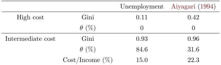
The top-panel of the table displays the resulting characteristics in case of high
partic-ipation costs. In this setting, there are no households that enter in the contingent asset
market and, therefore, the fraction of insured agents, or equivalently the fraction of total
insured income, is zero. The two calibrations imply rather low level of inequality, as
indi-cated by a wealth Gini index of 0.11 for the unemployment economy and of 0.42 for the
Aiyagari (1994) economy. The bottom-panel of the table reports the same equilibrium
statistics in the presence of intermediate levels of participation costs. When participation
costs are not excessively high, the degree of partial insurance as well as the wealth Gini
13The calibration for theAiyagari(1994) model is as in p.19 ofDavila et al.(2012). The coefficient of
Unemployment Aiyagari (1994) High cost Gini 0.11 0.42
θ (%) 0 0
Intermediate cost Gini 0.93 0.96
θ (%) 84.6 31.6
[image:26.595.115.480.73.181.2]Cost/Income (%) 15.0 22.3
Table 3 – Degree of partial insurance
coefficient increase. Yet, the relationship between the degree of partial insurance and
the increased level of inequality is not trivial and is calibration-dependent: even a small
share of partial insurance, which corresponds to a small share of participation, around 30
percent, as in the case of Aiyagari (1994) economy, is able to skew the wealth
distribu-tion to provide with a Gini index similar to one observed in the U.S. data. In this case,
even with a minority of insured households, the equilibrium level of interest rate and the
social mobility effect described in the previous section give rich agents large incentives
to accumulate wealth. Interestingly, the unemployment economy implies a similar level
of inequality with a much larger participation rate, around 80 percent. In this setting,
the properties of the income process are such that even a small fraction of self-insured
household has strong incentives to accumulate a large amount of wealth.
Our definition of partial insurance can be linked to the one introduced inGuvenen and
Smith(2014). However, whereas their form of partial insurance is on the intensive margin
- agents can insure a fraction of their income, in our setting partial insurance is on the
extensive margin - agents can be insured or not. In their empirical work, Guvenen and
Smith(2014) estimates the fraction of partial insurance around 45 percent. In this section
we showed how the existence of participation costs, which leads to partial insurance, can
generated realistic level of wealth inequality together with degree of partial insurance
both above and below their estimated partial insurance level.
5.3
Participation Costs and Welfare
This subsection analyses the welfare properties of an economy with participation costs.
It is well-known that economies with idiosyncratic shocks are not necessarily constrained
Pareto efficient (cf.Carvajal and Polemarchakis,2011;Davila et al.,2012, among others)
in the sense that a central planner can do better than the market allocation when accessing
the same tools. The central idea of that result stems from a pecuniary externality arising
through factor prices (e.g. wages and interest rates): by accumulating more assets, agents
we developed in this paper, the same intuition applies for the accumulation of risk-free
assets as well as of contingent assets, as we discuss in this section.
Let us first define constrained Pareto efficiency in our setting. The central planner
solves the following problem:
Problem 3.
V(x) = max
B0(y,B,a),δ(y,B,a),a0(y,B,a)
Z
u
B+a1y=yl+wy−q
f(K)B0
(y, B, a)· · · · · · −δ(y, B, a) (q(K)a0(y, B, a) +κ)
dx+βV(x
0
),
s.t. x0 =T(x, Q(., y)), K = Z
(a+B)dx.
As inDavila et al.(2012), we consider equal weights for all agents as we are interested
in insurance and not in redistribution. Finally, we assume that the central planner is also
constrained to rule out allocation where she would be able to perfectly insure agents by
transfers.
The solution of Problem 3 allows us to obtain the following results:
Proposition 10. The planner’s problem solution is such that:
(i) For κ≤κ, the economy is constrained Pareto optimal.
(ii) For κ≥κ, the economy is constrained Pareto suboptimal.
Furthermore, the central planner’s solution features perfect insurance for some κ > κ. Otherwise, constrained efficient insurance is ambiguous.
Proof. See Appendix C.7 for the proof.
When participation costs are sufficiently low (κ ≤ κ), agents are fully insured and markets are completed both in the central planner’s solution and in the competitive
market solution. In this case, the competitive market solution is constrained Pareto
optimal.
When participation costs increases to an intermediate level, there is no more full
insurance and the economy transits in the partial-insurance equilibrium. In this case,
a pecuniary externality arises through asset prices as already noted by Carvajal and
Polemarchakis (2011) or Davila et al. (2012). We show that this externality also arises
in the insurance behavior: for intermediate values of participation costs, agents insure
less in the competitive equilibrium compared with the central planner’s allocation. This
translates into a lower risk-free rate and a lower level of aggregate insurance.
Nevertheless, when participation costs are sufficiently high so that the central planner
as noted by Davila et al. (2012), higher levels of capital can lead to more insurance as
they allow to redistribute wealth to agents at the bottom of the wealth distribution,
for whom labor is the main source of income. Insurance markets reduce the agents’
willingness to save and, therefore, the aggregate level of capital: as a result, insurance
through markets and through higher wages are competing with each other. In the end,
the degree of insurance in the central planner’s solution may be higher or lower compared
to the competitive market allocation depending on the relative size of these two insurance
mechanisms.
We show in the appendix that the constrained efficient solution is characterized by
equations that differ from the competitive market allocation only by some additional
terms depending on factor prices, as inDavila et al.(2012) (See AppendixC.7). By
com-puting these additional terms, we are then able to determine whether there is too much
or too little participation compared with the efficient allocation. With the unemployment
economy calibration, this leads to the results presented in Table 4. In the intermediate
cost case, wealth inequalities are large and redistribution is more effective through higher
wages and more capital and so, through less insurance. This is not the case in the high
cost case, where agents gain from a higher interest rate and, then, a lower stock of capital.
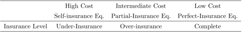
[image:28.595.91.507.402.458.2]High Cost Intermediate Cost Low Cost Self-insurance Eq. Partial-Insurance Eq. Perfect-Insurance Eq. Insurance Level Under-Insurance Over-insurance Complete
Table 4 – Constrained efficiency of insurance
6
Evidence on partial insurance and consumption
smoothing
In this section, we investigate the extensive margin of partial insurance and
con-sumption smoothing. In particular, we test an implication of our model, which is the
non-monotonic distribution of insurance. Recall, that Corollary 5 states that with
in-termediate participation costs the economy features a partial-insurance equilibrium in
which poor households are non-insured, middle-class households are perfectly insured,
and richer household are only partially insured. In this section, we confirm that result by
directly analyzing consumption data, income, and wealth Italian data.
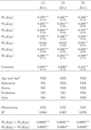
∆ logcit=α1+
N X
j=1
αj(Dj∆ logyit) +βXit+it, (3)
where Dj, with j = 1, .., N, is a dummy indicating groups of increasing wealth. The estimates αj, with j = 1, .., N, are the coefficients of interest, since they measure the degree of consumption insurance for a given wealth category. We estimate the regression
in (3) by using the Bank of Italy Survey of Households’ Income and Wealth (SHIW) panel
data in the period 2006-2008, since it uniquely provides information about the level of
wealth of the households. We consider seven wealth categories, identified by the following
six percentiles: 10, 25, 50, 75, 85, 95, to explore the insurance level of at the extremes of
the distribution. We consider three different specifications that control for age, education,
lifecycle (status), type of profession, and geographical areas. The results are presented
in Table 5. The estimation confirms the non-monotonic degree of consumption insurance
as predicted by our model. Poor households are largely uninsured; when the wealth
increases, consumption insurance improves. The 5th wealth level (75-85 percentile) is
perfectly insured, since the coefficient linking income growth to consumption growth is
not significantly different from zero. Importantly, at the top of the wealth distribution
the households are only partial insured. At the bottom of the table, we report the
p-values of the hypothesis that test these predictions. First, the insurance coefficient
for the poorest wealth category is significantly different than the next higher wealth
category at 1 percent significance level. Indeed, that means that the poorest category are
significantly less insured. Second, the insurance coefficient for the 5th wealth category is
significantly different than the one for the highest wealth category at 1 percent significance
level. This means that, there is a statistically significant difference between the low
income relationship for the middle class and the larger
consumption-to-income relationship for the richest households.
Additional evidence on non-monotone insurance. Even though it has not been
documented on its own, our non-monotonicity result is consistent with recent findings
based on improvements of the treatment of U.S. CEX data as inAguiar and Bils(2015),
who show that taking into account rich households’ specific consumption increases the
volatility of their consumption and hence aggregate consumption inequality. Our result is
also consistent with the non-monotone marginal propensity of consumption across wealth
during the Great Recession as estimated by Krueger et al. (2015).
It is also possible to confirm the non-monotonic insurance behavior by checking
whether agents actually purchase insurance. For example, Parsons et al. (2015)