warwick.ac.uk/lib-publications
A Thesis Submitted for the Degree of PhD at the University of Warwick
Permanent WRAP URL:
http://wrap.warwick.ac.uk/91939
Copyright and reuse:
This thesis is made available online and is protected by original copyright.
Please scroll down to view the document itself.
Please refer to the repository record for this item for information to help you to cite it.
Our policy information is available from the repository home page.
M A
E
G NS
I
T A T
MOLEM
U N
IVER
SITAS WARWICEN SIS
Predicting Context and Locations from
Geospatial Trajectories
by
Alasdair Thomason
A thesis submitted to The University of Warwick
in partial fulfilment of the requirements
for admission to the degree of
Doctor of Philosophy
Department of Computer Science
The University of Warwick
Abstract
Adapting environments to the needs and preferences of their inhabitants is
be-coming increasingly important as the world population continues to grow. One
way in which this can be achieved is through the provision of timely information,
as well as through the personalisation of services. Providing personalisation in
this way requires an understanding of both the historical and future actions
of individuals. Using geospatial trajectories collected from personal
location-aware hardware, e.g. smartphones, as a basis, this thesis explores the extent to
which we can leverage the latent knowledge in such trajectories to understand
the historic and future behaviours of individuals.
In this thesis, several machine learning tools for the task are presented,
including the development of a novel clustering algorithm that can identify
locations where people spend their time while disregarding noise. The knowledge
exposed by such a system is then enhanced with a procedure for identifying
geographic features that the person was interacting with, providing information
on what the user may have been doing at that time. Interactions with these
features are subsequently used as a basis for understanding user actions through
a new contextual clustering approach that identifies periods of time where the
user may have been performing similar activities or have had similar goals.
Combined, the presented techniques provide a basis for learning about the
actions of individuals. To further enhance this knowledge, however, the research
presented in this thesis concludes with the presentation of a new machine
learn-ing model capable of summarislearn-ing and predictlearn-ing the future context of
indi-viduals where only geospatial trajectories are required to be collected from the
user. Throughout this work, the potential benefits o↵ered by geospatial
trajec-tories are explored, with thorough explorations and evaluations of the proposed
Acknowledgements
The work contained in this thesis has been influenced by many people, both
academically through guidance and suggestions, but also through support,
en-couragement and friendship. Without these people, this thesis would not exist.
Firstly, my thanks go to my supervisors, Dr Nathan Griffiths and Dr Victor
Sanchez, who have provided unparalleled support and guidance throughout my
time as a postgraduate student. It is their feedback and ideas that have guided
the work over the past 3.5 years into a coherent thesis and helped me develop
many skills along the way, and I am indebted to them for this.
Secondly, I would like to thank my fellow postgraduate students, both past
and present, for their endless supply of lunchtime distractions, amusement and
discussion. In addition, many other members of the department have helped
me through the years, providing advice, resources and assistance: my advisors,
Dr Abhir Bhalerao and Dr Mike Joy, the technical team of Richard
Cunning-ham, Adam Hancox, Rod Moore, Roger Packwood and Paul Williamson, and
the administration team of Jane Clarke, Ruth Cooper, Sharon Howard, Lynn
McLean, Catherine Pillet and Gillian Reeves-Brown along with many others.
Finally, but by no means least importantly, I wish to thank my family and
friends outside the department: my parents for providing me with the
educa-tion and encouragement to go to university, as well as support throughout my
time here and invaluable proof-reading services; my siblings, Elly and Dave, for
providing much needed distraction from work; Christian, Danielle, and Louise,
amongst others, for support and friendship whenever it was needed.
Although I will not list their names to protect their anonymity, I am also
extremely grateful to the individuals who provided me with data for this work
by allowing me to track their movements through their smartphones. The data
Declarations
The research presented in this thesis is the work of the author and has not
been submitted for consideration at another institution. The work was funded
by an EPSRC Doctoral Training Partnership Studentship, and parts of this
thesis have been published in the following journals, collections and conference
proceedings:
• Thomason, Alasdair; Griffiths, Nathan; and Leeke, Matthew. 2015a.
Ex-tracting Meaningful User Locations from Temporally Annotated
Geospa-tial Data. In Internet of Things: IoT Infrastructures, volume 151 of
LNICST, pages 84–90. Springer. doi: 10.1007/978-3-319-19743-2 13
This paper presents the initial form of the Gradient-based Visit
Extrac-tor (GVE) algorithm, which forms the basis for Chapter 4.
• Thomason, Alasdair; Griffiths, Nathan; and Sanchez, Victor. 2015b.
Pa-rameter Optimisation for Location Extraction and Prediction
Applica-tions. In Proceedings of the 2015 IEEE International Conference on
Pervasive Intelligence and Computing, pages 2173–2180, Liverpool. doi:
10.1109/CIT/IUCC/DASC/PICOM.2015.322
An exploration of automatic parameter optimisation for extracting and
predicting locations over geospatial trajectories, included in Chapter 4,
Section 4.5
• Thomason, Alasdair; Leeke, Matthew; and Griffiths, Nathan. 2015c.
Understanding the Impact of Data Sparsity and Duration for
Loca-tion PredicLoca-tion ApplicaLoca-tions. In Internet of Things: IoT
Infrastruc-tures, volume 151 of LNICST, pages 192–197. Springer. doi: 10.1007/
This paper presents an investigation into understanding how properties of
geospatial data impact predictions made over the same data. Although
not part of the core focus of this thesis, the results are briefly mentioned
in Chapter 4, Section 4.5.2.
• Thomason, Alasdair; Griffiths, Nathan; and Sanchez, Victor. 2016a.
Iden-tifying Locations from Geospatial Trajectories. Journal of Computer and
System Sciences, 82(4):566–581. doi: 10.1016/j.jcss.2015.10.005
An extension of [Thomason et al., 2015a], that presents an expanded
Gradient-based Visit Extractor (GVE) algorithm and significantly more
in-depth evaluation, again forming the basis for Chapter 4.
• Thomason, Alasdair; Griffiths, Nathan; and Sanchez, Victor. 2016b.
Con-text Trees: Augmenting Geospatial Trajectories with ConCon-text. ACM
Transactions on Information Systems, 35(2):14:1–14:37. doi: 10.1145/
2978578
This work presents and evaluates the Context Tree data structure. Part
of the generation procedure forms the basis for Chapter 5, with the
re-mainder of the work being included in Chapter 6.
• Thomason, Alasdair; Griffiths, Nathan; and Sanchez, Victor. 2016c.
Pre-dicting Interactions and Contexts with Context Trees. InProceedings of
the 24th ACM SIGSPATIAL International Conference on Advances in
Geographic Information Systems, pages 46:1–46:4, San Francisco. doi:
10.1145/2996913.2996993
This paper presents the Predictive Context Tree (PCT) model, a
hierar-chical classifier that predicts future contexts of individuals. The work also
presents a foundation for predicting the geographic features a person will
interact with, providing the basis for Chapter 7, as well as reinforcing the
Additional parts of this thesis are contained in manuscripts currently under
review for publication:
• Thomason, Alasdair; Griffiths, Nathan; and Sanchez, Victor. 2016d.
The Predictive Context Tree: Predicting Contexts and Interactions.
arXiv:1610.01381 (pre-print)
This work is an extension to [Thomason et al., 2016c], and thus parts of
it are included in Chapters 5 and 7.
Implementations of all algorithms and tools referenced in this thesis have been
made available at: github.com/csukai/position.
Data
Portions of the research in this thesis used the Nokia Mobile Data Challenge
(MDC) Dataset made available by Idiap Research Institute, Switzerland and
owned by Nokia [Kiukkonen et al., 2010; Laurila et al., 2012], in addition to data
collected from members of the Department of Computer Science, University of
Abbreviations
ANN Artificial Neural Network
AUROC Area Under the Receiver Operating Characteristic Curve
DBN Dynamic Bayesian Network
DBSCAN Density-Based Spatial Clustering of Applications with Noise
GLONASS Global Navigation Satellite System
GPS Global Positioning System
GVE Gradient-based Visit Extractor
HCD Hybrid Contextual Distance Metric
HMM Hidden Markov Model
LUI Land Usage Identification Procedure
MAE Mean Absolute Error
MDC Nokia Mobile Data Challenge Dataset
OSM OpenStreetMap
PCA Principal Component Analysis
PCT Predictive Context Tree
STA Spatio-Temporal Activity
Notation
T Geospatial trajectory: T ={p(1), p(2), p(3), ..., p(n)
p Trajectory point: p(i) = (x(i), y(i), t(i), (i))
x(i) Thexcoordinate of pointi, typically degrees of longitude
y(i) They coordinate of pointi, typically degrees of latitude
t(i) The time component of pointi
(i) The accuracy value of pointi, typically maximum likely deviation
measured in metres
V Set of visits: V ={v(1), v(2), v(3), ..., v(n)}
v Individual visit: v(i) = (p(i), t(i), d(i)); a period of low mobility
extracted solely from geospatial trajectories
(i) The position of visiti
d(i) The duration of visiti
l Significant location: a cluster ofvisits based on geographical
proximity.
f Geographic feature: a physical entity in the world that has some
purpose, e.g. a building, road, public amenity
e Element: a representation of a geographical feature from a dataset
i Interaction: a period of time spent interacting with, or within, an
Contents
Abstract ii
Acknowledgements iii
Declarations iv
Abbreviations vii
Notation viii
List of Figures xviii
List of Tables xx
List of Algorithms xxi
1 Introduction 1
1.1 Understanding People from Data . . . 1
1.2 Geospatial Trajectories . . . 2
1.3 Problem Statement and Contributions . . . 3
1.4 Code and Algorithms . . . 5
1.5 Thesis Structure . . . 5
2 Background and Related Work 7 2.1 Managing and Collecting Data . . . 8
2.1.1 Resource Utilisation . . . 8
2.1.2 Privacy . . . 9
2.1.3 Synthetic Data . . . 10
2.1.4 Ground Truths . . . 10
2.2.1 Reducing Uncertainty . . . 11
2.2.2 Change-point Detection . . . 12
2.2.3 Visit Extraction . . . 12
2.3 Significant Locations . . . 14
2.3.1 Extracting Locations . . . 15
2.3.2 Labelling and Recommending Locations . . . 18
2.4 Location Prediction . . . 19
2.4.1 Cell-tower Handover . . . 20
2.4.2 Next Location Prediction . . . 22
2.4.3 Future Location Prediction . . . 24
2.4.4 Destination Prediction . . . 25
2.5 Contexts and Activities . . . 25
2.5.1 Identifying Activities . . . 25
2.5.2 Identifying Contexts . . . 27
2.5.3 Predicting Future Contexts . . . 27
2.6 Applications of Geospatial Systems . . . 28
2.6.1 Transport . . . 28
2.6.2 Trajectory Similarity Identification . . . 29
2.6.3 Anomaly Identification . . . 30
2.7 Summary . . . 30
3 Datasets 32 3.1 Geospatial Trajectories . . . 32
3.1.1 Individuals . . . 32
3.1.2 Other Entities . . . 35
3.1.3 The Warwick Dataset . . . 35
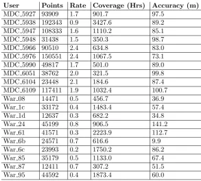
3.1.4 Trajectories Selected for Evaluation . . . 36
3.2 Land Usage Data . . . 38
4 Identifying Visits from Geospatial Trajectories 41
4.1 Introduction . . . 41
4.1.1 Visit and Location Identification . . . 42
4.1.2 Use Cases . . . 44
4.2 Related Work . . . 44
4.2.1 Visit Extraction . . . 45
4.2.2 Visit Clustering . . . 46
4.2.3 Location Prediction . . . 46
4.2.4 Parameter Optimisation . . . 47
4.3 The Gradient-based Visit Extractor (GVE) . . . 48
4.3.1 Clustering Visits into Locations . . . 51
4.3.2 Properties of Extracted Visits . . . 52
4.4 Evaluation: Comparison to Thresholding and the Spatio-Temporal Activity (STA) Extraction Algorithm . . . 64
4.4.1 Accurate Visits Use Case . . . 65
4.4.2 Location Properties Use Case . . . 70
4.5 Predicting Over Extracted Locations . . . 74
4.5.1 Evaluation Metric . . . 76
4.5.2 Optimisation Methodology . . . 79
4.5.3 Results and Analysis . . . 81
4.6 Conclusion . . . 86
5 Augmenting Geospatial Trajectories with Land Usage Data 87 5.1 Introduction . . . 87
5.2 Related Work . . . 89
5.3 Land Usage Identification (LUI) Procedure . . . 90
5.3.1 Augmentation . . . 91
5.3.2 Scoring and Filtering . . . 92
5.3.3 Summarisation . . . 94
5.4.1 Data . . . 96
5.4.2 Exploring the Augmentation Procedure . . . 96
5.4.3 Comparison with Extracted Locations . . . 101
5.4.4 Predicting Land Usage Interactions . . . 107
5.5 Summary and Conclusion . . . 111
6 The Context Tree 114 6.1 Introduction . . . 114
6.2 Related Work . . . 115
6.3 Identifying Contexts Through Clustering . . . 117
6.3.1 Augmentation, Filtering, and Summarisation . . . 120
6.3.2 Building Clusters . . . 121
6.3.3 Contextual Distance Metrics . . . 123
6.3.4 Hierarchical Clustering . . . 126
6.3.5 Context Tree Pruning . . . 127
6.4 Case Study . . . 131
6.4.1 Methodology . . . 131
6.4.2 Filtering and Summarising . . . 133
6.4.3 Clustering . . . 140
6.4.4 Pruning Evaluation . . . 148
6.5 Summary and Conclusion . . . 152
7 Applying Context Trees: The Predictive Context Tree 153 7.1 Introduction . . . 153
7.2 Related Work . . . 154
7.3 The Predictive Context Tree (PCT) . . . 155
7.3.1 Training a PCT . . . 157
7.4 Evaluation . . . 160
7.4.1 Constructing Predictive Context Trees . . . 161
7.4.2 Evaluating Predictions . . . 161
7.5 Summary and Conclusion . . . 178
8 Discussion and Conclusion 179 8.1 Contribution Summary and Future Work . . . 180
8.2 Final Remarks . . . 187
References 189 Appendices 212 A Visit Extraction . . . 213
B Land Usage Augmentation . . . 216
C The Predictive Context Tree (PCT) . . . 217
List of Figures
4.1 Visit extraction is performed over geospatial trajectories (left) to
identify periods of low mobility (right). . . 42
4.2 The relationship between parameters↵and and the number of
visits identified for the GVE algorithm. . . 54
4.3 The e↵ect on proportion of trajectory points designated asnoise
when varying↵and for the GVE algorithm. . . 56
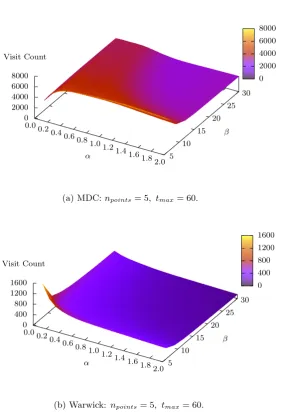
4.4 The e↵ect of the parametersnpoints andtmax on the GVE
algo-rithm. . . 58
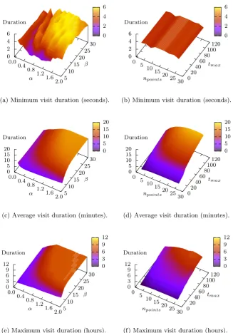
4.5 The e↵ect of parameters on the minimum, average, and maximum
length of extracted visits for the GVE algorithm. . . 59
4.6 The e↵ect of DBSCAN’sepsandminpts parameters on the
num-ber of locations clustered from visits identified using GVE. . . 61
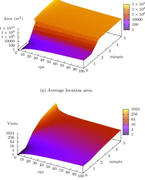
4.7 The e↵ect of DBSCAN’sepsandminpts parameters on the
aver-age size of locations and the averaver-age number of visits per location
for the MDC dataset on visits identified using GVE. . . 62
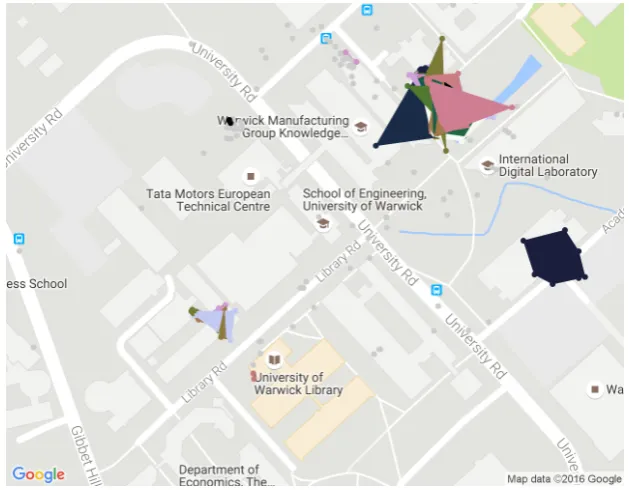
4.8 Example visits extracted for Warwick user08. . . 69
4.9 Ground truth locations identified for Warwick user61. . . 74
4.10 Extracted clusters that maximise Dice’s coefficient relative to the
ground truth for Warwick user61. . . 75
4.11 Example simulated annealing runs showing error against time. . 82
4.12 Relationship between the proposed error metric and properties
of extracted locations and predictions. . . 83
4.13 Number of runs conducted that produce locations with di↵erent
average sizes. . . 83
4.14 The e↵ect of the optimisation procedure’s parameters on
5.1 Example of the trajectory augmentation procedure. . . 91
5.2 Examples of the data at each stage of the augmentation, filtering,
and summarisation processes. . . 97
5.3 The distribution of normalised element scores before element
se-lection takes place as part of the filtering procedure. . . 98
5.4 The e↵ect of accuracy on number of elements, pre- and
post-filtering, for di↵erent users’ data. . . 99
5.5 The e↵ect of on the number of unique elements identified through
the LUI procedure. . . 100
5.6 The e↵ect oftmaxon the summarisation procedure. . . 102
5.7 The e↵ect ofdmin on the summarisation procedure. . . 102
5.8 Average numbers of interactions and locations extracted for the
LUI procedure and location extraction techniques. . . 104
5.9 Average duration of interactions for the LUI procedure and
loca-tion extracloca-tion techniques. . . 104
5.10 Average size of elements and locations for the LUI procedure and
location extraction techniques. . . 105
5.11 Average size of elements and locations for the LUI procedure
and location extraction techniques, where land usage elements
are restricted by both radius and area. . . 107
5.12 The e↵ect ofdmin on predictive accuracy. . . 109
5.13 The e↵ect of dmin on predictive accuracy for the restricted land
usage elements. . . 112
5.14 Predictive accuracies for locations extracted with thresholding,
and land usage elements identified through the LUI procedure,
when predicting with SVMs over the MDC dataset. . . 112
6.1 An abstract representation of a Context Tree, in which the
simi-larity of nodes increases with depth. . . 117
6.3 An example of how clusters are merged together when generating
Context Trees. . . 123
6.4 An example of a pruned Context Tree. . . 128
6.5 An extract of a Context Tree generated using real data. . . 132
6.6 The e↵ect of element filtering on tag key similarity from a single user’s data, both pre- and post-filtering. . . 134
6.7 The e↵ect of n on number of land usage interactions identified when constructing Context Trees. . . 134
6.8 Partial ground-truth data I. . . 136
6.9 Partial ground-truth data II. . . 136
6.10 Partial ground-truth data III. . . 137
6.11 The proportion of tags identified as relevant through the ground truth comparison. . . 140
6.12 The e↵ect of on the number of tree nodes in a Context Tree. . 141
6.13 Example Context Tree: Geographic clustering. . . 142
6.14 Example Context Tree: Temporal clustering. . . 142
6.15 Example Context Tree: Semantic clustering. . . 143
6.16 Example Context Tree: Feature-based clustering. . . 143
6.17 Example Context Tree: Hybrid clustering. . . 144
6.18 Example data from a single user showing the proportion of new land usage elements encountered each day. . . 146
6.19 The relationship between amount of training data and number of tree nodes in a Context Tree. . . 147
6.20 The e↵ect of✓ on number of nodes in a sample Context Tree. . . 149
6.21 The e↵ect of⇠on number of nodes in a sample Context Tree. . . 150
6.22 Example Context Trees pruned with di↵erent values of✓. . . 151
7.1 Abstract representation of a PCT. . . 156
7.2 Classification methods for PCTs. . . 158
7.4 Example classification labels for di↵erent predicted sets through
the PCT . . . 163
7.5 The e↵ect ofdmin on predictive accuracy. . . 165
7.6 Predictive accuracy of the PCT, considering element prediction. . 165
7.7 Predictive accuracy of the PCT, considering context prediction. . 166
7.8 Comparison of di↵erent predictive techniques, considering
ex-tracted locations, land usage elements, and contexts. . . 167
7.9 The e↵ect of parameters Ts and on context prediction. . . 168
7.10 Predictive accuracies for the di↵erent prediction techniques for
the MDC dataset. . . 170
7.11 Comparisons of predictive accuracies for the MDC data with and
without truncated periods for land usage and element PCT
pre-diction. . . 171
7.12 Predictive accuracies observed when using pruned Context Trees. 173
7.13 Predictive accuracies obtained when using di↵erent probabilistic
models as classifiers in the PCT. . . 174
7.14 The e↵ect ofnon predictive accuracy for the multi-element
Con-text Tree. . . 176
A.1 The e↵ect of the parametersnpoints andtmax on the GVE
algo-rithm over the Warwick dataset. . . 213
A.2 The e↵ect of parameters on the minimum, average, and maximum
length of extracted visits for the GVE algorithm and the Warwick
dataset. . . 214
A.3 The e↵ect of DBSCAN’sepsandminpts parameters on the
aver-age size of locations and the averaver-age number of visits per location
for the Warwick dataset on visits identified using GVE. . . 215
A.4 Summaries of comparisons between land usage elements
identi-fied through the LUI procedure and locations extracted through
A.5 The e↵ect of parametersTsand on context prediction over the
MDC dataset. . . 217
A.6 Predictive accuracies observed when using pruned Context Trees
generated from MDC data. . . 218
A.7 Predictive accuracies obtained when using di↵erent probabilistic
models as classifiers in the PCT over the MDC data. . . 219
A.8 The e↵ect ofnon predictive accuracy for the multi-element
Con-text Tree over MDC data. . . 220
A.9 Summaries of comparisons between land usage elements
identi-fied through the LUI procedure and locations extracted through
location extraction techniques over the MDC dataset with
trun-cated periods. . . 221
A.10 Predictive accuracies for locations extracted with thresholding,
and land usage elements identified through the LUI procedure,
when predicting with SVMs over the MDC dataset with
trun-cated periods. . . 222
A.11 Predictive accuracies for the di↵erent prediction techniques for
List of Tables
3.1 Summary of users selected from the Warwick and MDC datasets. 38
4.1 Parameters considered for the GVE algorithm as part of the
pa-rameter exploration. . . 52
4.2 Parameters considered for DBSCAN as part of the parameter exploration. . . 63
4.3 Summarised e↵ects of the GVE algorithm’s parameters as each parameter is increased. . . 64
4.4 Summarised e↵ects of the Density-Based Spatial Clustering of Applications with Noise (DBSCAN) algorithm’s parameters as each parameter is increased. . . 64
4.5 Parameter values used for evaluating visit extraction procedures. 67 4.6 Summary of parameter sets that match expected values for dif-ferent visit extraction techniques. . . 68
4.7 Summaries of properties of the visits shown in Figure 4.8. . . 70
4.8 Parameter increments selected for the optimisation procedure. . . 71
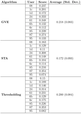
4.9 Summary of how well each visit extraction technique performs relative to a partial ground truth. . . 73
5.1 Example augmented trajectory. . . 92
5.2 Example summarised trajectory. . . 92
5.3 Summary of point accuracy for each user of both datasets. . . 100
5.4 Total visit and interaction time in days for the di↵erent tech-niques, averaged over the Warwick users. . . 106
5.5 Average area of extracted locations and identified land usage el-ements (both unrestricted and restricted areas). . . 108
5.7 Accuracy of di↵erent techniques for HMMs. . . 110
5.8 Accuracy of di↵erent techniques for SVMs over the MDC dataset. 113
6.1 Summary of tags and frequency count for each type of ground
truth interaction. . . 139
7.1 Accuracy of the PCT when predicting contexts for the Warwick
dataset. . . 166
7.2 Comparison of di↵erent predictive techniques. . . 167
7.3 Comparison of di↵erent predictive techniques over MDC data. . . 170
7.4 Accuracies achieved using di↵erent classification models in the
PCT when predicting elements. . . 175
7.5 Accuracies achieved using di↵erent classification models in the
PCT when predicting contexts. . . 175
7.6 Accuracy of the PCT when predicting multiple elements over the
Warwick dataset. . . 177
7.7 Accuracy of the PCT when predicting multiple contexts over the
List of Algorithms
1 Gradient-based Visit Extractor (GVE) algorithm. . . 49
2 The Land Usage Identification (LUI) procedure’s bu↵er
manage-ment process. . . 93
3 The Land Usage Identification (LUI) procedure’s summarisation
algorithm. . . 94
4 Modified summarisation procedure for overlapping interactions. . 121
5 The Predictive Context Tree (PCT)’s agglomerative hierarchical
CHAPTER
1
Introduction
Adapting environments to the needs and preferences of their inhabitants is
be-coming increasingly important as the world population continues to grow. With
the majority of people now living in urban environments1, the provision of smart
services and utilities has an unprecedented ability to improve the lives of
indi-viduals and societies. This can be realised through the provision of timely and
useful information, control of automated systems, and even utilities and transit
management at city-scale. In order to provide personalised services, we first
require the ability to model and understand the behaviours, interactions and
patterns of city inhabitants. One way in which this can be achieved is to collect
vast amounts of data from individuals, or the devices they carry. However, the
collection of such data would typically be invasive and require additional sensor
devices to be carried. Instead, we focus our work on geospatial trajectories that
can be collected from smartphones, routinely carried by the majority of the
population2.
1.1
Understanding People from Data
Understanding and modelling the behaviour of individuals can be performed in
various ways, from monitoring how people interact with their devices [LiKamWa
et al., 2011, 2013; Shye et al., 2010; Wang et al., 2014] and the internet [Alhindi
et al., 2015; Ashman et al., 2009; Gossen et al., 2013; Popescu, 2010; Steichen
et al., 2012; Zhang, 2013], through to analysing footage from video cameras
[Brax, 2008; Janoos et al., 2007; Kim et al., 2010; Sillito and Fisher, 2008], or
1data.worldbank.org/indicator/SP.URB.TOTL.IN.ZS
1. Introduction
data from heart-rate monitors and other low-level sensors [Choudhury et al.,
2008; Lee and Mase, 2002; Lester et al., 2005; Morris and Trivedi, 2011;
Pirt-tikangas et al., 2006; Ravi et al., 2005]. In addition to these sources, online
pro-filing has increasingly been used to understand the preferences of individuals,
however, many activities are conducted o↵-line and therefore require additional
data in order to characterise. Such data could come from video and other
low-level sensors, which may be able to identify physical activities the user conducts,
but such data is not always available, and so would cover only limited parts of
a person’s day.
Aiming for more continuous data collection, in a manner that does not
sig-nificantly inconvenience the user, we instead focus our attention on geospatial
trajectories. These trajectories are sequences of data points that link an
en-tity (e.g. a person, device, vehicle, etc.) to a specific geographic location at a
specific time, and can be collected from any manner of sources. Many devices
are now location-aware, being capable of sensing their current location. Such
devices include smartphones, in-car navigation devices, and even watches. The
continuous collection and use of geospatial trajectories is becoming increasingly
possible, with the goal of better personalising the services these devices o↵er to
their users. Furthermore, trajectories can also be collected without any action
required of the user though cell tower connections (i.e. by monitoring the towers
in range of a cellular device), or through credit card usage, amongst many other
methods. These are all minimally invasive to the user, but provide information
on which to better learn and understand the person to whom the device belongs.
1.2
Geospatial Trajectories
Regardless of their source or how they are collected, geospatial trajectories are
sequences of data points associated with a person or other entity. Each data
1. Introduction
value that represents the uncertainty in the location measurement:
T ={p(1), p(2), p(3), ..., p(n)} p(i) = (x(i), y(i), t(i), (i)) (1.1)
Where T is a geospatial trajectory consisting of n points. p(i) is theith
tra-jectory point comprising of location,x(i) andy(i), timet(i) and accuracy (i),
representing the maximum likely deviation from the recorded location, usually
measured in metres. While it is not strictly necessary for the location to be
recorded as latitude and longitude, this is the most convenient way to
repre-sent a physical location, and so we assume that all geospatial trajectories are
recorded in this manner. A vast amount of latent knowledge is present in such
trajectories; it is the task of the remainder of this thesis to discuss existing
approaches of leveraging such knowledge, as well as presenting new methods.
1.3
Problem Statement and Contributions
This thesis aims to explore the potential o↵ered by geospatial trajectories to
the task of understanding individuals through machine learning. Specifically,
the problem statement is: Can a technique be developed to predict the
future actions, in terms of location and context, of individuals that
makes use of data available after collection, but requires only
geospa-tial trajectories to be collected from the individuals themselves? While
exploring this problem, the following contributions are made by this thesis:
1. Improving on current algorithms for identifying periods of low
mobility (i.e. when little motion is present) in geospatial
trajec-tories for the purpose of identifying locations meaningful to the
individual.
TheGradient-based Visit Extractor (GVE)is an algorithm for
iden-tifying periods of low mobility from geospatial trajectories, for the purpose
1. Introduction
algorithm is an improvement on existing techniques as it is more resilient
to noise and places fewer limitations on the extracted time periods. This
algorithm is combined with an analysis of the properties of the extracted
visits and the impact these properties have on a sample application, that
of location prediction. Such an evaluation is lacking in previous work.
Fur-thermore, additional techniques to aid in visit extraction and prediction
are proposed, including a method for automatic parameter optimisation
for extraction and prediction.
2. Developing a technique for the identification of geographic
fea-tures with which an entity interacts (e.g. specific buildings).
While extracting locations from geospatial trajectories produce arbitrary
shaped clusters, we propose theLand Usage Identification (LUI)
pro-cedure, as a method for augmenting trajectories with information on
geo-graphic features extracted from a dataset, referred to asland-usage data.
These augmented trajectories are then subjected to a filtering procedure
to identify geographic features with which an individual, or other entity,
interacted, providing a basis for understanding the type of places at which
a person spends their time.
3. Establishing a data structure for identifying and summarising
contexts from augmented geospatial trajectories to identify
pe-riods of time with similar goals, desires and intentions.
TheContext Treeis a hierarchical data structure with a generation
pro-cedure that identifies contexts based on the semantics of elements
encoun-tered and properties of the interaction with these elements. The Context
Tree itself provides a summary of the contexts an individual has been
immersed within.
4. Evaluating the data structure as a predictive model for
forecast-ing the future contexts and location interactions of individuals.
1. Introduction
a hierarchical classifier which is capable of predicting the future location
of interactions of individuals, achieving competitive accuracies when
com-pared with existing techniques. In addition to this, the PCT is able to
predict thecontext in which a person will be immersed to a high degree
of accuracy, o↵ering a platform on which to understand the future actions
of people, and thus provide useful and personalised services.
1.4
Code and Algorithms
Throughout this thesis, several tools, techniques and algorithms are developed
and applied to real-world geospatial trajectories. In order to encourage the use
of these techniques, the code used to generate results for this thesis, including
concrete implementations for each contribution, has been released under the
GNU GPL License3 and is located at: github.com/csukai/position.
1.5
Thesis Structure
The remainder of this thesis is structured as follows:
Chapter 2presents background knowledge relevant to the task of
under-standing people from geospatial trajectories. General machine learning topics
are discussed, and existing applications of geospatial systems are summarised.
Chapter 3discusses available datasets for this work, including specifics of
the datasets selected for use in this thesis. Additionally, this chapter sets out
data collection methodologies for the Warwick Dataset, which was collected to
overcome drawbacks of existing data available for research purposes.
Chapter 4 explores the potential for improving upon existing visit and
location extraction techniques, where the aim is to identify periods of low
mo-bility in geospatial trajectories and cluster these interactions into locations. The
chapter primarily presents theGradient-based Visit Extractor (GVE)algorithm
1. Introduction
that expands on previous algorithms for this task. The algorithm is then
evalu-ated thoroughly with respect to the properties of the identified interactions and
under the sample application of predicting future interactions. This chapter
also includes an exploration of the task of optimising parameters for extracting
locations using GVE, and provides a discussion on how this can be achieved.
Chapter 5investigates and proposes a method for identifying geographic
features being interacted with from geospatial trajectories augmented with land
usage data. This approach produces interactions that are similar in structure to
those identified by GVE, but map to single geographic features, thus providing
additional information in the form of knowledge about the type and properties of
the feature being interacted with. The interactions are evaluated using existing
machine learning techniques that have been demonstrated to be applicable to
location prediction, with a comparison presented between extracted locations
and identified elements.
Chapter 6 uses identified land usage elements as a basis for identifying
contexts through hierarchical clustering. The proposed Context Tree is a
hi-erarchical data structure and generation procedure that uses semantics and
properties of interactions with land usage elements to summarise user contexts.
This chapter presents the data structure, metrics, and algorithms for
construct-ing Context Trees, along with a technique for reducconstruct-ing the size of a Context
Tree through pruning.
Chapter 7builds upon the foundation o↵ered by Chapter 6, by presenting
a model for predicting the future interactions and contexts of an individual,
namely thePredictive Context Tree (PCT). This model is then evaluated with
respect to both predictions from extracted locations and predictions from
iden-tified land usage elements (Chapter 5).
Chapter 8concludes the thesis with a summary of the contributions made,
CHAPTER
2
Background and Related Work
Geospatial trajectories form the backbone of many location-aware systems and
services, and an increasing amount of research has focused on developing
tech-niques to leverage the knowledge latent in such trajectories. When coupled with
the now pervasive nature of location-sensing hardware, such as smartphones,
trajectories are an ideal basis for understanding, modelling, and predicting
hu-man behaviour.
In existing work, trajectories have been collected from dedicated devices
[Ashbrook and Starner, 2003], smartphones [Laurila et al., 2012], WiFi devices
[Burbey and Martin, 2008], social networks [Comito et al., 2016], vehicles [Hu
et al., 2015], smart buildings [Petzold et al., 2006; Roy et al., 2003], and mobile
phone cell networks [Bayir et al., 2009; Farrahi and Gatica-Perez, 2008b, 2009].
Using these trajectories as a basis for knowledge acquisition, research has
con-sidered many possible applications, including identifying locations meaningful
to individuals [Bamis and Savvides, 2011; Montoliu and Gatica-Perez, 2010],
predicting the future location of people [Ashbrook and Starner, 2003; Assam
and Seidl, 2013], determining transport methods [Patterson et al., 2003; Zheng
et al., 2008a], forecasting the destinations of journeys [Karimi and Liu, 2003;
Liao et al., 2007b], and even identifying similarities [Assam and Seidl, 2014;
Xiong and Lin, 2012] and anomalies between users [Chen et al., 2011a; Zhang
et al., 2011].
The remainder of this chapter explores these topics in depth, along with
2. Background and Related Work
2.1
Managing and Collecting Data
With various methods of collecting trajectories, ranging from manually writing
locations into a travel diary through to automatic logging from a portable device,
the properties of data available will vary. For this work, we focus primarily on
trajectories collected about individuals, typically from portable devices, but
they could also come from vehicular data recorders or from services such as
credit card or cellular telephone usage. This section discusses some challenges
relating to geospatial data and its collection.
2.1.1
Resource Utilisation
Determining the current location in a portable device can be achieved through
many technologies, such as the Global Positioning System (GPS), Global
Nav-igation Satellite System (GLONASS), WiFi positioning, and cell-tower
trian-gulation. The most accurate of these, GPS and GLONASS, have an accuracy
of approximately 5-10m in perfect conditions [GMV, 2011; Grimes, 2008], but
also requires the most power to determine position, and so existing work has
considered balancing the accuracy of collected data with the available resources
on the collection device.
In order to balance the requirement for accurate measurement with that of
preserving power, research has focused on optimising the data collection process.
Kiukkonen et al. [2010] present a state-based machine that transitions between
di↵erent collection rates and location determination methods based on sensor
readings, using WiFi base stations to indicate locations when available, and
adjusting the collection rate based on accelerometer readings (i.e. if the user is
moving, the collection rate is increased) at other times. Similarly, Chon et al.
[2011] present SmartDC, an application that aims to estimate when a user will
leave a current area and increase collection around this time, using a Markov
predictor, although this system is heavily reliant on the availability of WiFi
2. Background and Related Work
2.1.2
Privacy
Another concern when collecting geospatial data is privacy, the preservation of
which has long been the subject of research [Ackerman et al., 2001; Beresford
and Stajano, 2003; Kaasinen, 2003; Ljungstrand, 2001]. Methods for
preserv-ing privacy in location-aware systems include those focuspreserv-ing on the selective
obfuscation of originating users. An example of this is the application of ‘mix
zones’ where users can only be identified within certain regions, with user data
mixed together at other times [Beresford and Stajano, 2004], or providing the
users with fine control over what data can be shared and using intelligent
al-gorithms to determine how privacy would be reduced by sharing the user’s
location at any time [Boutsis and Kalogeraki, 2016]. Other solutions to the
pri-vacy preservation issue focus on enabling pripri-vacy-compromising computation
to be performed on client devices, eliminating the risk of intercept and
loca-tion inference [Marmasse and Schmandt, 2000], or the reducloca-tion of accuracy of
data, for example, the truncation of latitude and longitude values in the Nokia
Mobile Data Challenge (MDC) dataset [Laurila et al., 2012], discussed later in
Chapter 3. However, since some services necessitate the transmission of
loca-tion data, are too computaloca-tionally intensive for client devices, or require the
unambiguous identification of a user, the problem of preserving location privacy
in location-aware systems persists [Kaasinen, 2003].
Focusing on the reverse of these techniques, that of demonstrating the
pri-vacy implications of geospatial data, Rossi et al. [2015a; 2015b] explore
tech-niques for identifying users based on social media check-ins and GPS data. The
authors discover that check-ins to certain types of location reduce privacy more
than others, and that users have high uniqueness, thereby requiring very little
2. Background and Related Work
2.1.3
Synthetic Data
With the challenges associated with collecting real-world trajectory data, some
work chooses to generate synthetic data for evaluation instead [Giannotti et al.,
2007; Karimi and Liu, 2003; Lei et al., 2011; Wolfson and Yin, 2003; Zheng et al.,
2010c]. Creating synthetic data does, however, have its own problems. Firstly,
the ability for synthetic data to represent the distribution and patterns of real
data are limited, without a real-world dataset on which to base a probabilistic
model. Additionally, even with such data, creating a model that accurately
represents the movement patterns and characteristics of individuals is a
signifi-cant challenge. Several papers use synthetic data to evaluate location prediction
techniques [Bilurkar et al., 2002; Thanh and Phuong, 2007] and visit extraction
techniques [Bamis and Savvides, 2010], but fail to demonstrate the applicability
of the data they generate.
2.1.4
Ground Truths
For many techniques relating to extracting knowledge from data, collecting a
concrete ground truth is infeasible or dependant upon specific applications.
Sig-nificant location extraction, for example, can extract locations of di↵erent sizes
and scales and so no single ground truth can exist. Existing literature addresses
this by comparing the outputs from such techniques against certain metrics and
expectations. For instance, Guidotti et al. [2015] create synthetic trajectories
with known properties and devise metrics to compare extracted locations with
these properties. Much existing work additionally uses partial ground truths
constructed a posteriori from manually analysing the data and cross-referencing
with other data sources, such as maps and land usage information [Assam and
Seidl, 2014; Comito et al., 2016; Hoh et al., 2010; Lee et al., 2015; Sila-Nowicka
et al., 2015; Yan et al., 2013], or analysing video data about the study
par-ticipants to manually determine activities conducted [Lester et al., 2005]. In
2. Background and Related Work
by considering expected properties of the procedure with relation to input
pa-rameters [Bao et al., 2011].
2.2
Trajectory Processing
Once geospatial trajectories have been collected, they can be processed and
analysed to better understand people and their actions. This section presents
several existing methods for processing raw geospatial trajectories to provide a
foundation for understanding behaviour.
2.2.1
Reducing Uncertainty
Due to the di↵erent methods of collection of trajectories, each data point
typ-ically carries some amount of uncertainty. Reducing this uncertainty can be
achieved through filtering, outlier detection or tailored approaches such as
map-matching that uses known information about the environment to estimate the
true location of the entity [Qiu et al., 2013; Zheng, 2015]. Typical filtering
approaches include the Kalman filter [Cooper and Durrant-Whyte, 1994;
Mo-hamed and Schwarz, 1999; Zheng and Zhou, 2011], impulse response filter [Ge
et al., 2000], particle filter [Giremus et al., 2004; Wang et al., 2007], and moving
average filters [Tsai et al., 2004] to smooth out noisy data.
While most useful for vehicular trajectories, map-matching techniques aim
to reduce uncertainty by utilising additional information about the world to
determine the likely real location the trajectory point was recorded from. This
can be achieved by simply mapping the recorded point to the closest road [White
et al., 2000], or using more advanced filtering and estimation techniques (e.g.
the Kalman filter mentioned earlier) [Goh et al., 2012; Ochieng et al., 2003; Pink
2. Background and Related Work
2.2.2
Change-point Detection
Change-point detection can be applied to trajectories to identify the point at
which significant change occurs with the goal of partitioning the trajectory into
subtrajectories. Depending on the goal of the process, the criteria for selecting
change-points will vary, but typically includes monitoring for rapid changes in
speed, acceleration, or direction. Subtrajectories segmented in this manner have
been used for travel method identification, where the goal is to determine what
transportation mode (e.g. walking, cycling, driving) was in use for di↵erent
components of a journey [Liao et al., 2007b; Patterson et al., 2003; Zheng et al.,
2008a,b].
2.2.3
Visit Extraction
Visits, also referred to as stops or stays, are periods of a trajectory where the
entity is likely to have remained in a single location, for example a shop or house
for trajectories associated with individuals [Ashbrook and Starner, 2003], or a
parking garage or traffic queue for trajectories associated with vehicles [Yang
et al., 2013]. The identification of these visits enables applications to reason
about behaviour as a sequence of interactions with the environment [Andrienko
et al., 2011; Ashbrook and Starner, 2002, 2003; Bamis and Savvides, 2011;
Mon-toliu and Gatica-Perez, 2010]. After such interactions have been identified, we
are left with a sequence of visits performed by the entity:
V ={v(1), v(2), v(3), ..., v(n)} v(i) = ( (i), t(i), d(i)) (2.1)
Where V is a set of visits, with v(i) being an an individual visit associated
with a position, time and duration ( (i), t(i), d(i) respectively). For some
applications, the visits themselves can be ignored and only the periods of time
between them are considered. This may be useful in applications such as exercise
trackers where stationary periods are not of interest.
investiga-2. Background and Related Work
tion conducted by Ashbrook and Starner [2002; 2003] into identifying locations
meaningful to a user. From the collected data, Ashbrook and Starner observed
that the data loggers used did not function well indoors, as a GPS signal was
rarely available, and therefore treated periods of missing data as visits. This
approach is limited in that it assumes that all missing data is caused by a visit,
and visits cannot occur when data was collected. Indeed, the authors note that
the data logging devices were prone to run out of battery power, also
caus-ing a lack of data. Buildcaus-ing on this work, but assumcaus-ing a constant flow of
data, even when indoors, algorithms have been proposed that aim to identify
periods of low mobility from within trajectories. Relying on time and distance
thresholds, such algorithms typically operate by identifying subtrajectories that
contain points such that the subtrajectory, or visit, is smaller than a specified
radius (or, sometimes, that no consecutive points can be greater than a specified
distance apart) and the duration of the subtrajectory exceeds some threshold
[Andrienko et al., 2011, 2013; Hariharan and Toyama, 2004; Kang et al., 2004; Li
et al., 2008; Zheng et al., 2010b, 2009; Zhou et al., 2014]. Montoliu and
Gatica-Perez [2010] extend this technique, by adding an additional constraint that the
time between consecutive data points in the same visit must be bounded, with
the aim of preventing periods of missing data from being contained within a
visit. If data became unavailable at one time, and became available at a nearby
coordinate some time later, it is not possible to state with certainty that the
user remained stationary for the missing period. Another approach considered
for visit extraction makes use of the speed or velocity of the user, where low
speeds are considered indicative of a visit occurring [Lee et al., 2015; Palma
et al., 2008].
Although these techniques may overcome the issues caused by assuming
that a loss of GPS signal is equivalent to a visit, they all su↵er from a lack of
resilience to noise. In the thresholding approach, a single noise point outside
the visit radius will end a visit prematurely, and when considering velocity, it
2. Background and Related Work
user, thus also causing visits to be ended.
Aiming to overcome the drawbacks of existing approaches, by assuming noise
in the dataset, Bamis and Savvides [2010] present the Spatio-Temporal Activity
(STA) extraction algorithm. While the authors were specifically motivated by
identifying activities that repeat in cycles through extraction and clustering, the
first step of the algorithm, STA extraction, uses a definition of an activity that
is identical to our definition of a visit, and thus performs visit extraction. The
algorithm is similar to existing approaches in that it iterates over the trajectory
points, but uses a weighted averaging filter over the spatial component to reduce
the impact of noise before considering an activity to have ended. This technique,
however, does have several drawbacks and assumptions relating to the data,
for example, requiring evenly time-sliced data and a full data bu↵er before
consideration of a visit can occur, consequently imposing a minimum bound on
visit duration.
The topic of visit extraction is considered again later in Chapter 4, where an
algorithm is proposed that aims to overcome the drawbacks of the approaches
identified here. It is also considered in Chapter 5, where a novel approach to
identifying land usage elements interacted with by users is presented, designed
to replace traditional visit extraction for some domains.
2.3
Significant Locations
Significant, ormeaningful, locations form the backbone of many geospatial
ser-vices as they identify locations that have some meaning to the user. These
applications include predicting future visits to locations [Ashbrook and Starner,
2002, 2003; Fukano et al., 2013; Wang and Prabhala, 2012], predicting how long
a user will stay at a given location [Liu et al., 2013], as well as labelling
loca-tions with their likely meaning [Krumm and Rouhana, 2013]. Literature has
also considered the problem of predicting locations in which people will meet
2. Background and Related Work
new to a city based on the locations visited by others [Bao et al., 2015; Zheng
and Xie, 2010].
2.3.1
Extracting Locations
Section 2.2.3 discusses methods of identifying visits from geospatial
trajecto-ries, resulting in a sequence of such visits that each represents a period of time
in which a user remained in one place. The majority of existing work in
ex-tracting significant locations makes use of these identified visits by clustering
them together to determine visits that belong to the same location. This results
in a sequence of visits to locations, where unlike sets of trajectories or visits,
repeated visits to the same location, l(i), are possible, for example:
l(1)!l(2)!l(1)!l(3)!l(4)!l(2)!... (2.2)
Grouping visits into locations has been performed using unsupervised
learn-ing techniques such as clusterlearn-ing. Such algorithms are categorised into two
main types: Hierarchical and partitional. The aim of a hierarchical algorithm
is to create a tree-like structure of clusters with a single root cluster and di↵
er-ent scales of sub-cluster below. Partitional algorithms, in contrast, cluster the
entire dataset into discrete partitions at a single scale.
These types are further broken down into two categories of algorithms:
ag-glomerative anddivisive. Agglomerative algorithms start with each point as a
singleton cluster and continually perform rounds of merging until a termination
condition is met (bottom-up clustering). Divisive clustering, on the other hand,
starts with a single cluster containing all points and repeatedly splits the
clus-ters until some termination criterion is met (top-down clustering) [Jain et al.,
1999].
K-means are a family of iterative relocation algorithms that perform
ex-pectation maximisation to split the dataset into k clusters [MacQueen, 1967].
2. Background and Related Work
and continually make changes until the associated error ceases to change
sig-nificantly [Jain et al., 1999]. There are many di↵erent algorithms that use the
K-means approach, with MacQueen’s [1967] algorithm being the most widely
used. K-means is di↵erentiated from K-medoid algorithms in that the clusters
are described by their centre, while in K-medoid the clusters are described by an
existing point in the dataset that is as close as possible to the centre [Kaufman
and Rousseeuw, 1987]. This technique has been used for clustering visits into
locations in [Ashbrook and Starner, 2002; MacQueen, 1967]. However k-means
requires a value for k, the number of clusters, to be known a priori, which is
typically not the case. Ashbrook and Starner [2003] provided a technique for
selecting a value forkby performing clustering for several values and observing
the results of plotting the number of clusters extracted on a graph.
Without needing the number of clusters to be known a priori, Density-Based
Spatial Clustering of Applications with Noise (DBSCAN) [Ester et al., 1996], a
density-based clustering algorithm that determines clusters according to
param-eters, has also been shown to be e↵ective for visit clustering [Andrienko et al.,
2013; Montoliu and Gatica-Perez, 2010]. DBSCAN does not, however, apply a
maximum cluster size, instead allowing arbitrarily large clusters providing that
a sufficient density of visits exists.
Hierarchical algorithms such as CLARANS [Han, 2002] are also used for
unsupervised learning problems such as this, where some similarity cuto↵ is
typically used to select a level of cluster for a specific application. CLARANS
is based on K-medoid, and builds upon PAM and CLARA [Kaufman and
Rousseeuw, 1987]. Another such hierarchical clustering algorithm is BIRCH
[Zhang et al., 1997]. BIRCH is designed to run on large datasets with limited
memory available, where not all data is available at the start. It operates by
creating a new data structure, a CF-Tree, and summarising clusters by their
centroid, radius and diameter, updating leaf nodes as new points are brought
into the system.
2. Background and Related Work
proposed by Zheng et al. [2010b]. This algorithm works by overlaying a grid
on extracted visits, where the length of each square is a user-specified
param-eter. Squares containing more visits than a threshold are merged with all of
their neighbours that have not already been assigned to a location, under the
constraint of the maximum location size being defined as 3⇥3 squares. The
clustering stops once no unassigned square exists with greater than the
thresh-old number of visits. While this approach constrains the maximum location size,
unlike DBSCAN, the shapes of the locations extracted are more regular, and
therefore may not represent the shapes of the real-world locations as accurately.
Although having a slightly di↵erent aim, namely that of grouping activities
that occur at the same place and at similar times of day, Bamis and Savvides
propose a clustering algorithm, STA Agglomerator, that clusters based on both
time and location [Bamis and Savvides, 2010]. The STA Agglomerator operates
by summarising visits as their 3-dimensional bounding box (along the latitude,
longitude and time dimensions) and progressively merging visits into clusters
based on a similarity function, with weightings given to longitude, latitude and
time. With a weighting to the time dimension of zero, this has the e↵ect of
performing visit clustering. However, the algorithm has both space and time
complexities ofO(n2), far exceeding those of both k-means and DBSCAN.
Location extraction as a topic is revisited in Chapter 4, where locations are
clustered using DBSCAN from visits extraction using both existing and new
approaches.
Alternative Approaches
In contrast to the approach of splitting a temporally ordered dataset into visits,
there are methods of extracting visits and locations using a single algorithm.
Lit-erature that uses a single technique has focused on using existing and modified
clustering algorithms to identify dense groups of points without first performing
visit extraction [Guidotti et al., 2015; Zhou et al., 2014]. This has the
2. Background and Related Work
chance (e.g. along a road travelled frequently but at which the user did not
stop). While this may o↵er utility to certain applications, several applications
of extracted locations are only interested in places where the individual spent
time, for example, location prediction.
Considering both spatial and temporal proximity, ST-DBSCAN [Birant and
Kut, 2007] and DJ-Cluster [Zhou et al., 2007] are density-based clustering
algo-rithms that are designed to cater for spatio-temporal data by extracting clusters
that are similar in both space and time. While they overcome the problem of
performing only two-dimensional clustering directly to trajectories (that of
ex-tracting dense groups of points without considering time), these approaches are
more computationally intensive than performing visit extraction followed by
clustering, as the number of visits is typically far lower than the number of
tra-jectory points. Furthermore, only locations are identified and not visits through
this technique, so it becomes harder to reason about behaviour.
2.3.2
Labelling and Recommending Locations
Once extracted, locations can be used as a basis for location-aware systems and
services, but they can also be enriched with additional information and used,
for example, to guide individuals around a city or other point of interest. To
this end, research has been conducted into extracting locations from visits and
using them to o↵er suggestions to new users who may be visiting an unfamiliar
area, achieved by matching the interests of users based on the locations they
have visited [Zheng et al., 2010a,b,c]. This idea has been extended by
person-alising the recommendations even more towards the user, where the type of
location a user wishes to visit next is predicted, and a recommendation that fits
this category given [Zhao et al., 2015]. Research has also been conducted into
automatic labelling of locations by treating the labels as a supervised learning
problem, where a dataset is created with manually assigned labels, and
classi-fiers used to label the remaining locations [Andrienko et al., 2011, 2013; Do and
2. Background and Related Work
this by providing locations with annotations of semantic information extracted
from a land usage dataset. In a related area, Gong et al. [2011] use locations
to characterise user similarity based on how much time people spend at the
same places and, under the assumption that users with similar preferences have
similar movement patterns, use historical information from correlated users to
predict where others are going to visit in the future.
2.4
Location Prediction
Location prediction was initially studied for the purposes of predicting to which
cell tower connections should be handed over while people were moving
[Ak-oush and Sameh, 2007; Bilurkar et al., 2002; Gong et al., 2011]. More recently,
with the increased availability of such data, the task has changed to predicting
the future location of an individual from geospatial trajectories [Ashbrook and
Starner, 2003; Assam and Seidl, 2013; Chon et al., 2012; Hariharan and Toyama,
2004], or rooms in smart buildings [Petzold et al., 2006; Vintan et al., 2004].
This section explores methods to achieve location prediction, and the di↵erent
goals they have.
Although research has previously been conducted into predicting exact
lon-gitude and latitude values for a future time [De Domenico et al., 2013], the vast
majority of predictors work by predicting one of a predefined set of coordinate
clusters, typically called Locations, as discussed in Section 2.3. Predicting the
future location of an individual limited to a discrete set of locations has the
advantage that the predicted output is typically more meaningful, o↵ering the
ability to say when the user will return to somewhere they have been before, or
regularly visit (e.g. their home or place of work).
In addition to the di↵erent aims of predicting from a set of discrete
loca-tions and predicting the exact continuous longitude and latitude values, location
prediction can be split into the categories of next location and future location
2. Background and Related Work
for example l(1)! l(2) !l(1)! l(3), or a single current location, and aims
to predict the next location to be visited in the sequence. These transitions are
often extracted using location extraction techniques and represent places where
the individual or other entity remained above some threshold amount of time
(e.g. 10 minutes). Future location prediction, by contrast, aims to predict the
location of an individual or other entity at a given future time by using the
future time as an input parameter.
The techniques discussed in this section, specifically next location prediction,
and to a lesser extent, future location prediction, are used as sample
applica-tions throughout this thesis. Chapter 4 uses the techniques to predict locaapplica-tions
to be visited over locations extracted using a new visit extraction technique as
a basis. Chapter 5 uses the same techniques, but over interactions with
geo-graphic features represented by land usage elements, extracted by a proposed
algorithm. Finally, Chapter 7 proposes a new technique for predicting locations
and contexts, using the approaches discussed here as a basis.
Predicting locations in this manner is typically treated as a supervised
learn-ing problem in existlearn-ing literature (e.g. [Akoush and Sameh, 2007; Vintan et al.,
2004]). Supervised learning problems are a subclass of machine learning where
training data is provided as a set of input values along with a single output
value, often referred to as theclass value. It is the goal of supervised learning
techniques to derive a function that maps from the input values (e.g. sequences
of visits to locations) to the correct output (the next or future location to be
visited).
2.4.1
Cell-tower Handover
Initial research into next cell prediction (predicting the next cell tower to which a
mobile device will connect) started by simply looking at the movement direction
of the user (e.g. north-west) and predicting the next cell tower that the user
would encounter on this path. More recently, however, historical information
2. Background and Related Work
predictive accuracy [Lei et al., 2011; Vukovic et al., 2009]. Bilurkar et al. [2002]
propose using neural networks to perform next cell prediction. The neural
networks in this case are trained through backpropagation with output nodes
representing di↵erent possible future cell towers, and input nodes representing
the current tower connected to and properties such as time of day. The issue
with this work is that the authors assume that areas covered by cell towers
are square in shape and evenly distributed, with a transition between towers
occurring at most once every 20 minutes. In reality, however, the cells are not
fixed in shape at all — a stationary device may have several towers to choose
from depending on factors such as the weather — and transitions between cells
may occur more frequently than the authors’ assumption of every 20 minutes.
Also using neural networks for next cell prediction, Akoush and Sameh [2007]
use Bayesian inference to learn the weights in the network, arguing that this
reduces the complexity of training the model, thereby speeding up the process
when compared to backpropogation. The authors conclude that predicting the
specific cell to be connected to is challenging, and so opt for predicting blocks
of 6 cells, achieving 57% predictive accuracy. Although an improvement over
previous work, especially with regards to evaluating the technique, the accuracy
of prediction could still be improved. One technique for this was proposed by
Gong et al. [2011], who propose using data from multiple users to improve
the predictive accuracy for a single user. They achieve this by ranking users
against each other based on a social correlation metric, identifying users who
spend time together, under the assumption that users who are similar will follow
similar patterns. Predictions are then determined by selecting the user with
the highest social correlation to the one for whom the prediction is requested,
achieving 30% accuracy for predicting the specific cell. However, the authors
note that in some cases using a simpler 2nd-order Markov predictor performed