Measuring stress in thin film substrate systems featuring spatial nonuniformities of film thickness and/or misfit strain

MEASURING STRESS IN THIN FILM - SUBSTRATE SYSTEMS FEATURING SPATIAL NONUNIFORMITIES

OF FILM THICKNESS AND/OR MISFIT STRAIN

Thesis by Michal A. Brown

In Partial Fulfillment of the Requirements for the Degree of

Doctor of Philosophy

California Institute of Technology Pasadena, CA

2007

ii

iii

Acknowledgements

Lots of people have helped me get where I am today. Graduate school is not exactly the easiest thing in the world, and without the support of my friends and family I doubt I would have made it through.

So far as actual research goes, I must recognize those who have put forth their own effort to help my work succeed. These include Tae-Soon Park, former postdoc in my group, who taught me all I know about the optical measurements I have used, and answered many silly questions even long after he had finished at Caltech and moved on; Nobumichi Tamura, the beamline scientist who supported my work at the Advanced Light Source at Berkeley National Lab, and put up with phone calls at 3am when the equipment wasn't working - though it inevitably would work as soon as he came in; Ersan Ustundag, who guided me through the first couple of years of graduate school, and Ares Rosakis, who advised me through the rest; Donna Mojahedi - secretaries and

administrative assistants actually do rule the world.

Thanks also go to my roommates throughout most of grad school, Alice and Jordan - they put up with a lot. I don't often admit it, but I have appreciated it. Tim, you managed to prod me into getting up and out when I really didn't want to - thanks. Did I mention my family? My parents, who have always encouraged me to achieve whatever goal I set my sights on (and just assumed I could); my sister, Charis, and brother, Ward.

iv

Abstract

A configuration of central importance in many areas of engineering application is a thin film structure composed of one or more materials deposited on a substrate of yet another material. Stress in the thin film is accumulated during each of the many processing steps involved in making such a structure. It is necessary to be able to determine the stress levels and distribution in the thin film, as stress buildup can lead directly to failure and as such it is ultimately related to reliability and process yield. Examples of stress-induced failure include delamination, voiding, and cracking of the thin film.

v

Recently an analysis was performed in which the assumptions of spatial uniformity in film thickness and misfit strain were relaxed and Stoney-like relations between film stress and wafer curvature were derived. These relations, called the HR relations, have not only terms that relate film stress at a given location to the curvature at that location, but also include additional terms that relate film stress at a given location to integrals of the curvature over the entire wafer surface. Therefore, full-field curvature information is needed in order to accurately determine film stress, even at a single location on the wafer.

The new analysis was validated by comparison with X-ray microdiffraction (XRD). The XRD techniques that were utilized for this validation effort allow both the film stress and the substrate curvature to be measured independently. Since these two measurements are not related, the substrate curvature was used as an input to the stress-curvature relations. The resulting film stresses, from both Stoney and the new HR analysis, were then compared with the film stress data from XRD. It was found that the accuracy of the HR analysis is much greater than that of Stoney, especially near the film edges. Near the edge of the film, the film thickness decreases sharply, which leads to a proportional increase in film stress. This increase is captured by the HR relations but completely missed by Stoney, which assumes a constant film thickness. Within the film center, differences as large as 60% were reported.

vi

W island films on otherwise bare Si wafer substrates. Both Stoney and the HR relations were then used to determine stress in the film. The difference in film stresses produced by the two methodologies was discussed. Also, the variations between film stresses of the different thin film-wafer geometries were examined.

It was found that film stress is not a strictly processing-dependent or an intrinsic material property, but also depends on the location of a thin film feature on the wafer surface. Also, features that are close to each other interact so as to change the wafer deformation and the stress distribution across the film.

vii

Table of Contents

Introduction 1

Chapter 1: Theory

8

Chapter 2: XRD technique

30

Chapter 3: Verifying Nonlocal Formulas:

Comparison with XRD

39

An Aside: Necessity of Full-Field Measurement

52

Chapter 4: Coherent Gradient Sensing (CGS)

53

Chapter 5: CGS Measurements of Island Geometries

74

Chapter 6: Ongoing Work: Collaboration with Northrop

Grumman Space Technologies

102

Conclusions

106

1

Introduction

A configuration of central importance in many areas of engineering application is a thin-film structure composed of one or more materials deposited on a substrate of yet another material. Integrated electronic circuits, integrated optical devices and

optoelectronic circuits, compound semiconductors, micro-electro-mechanical systems (MEMS) deposited on wafers, three-dimensional electronic circuits, systems-on-a-chip structures, lithographic reticles, and flat panel display systems are examples of such thin film structures integrated on various types of plate substrates.

Especially as film thicknesses and other feature dimensions become ever smaller, film stress plays an important role in the manufacturing process because of its cumulative detrimental effect on process yield [1]. Stress is accumulated during each of the

2 The easiest, and probably most common, method to determine film stress due to some process is to measure substrate curvature before and after that specific process. The resulting change in curvature is then directly related to the film stress caused by that process. A simple, well-known formula that relates curvature and film stress was derived by G. G. Stoney [2]. Stoney used plate theory to describe a system composed of a thin film of thickness hf deposited on a much thicker substrate of thickness hs to derive what is

known as the Stoney relation, or Stoney formula: κ ν σ

f s

s s f

h h E

) 1 ( 6

2

−

= . (0.1)

In this formula the subscripts f and s are used to denote the film and substrate, respectively, while E and ν are the Young's modulus and Poisson ratio, respectively [3].

The film stress, σf, is related directly to the change in system curvature, κ. This formula

was derived based on several explicit assumptions. These include:

(i) Both the film thickness hf and the substrate thickness hs are uniform and

hf<<hs<<R, where R is the system radius;

(ii) The strains and rotations of the plate system are infinitesimal;

(iii) Both the film and substrate are homogeneous, isotropic, and linearly elastic or thermoelastic;

(iv) The misfit strain state is in-plane isotropic or equi-biaxial (εij = εmδij); and

3 (vi) The film stress states are in-plane isotropic or equi-biaxial while the

out-of-plane direct stress and all shear stresses vanish (σ = σxx = σyy, σxy = σyx = 0);

(vii) The system's curvature components are equi-biaxial, while the twist curvature vanishes in all directions (κ = κxx = κyy, κxy = κyx = 0); and

(viii) All surviving stress and curvature components are spatially constant over the plate system's surface.

Assumptions (iv) and (v), of equi-biaxial, spatially constant misfit strain, cannot be checked directly. However, the system curvature can be measured. An equi-biaxial, spatially constant curvature, as results from these assumptions, corresponds to a substrate deformation that is exactly spherical. That is practically never the case for a real thin film-substrate system. If the deformation is not spherical, the assumptions of

equibiaxiality (iv) and of spatial uniformity (v) must necessarily not be met.

In practice, the Stoney formula is often, arbitrarily, applied in cases where these assumptions are violated. To deal with this, the Stoney formula is typically applied in a local fashion, that is, an average stress at each point is determined from the average curvature at that point. This approximation clearly ignores the assumption of spatial uniformity and, therefore, its accuracy is expected to deteriorate as spatial

nonuniformities increase.

4 form of Stoney, appropriate for anisotropic misfit strain, including different stress values at two different directions and non-zero, in-plane shear stresses, was derived by relaxing the requirement of curvature equi-biaxiality [3]. Related analyses treating discontinuous films in the form of bare periodic lines [4] or composite films with periodic line

structures (e.g., bare or encapsulate periodic lines) have also been derived [5-7]. These latter analyses have also removed the requirement of equi-biaxiality and have allowed the existence of three independent curvature and stress components in the form of two, non-equal, direct components and one shear or twist curvature component. However, the uniformity requirement of all of these quantities over the entire plate system was retained. In addition to the above, single, multiple, and graded films and substrates have been treated in various large deformation analyses [8-11]. These analyses have removed both the restrictions of an equi-biaxial curvature state as well as the assumption of

5 cylindrical or saddle shapes) which features three different, yet still spatially constant, curvature components [12, 13].

The most restrictive requirement of the classical Stoney formulations and its extensions discussed above was recently relaxed to derive a more general Stoney-like equation [14-17]. This was done by considering deformations due to a non-uniform misfit strain distribution, where misfit strain refers to the intrinsic strain in the thin film that is not associated with the stress. Initially the analysis was performed by considering a misfit strain due to a non-uniform temperature distribution [14]. The Stoney analysis, which assumes spatially constant misfit strain, produces a relation between film stress and substrate curvature in which the misfit strain is eliminated; that is, the dependence of film stress on substrate curvature is not affected by the origin of the misfit strain.

However, it was found that when considering misfit strain due to non-uniform

temperature distributions, the resulting Stoney-like relations which associate film stress and substrate curvature did include a term which depended on difference of thermal expansion coefficients of the film and substrate.

6 The above analyses produced relations between the dependent variables (film stress and system curvatures) and the in-plane misfit strain distribution. The dependence on misfit strain appeared in the form of integrals evaluated over the plate surface

demonstrating the "non-local" nature of the dependence. Elimination of the misfit strain resulted in Stoney-like relations between film stress and system curvatures (referred to here as the HR relations) which also involve surface integrals of curvature evaluated over the place surface. The most interesting feature of the resulting relations is that film stress in a given location does not simply depend on the curvature at that location in a "local" manner. Instead, there are additional terms which depend on the curvature distribution over the entire plate system. This implies a "non-local" stress/curvature dependence and demonstrates that a simple, "local" curvature measurement is not sufficient for an

accurate determination of stress in the presence of non-uniform deformations; instead, the full-field curvature is required.

Note that the term "non-local," as used here, applies to the relations between film stress and misfit strain, curvature and misfit strain, and stress and curvature. The

formulation, however, is strictly local since only linear elasticity is assumed.

7 is able to independently measure both film stress and substrate curvature within the same setup. Measurements of film stress made by µXRD of a highly non-uniform but

axisymmetric wafer specimen are compared with the stress inferred by using the local and non-local formulas with curvature, measured by monochromatic µXRD, as a common input. The comparison provides conclusive validation of the axisymmetric version of the non-local stress/curvature relations.

Next, a full-field, interferometric curvature measurement technique, called

Coherent Gradient Sensing (CGS), is introduced. This full-field measurement allows the non-local stress formulas, which require knowledge of the entire curvature field over the wafer surface, to be used appropriately. Finally, the full-field CGS technique is used to analyze the stress distributions of several interesting thin film-substrate systems. These systems include various non-axisymmetric geometries of W thin film islands deposited on single crystal Si substrates.

8

1. Theory

The Stoney formula (Eq. 0.1) is commonly used to relate film stress to system curvature. As mentioned in the introduction, the assumptions of this formula include spatial uniformity which does not allow the curvature or stress to vary over the plate system surface. In practice, however, this assumption is rarely met. In order to measure film stress when the system is not spatially uniform, the Stoney formula is often applied in a local manner. This is done by relating the first invariant of the film stress to the first invariant of curvature as follows:

) (

) 1 ( 6

2

yy xx f s s s f

yy f xx

h h

E _{κ κ}

ν σ

σ +

+ =

+ . (1.1)

Note that this clearly violates the assumption of a single, constant curvature and a single, constant stress over the entire wafer.

In order to expand the Stoney formula to properly incorporate non-uniform deformations, an analysis was performed which considers a case in which a non-uniform misfit strain is present in the film [17]. This misfit strain, εm, refers to the intrinsic strain

in the thin film which is not associated with the stress.

In this analysis, a thin film of arbitrary thickness hf (r,θ) has been deposited on a

much thicker substrate of uniform thickness hs, and radius R, such that hf << hs << R (Fig.

1-1). The film is modeled as a membrane, since it is too thin to be subject to bending forces. The thin film is subject to a non-uniform and isotropic misfit strain distribution

ij m m ij ε δ

9 ultimately responsible for the creation of both curvature in the system and stress in the thin film. The substrate, which is subject to bending, is modeled as a plate. A cylindrical coordinate system (r,θ,z) is used, with the origin in the center of the substrate (see Fig. 1-1).

(a) (b)

Figure 1-1. Schematic of the thin film-substrate system, showing the cylindrical coordinates (r, θ, z).

The film has radial (r) and circumferential (θ) in-plane displacements of u_rf and

f

u_θ , respectively. The strains in the film are ε_rr =∂u_θf /∂r, ε_θθ =u_rf /r+(1/r)∂u_θf /∂θ andγ_rθ =(1/r)∂u_rf /∂θ +∂u_θf /∂r−u_θf /r. These strains are related to the misfit strain, εm, and the film stresses by

[

(

f

)

ij f kk ij

]

m ij

f ij

E ν σ ν σ δ ε δ

ε = 1 1+ − + . The stresses in the

film can now be expressed in terms of the film displacements as follows:

⎥ ⎥ ⎦ ⎤ ⎢ ⎢ ⎣ ⎡ + − ⎟⎟ ⎠ ⎞ ⎜⎜ ⎝ ⎛ ∂ ∂ + + ∂ ∂ −

= f m

f f r f f r f f f rr u r r u r u E ε ν θ ν ν

σ 1 θ _{(1 )}

1 2 ,

⎥ ⎦ ⎤ ⎢ ⎣ ⎡ + − ∂ ∂ + + ∂ ∂ −

= f m

f f r f r f f f f u r r u r u E ε ν θ ν ν σ θ

θθ (1 )

1

1 2 ,

(

₊

)

⎜⎜_⎝⎛ ∂_∂ +∂_∂ − ⎟⎟_⎠⎞ = r u r u u r

E f f f

r f f f r θ θ

θ _{ν θ}

σ 1

1

2 . (1.2)

10 The membrane forces are now defined as

f rr f f

r h

N = σ , N_θf =h_fσ_θθf , N_rf_θ =h_fσ_rf_θ. (1.3) For a uniform misfit strain distribution and uniform film thickness (εm, hf

constant), the normal and shear tractions associated with the thin film-substrate interface vanish except near the free edge r = R, i.e., σzz = σrz = σθz = 0 at z = hs/2 and r < R.

However, for non-uniform misfit strain and film thickness distributions, εm = εm(r,θ) and

hf = hf (r,θ), the shear stresses σrz and σθz at the interface may no longer vanish, and are

denoted by τr and τθ, respectively. The normal stress traction σzz still vanishes (except at

the free edge r = R) because the thin film cannot be subject to bending. The equilibrium equations for the film are thus

0 1 = − ∂ ∂ + − + ∂ ∂ r f r f f r f r N r r N N r N _τ θθ θ _, 0 1 2 = − ∂ ∂ + + ∂ ∂ θ θ θ θ _τ θ f f r f r N r N r r N . (1.4)

The substitution of Eqs. 1.2 and 1.3 into Eq. 1.4 yields the governing equations for the thin film, in terms of u_r( )f ,u_θ( )f ,τ_r and τ_θ , as

11 . ) ( 1 ) 1 ( 1 2 1 2 1 ) ( 1 1 2 1 1 1 2 θ ε ν τ ν θ θ ν θ ν θ θ θ θ θ ∂ ∂ + + − = ⎪⎭ ⎪ ⎬ ⎫ ⎪⎩ ⎪ ⎨ ⎧ ∂ ∂ ∂ ∂ − ⎥ ⎥ ⎦ ⎤ ⎢ ⎢ ⎣ ⎡ ⎟⎟ ⎠ ⎞ ⎜⎜ ⎝ ⎛ ∂ ∂ + ∂ ∂ ∂ ∂ − + ⎪⎭ ⎪ ⎬ ⎫ ⎪⎩ ⎪ ⎨ ⎧ ⎥⎦ ⎤ ⎢⎣ ⎡ ∂ ∂ ∂ ∂ + ⎟⎟ ⎠ ⎞ ⎜⎜ ⎝ ⎛ ∂ ∂ ∂ ∂ − − + ⎥ ⎥ ⎦ ⎤ ⎢ ⎢ ⎣ ⎡ ⎟⎟ ⎠ ⎞ ⎜⎜ ⎝ ⎛ ∂ ∂ − + ∂ ∂ ∂ ∂ m f f f f f r f f f r f f f f r f f f f r f r f h r E r u h r r u r r u r r h ru r r r u r r h r u r r u r u h r (1.5)

At its neutral axis, z = 0, the substrate has radial (r) and circumferential (θ) in-plane displacements of u_rs and u_θs, respectively. Since the substrate undergoes bending, it also has a displacement, w, normal to the neutral axis. The strains in the substrate are then denoted by

2 2 r w z r us r s rr ∂ ∂ − ∂ ∂ = ε , ⎟⎟ ⎠ ⎞ ⎜⎜ ⎝ ⎛ ∂ ∂ + ∂ ∂ − ∂ ∂ + −

= 1 1 1₂ 2₂

θ θ ε θ θθ w r r w r z u r r

u_sr s

s , ⎟ ⎠ ⎞ ⎜ ⎝ ⎛ ∂ ∂ ∂ ∂ − − ∂ ∂ + ∂ ∂ = θ θ

γ θ θ

θ w r r z r u r u u r s s s r r 1 2 1 . (1.6)

The stresses are

⎪⎭ ⎪ ⎬ ⎫ ⎪⎩ ⎪ ⎨ ⎧ ⎥ ⎦ ⎤ ⎢ ⎣ ⎡ ⎟⎟ ⎠ ⎞ ⎜⎜ ⎝ ⎛ ∂ ∂ + ∂ ∂ + ∂ ∂ − ⎟⎟ ⎠ ⎞ ⎜⎜ ⎝ ⎛ ∂ ∂ + + ∂ ∂ −

= ₂ 1 2₂ 1 1₂ 2 ₂

1 ν ν θ ν θ

σ θ w

r r w r r w z u r r u r u E s s s r s s r s s s rr , ⎥ ⎦ ⎤ ⎢ ⎣ ⎡ ⎟⎟ ⎠ ⎞ ⎜⎜ ⎝ ⎛ ∂ ∂ + ∂ ∂ + ∂ ∂ − ∂ ∂ + + ∂ ∂ −

= ₂ 1 2₂ 1 1₂ 2 ₂

1 ν ν θ ν θ

σ θ θθ w r r w r r w z u r r u r u E s s s r s r s s s s , ⎥ ⎦ ⎤ ⎢ ⎣ ⎡ ⎟ ⎠ ⎞ ⎜ ⎝ ⎛ ∂ ∂ ∂ ∂ − − ∂ ∂ + ∂ ∂ + = θ θ ν

σ θ θ

θ w r r z r u r u u r

E _rs s s

s s s r 1 2 1 ) 1 (

12 The forces and bending moments in the substrate are then found to be

⎥ ⎥ ⎦ ⎤ ⎢ ⎢ ⎣ ⎡ ⎟⎟ ⎠ ⎞ ⎜⎜ ⎝ ⎛ ∂ ∂ + + ∂ ∂ − = =

∫

− θ ν ν

σ rs θs

s s r s s s h h rr s r u r r u r u h E dz N s s 1 1 2 2 / 2 / , ⎟⎟ ⎠ ⎞ ⎜⎜ ⎝ ⎛ ∂ ∂ + + ∂ ∂ − = =

∫

− θ ν ν σ θ θθ θ s s r s r s s s s h h s u r r u r u h E dz N s s 1 1 2 2 / 2 / , ⎟⎟ ⎠ ⎞ ⎜⎜ ⎝ ⎛ − ∂ ∂ + ∂ ∂ + = =

_∫

− r u r u u r h E dz N s s s r s s s h h r s r s s θ θ θ

θ σ _{ν θ}

1 ) 1 ( 2 2 / 2 / ; (1.8) ⎥ ⎦ ⎤ ⎢ ⎣ ⎡ ⎟⎟ ⎠ ⎞ ⎜⎜ ⎝ ⎛ ∂ ∂ + ∂ ∂ + ∂ ∂ − = − =

∫

− 2 2 2 2 2 2 3 2 / 2 / 1 1 ) 1 (

12 ν ν θ

σ w r r w r r w h E dz z M s s s s h h rr s r s s , ⎟⎟ ⎠ ⎞ ⎜⎜ ⎝ ⎛ ∂ ∂ + ∂ ∂ + ∂ ∂ − = − =

∫

− 2 2 2 2 2 2 3 2 / 2 / 1 1 ) 1 (

12 ν ν θ

σ_θθ θ w r r w r r w h E dz z M s s s s h h s s s , ⎟ ⎠ ⎞ ⎜ ⎝ ⎛ ∂ ∂ ∂ ∂ + = − =

_∫

− ν θ

σ _θ θ w r r h E dz z M s s s h h r s r s s 1 ) 1 ( 12 3 2 / 2 / . (1.9)

The shear stresses τ_r and τ_θ at the thin film-substrate interface are equivalent to the distributed forces τ_r in the radial direction and τ_θ in the circumferential direction, and bending moments (h_s/2)τ_r and (h_s /2)τ_θ applied at the neutral axis (z = 0) of the substrate. The in-plane force equilibrium equations for the substrate are then

0 1 = + ∂ ∂ + − + ∂ ∂ r s r s s r s r N r r N N r N _τ θθ θ , 0 1 2 = + ∂ ∂ + + ∂ ∂ θ θθ θ θ _τ θ s s r s r N r N r r N , (1.10)

13 0 2 1 = − + ∂ ∂ + − + ∂ ∂ r s r r r r h Q M r r M M r M _τ θθ θ , 0 2 1

2 _{+ − =}

∂ ∂ + + ∂ ∂ θ θ θ θ θ _τ θ s r r h Q M r M r r M , (1.11) 0 1 ₌ ∂ ∂ + + θθ Q r r Q dr

dQ_{r r}

, (1.12)

where Q_r and Q_θ are the shear forces normal to the neutral axis. Substituting Eq. 1.8 into Eq. 1.10 gives the following governing equation for the substrate, in terms of u_rs and

s

uθ (and τ), as

r s s s s s r s s s r s r h E u r r u r u r r u r u r τ ν θ θ ν

θθ θ

2 2 2 2 1 1 2 1

1 ₌₋ −

⎥ ⎥ ⎦ ⎤ ⎢ ⎢ ⎣ ⎡ ⎟⎟ ⎠ ⎞ ⎜⎜ ⎝ ⎛ ∂ ∂ ∂ ∂ − ∂ ∂ − + ⎟⎟ ⎠ ⎞ ⎜⎜ ⎝ ⎛ ∂ ∂ + + ∂ ∂ ∂ ∂ , θ θ

θ ν _τ

θ ν

θ

θ s s

s s s r s s s r s r h E ru r r r u r r u r r u r u r 2 1 ) ( 1 1 2 1 1 1 − − = ⎪⎭ ⎪ ⎬ ⎫ ⎪⎩ ⎪ ⎨ ⎧ ⎥⎦ ⎤ ⎢⎣ ⎡ ∂ ∂ ∂ ∂ + ⎟⎟ ⎠ ⎞ ⎜⎜ ⎝ ⎛ ∂ ∂ ∂ ∂ − − + ⎟⎟ ⎠ ⎞ ⎜⎜ ⎝ ⎛ ∂ ∂ + + ∂ ∂ ∂ ∂

. (1.13)

Similarly, substituting Eq. 1.9 into Eq. 1.10, and eliminating Q_r and Q_θ from Eq. 1.11, gives the governing equations for the substrate, in terms of w (and τ), as

( )

(

)

⎟ ⎠ ⎞ ⎜ ⎝ ⎛ ∂ ∂ + + ∂ ∂ − = ∇ ∇ θ τ τ τ ν _θ r r r h E

w r r

s s s 1 1 6 2 2 2 2 , (1.14)

where ₂

2 2 2

2

2 1 1

θ ∂ ∂ + ∂ ∂ + ∂ ∂ = ∇ r r r r .

14

r w h u

u rs s

f r ∂ ∂ − =

2 , θ θ ∂θ

∂ − = w r h u

uf s s 1

2 . (1.15)

Equtions 1.5 and 1.13-1.15 constitute seven ordinary differential equations for seven variables, namely u_rf , f

u_θ , u_rs, s

u_θ,w, τ_r and τ_θ . The following discussion explains how to decouple these seven equations under the limit hf hs <<1 in order to

solve u_rs and s

u_θ first, then w, followed by u_rf and f

u_θ , and finally τ_r and τ_θ .

(i) Elimination of τ_r and τ_θ from force-equilibrium equations for the thin film (Eq. 1.5) and for the substrate (Eq. 1.13) yields two equations for u_rf , f

uθ , urs, and s

uθ.

Under the limit hf hs <<1, f r

u and u_θf disappear in these two equations, which become the following governing equations for u_rs and s

uθ only:

, ) ( 1 1 1 2 1 1 2 2 2 2 2 2 ⎟ ⎟ ⎠ ⎞ ⎜ ⎜ ⎝ ⎛ + ∂ ∂ − − = ⎥ ⎥ ⎦ ⎤ ⎢ ⎢ ⎣ ⎡ ⎟⎟ ⎠ ⎞ ⎜⎜ ⎝ ⎛ ∂ ∂ ∂ ∂ − ∂ ∂ − + ⎟⎟ ⎠ ⎞ ⎜⎜ ⎝ ⎛ ∂ ∂ + + ∂ ∂ ∂ ∂ s f m f s s s f f s s r s s s r s r h h O r h h E E u r r u r u r r u r u r ε ν ν θ θ ν

θθ θ

. ) ( 1 1 1 ) ( 1 1 2 1 1 1 2 2 2 ⎟ ⎟ ⎠ ⎞ ⎜ ⎜ ⎝ ⎛ + ∂ ∂ − − = ⎪⎭ ⎪ ⎬ ⎫ ⎪⎩ ⎪ ⎨ ⎧ ⎥⎦ ⎤ ⎢⎣ ⎡ ∂ ∂ ∂ ∂ + ⎟⎟ ⎠ ⎞ ⎜⎜ ⎝ ⎛ ∂ ∂ ∂ ∂ − − + ⎟⎟ ⎠ ⎞ ⎜⎜ ⎝ ⎛ ∂ ∂ + + ∂ ∂ ∂ ∂ s f m f s s s f f s s r s s s r s r h h O h r h E E ru r r r u r r u r r u r u r θ ε ν ν θ ν θ

θ θ θ

(1.16)

The substrate displacements u_rs and u_θs are on the order of hf /hs.

(ii) Elimination of u_rf and f

u_θ from the continuity condition (Eq. 1.15) and equilibrium equation (Eq. 1.5) for the thin film gives τ_r and τ_θ in terms of u_rs, u_θs and w

15 1.14) yields the governing equation for the normal displacement w. For hf hs <<1, this

governing equation takes the form

( )

1 ( )

1

6 ₂ 2

2 2 2 m f s s s f f h h E E

w ν ε

ν ∇ − − − = ∇

∇ . (1.17)

This is a biharmonic equation which can be solved analytically. The substrate displacement w is on the order of hf /hs.

(iii) The displacements u_rf and u_θf in the thin film are obtained from Eq. 1.15, and they are also on the same order hf / hs as urs,

s

u_θ and w. The leading terms of the interface shear stresses τ_r and τ_θ are then obtained from Eq. 1.5 as

r h

E _{f m}

f f r ∂ ∂ − − = ( ) 1 ε ν τ , θ ε ν τ_θ ∂ ∂ − −

= 1 ( )

1 m f f f h r E . (1.18)

Equations 1.16 - 1.18 show that hf always appears together with εm. The interface

shear stress is only proportional to gradients of hfεm; when the misfit strain and film

thickness are uniform, as is the case for the Stoney analysis, the interface shear stress vanishes. This result holds regardless of boundary conditions at r = R.

The boundary conditions at the free edge r = R require that the net forces and moments vanish: 0 = + s r f r N

N and N_rf_θ +N_rs_θ =0, (1.19)

0 2 = − f r s r N h

M and 0

2 1 = ⎟ ⎠ ⎞ ⎜ ⎝ ⎛ ₋ ∂ ∂ − f r s r r N h M r

Q _{θ θ}

16 Equations 1.16 - 1.18 and boundary conditions 1.19 - 1.20 are solved in the same way as that for uniform thickness and non-uniform misfit strain [16] by replacing εm with

hfεm. Then hfεm is expanded to the Fourier series as

( )

, ( )

( )

cos ( )

( )

sin ,

1 0

∑

∑

∞ = ∞ = + = n n s m f n n c m f m

f r h r n h r n

h ε θ ε θ ε θ (1.21)

where

( )

=

∫

π θ ε π ε 2 0 0 2 1 )

(h_{f m c} r h_{f m}d ,

( )

=

∫

π θ θ ε π ε 2 0 cos 1 )

(h_{f m} n_c r h_{f m} n d

(

n≥1

)

and

( )

=

_∫

π ε θ θ π ε 2 0 sin 1 )

(h_{f m} n_s r h_{f m} n d

(

n≥1

)

.

Now the system curvatures ₂ 2 r w rr ∂ ∂ =

κ , ₂

2 2 1 1 θ κ_θθ ∂ ∂ + ∂ ∂ = w r r w

r , and ⎟⎠

⎞ ⎜ ⎝ ⎛ ∂ ∂ ∂ ∂ = θ

κ _θ w

r r r

1

are

related to hfεm by

(

)

(

)

( )

( )

⎪ ⎪ ⎪ ⎪ ⎭ ⎪⎪ ⎪ ⎪ ⎬ ⎫ ⎪ ⎪ ⎪ ⎪ ⎩ ⎪⎪ ⎪ ⎪ ⎨ ⎧ ⎥ ⎥ ⎥ ⎥ ⎥ ⎦ ⎤ ⎢ ⎢ ⎢ ⎢ ⎢ ⎣ ⎡ + + + − + − − − − − − = +

∑

∫

∫

∞ = ₊ + + 1 0 1 0 1 2 2 2 2 ) ( sin ) ( cos 1 3 1 2 1 * 1 1 12

n R _n

17

(

)

(

)

_⎪⎪⎪ ⎪ ⎪ ⎪ ⎪ ⎭ ⎪ ⎪ ⎪ ⎪ ⎪ ⎪ ⎪ ⎬ ⎫ ⎪ ⎪ ⎪ ⎪ ⎪ ⎪ ⎪ ⎩ ⎪ ⎪ ⎪ ⎪ ⎪ ⎪ ⎪ ⎨ ⎧ ⎟⎟ ⎠ ⎞ ⎜⎜ ⎝ ⎛ + − − ⎟⎟ ⎠ ⎞ ⎜⎜ ⎝ ⎛ + + − ⎟ ⎟ ⎟ ⎟ ⎟ ⎠ ⎞ ⎜ ⎜ ⎜ ⎜ ⎜ ⎝ ⎛ + ⎥ ⎦ ⎤ ⎢ ⎣ ⎡ − − + + − + − − − − = −

∑

_∫

_∫

∑

∫

∫

∑

∫

∫

∫

∞ = − − − ∞ = + + + ∞ = ₊ + − − + 1 1 1 2 1 0 1 0 1 2 1 0 1 0 1 2 2 2 0 0 2 2 2 ) ( sin ) ( cos 1 ) ( sin ) ( cos 1 ) ( sin ) ( cos 1 1 3 1 ) ( 2 * 1 1 6 n R r n s m f n R r n c m f n n n r n s m f n r n c m f n n

n R _n

s m f n R n c m f n n n n n n s s r c m f m f s s s f f rr d h n d h n r n d h n d h n r n d h n d h n R r n R r n R n d h r h h E E η ε η θ η ε η θ η ε η θ η ε η θ η ε η θ η ε η θ ν ν η ε η ε ν ν κ κ _θθ ,(1.22b)

(

)

(

)

⎪ ⎪ ⎪ ⎪ ⎪ ⎪ ⎪ ⎭ ⎪ ⎪ ⎪ ⎪ ⎪ ⎪ ⎪ ⎬ ⎫ ⎪ ⎪ ⎪ ⎪ ⎪ ⎪ ⎪ ⎩ ⎪ ⎪ ⎪ ⎪ ⎪ ⎪ ⎪ ⎨ ⎧ ⎟⎟ ⎠ ⎞ ⎜⎜ ⎝ ⎛ − − − ⎟⎟ ⎠ ⎞ ⎜⎜ ⎝ ⎛ − + + ⎟ ⎟ ⎟ ⎟ ⎟ ⎠ ⎞ ⎜ ⎜ ⎜ ⎜ ⎜ ⎝ ⎛ − ⎥ ⎦ ⎤ ⎢ ⎣ ⎡ − − + + − − − =

∑

∫

∫

∑

_∫

_∫

∑

∫

∫

∞ = − − − ∞ = + + + ∞ = ₊ + − − + 1 1 1 2 1 0 1 0 1 2 1 0 1 0 1 2 2 2 2 2 ) ( cos ) ( sin 1 ) ( cos ) ( sin 1 ) ( cos ) ( sin 1 1 3 1 * 1 1 3 n R r n s m f n R r n c m f n n n r n s m f n r n c m f n n

n R _n

s m f n R n c m f n n n n n n s s s s s f f r d h n d h n r n d h n d h n r n d h n d h n R r n R r n R n h E E η ε η θ η ε η θ η ε η θ η ε η θ η ε η θ η ε η θ ν ν ν ν κ _θ ,(1.22c)

where =

∫∫

( )

A m f m

f h dA

R

h ε η ϕ

π

ε 1₂ , is the average misfit strain over the entire area A of

the thin film, dA=ηdηdϕ, and hfεm is also related to

0

) (hfεm c by

( )

∫

= R c m f m

f h d

R h

0

0 2 ( )

2 _{η ε η η}

18 The stresses in the thin film are obtained from Eq. 1.2. Specifically, the sum of film stresses, σrrf +σθθf , is related to hfεm by

) 2 (

1 _f m

f f f rr E ε ν σ

σ _θθ −

− =

+ . (1.23a)

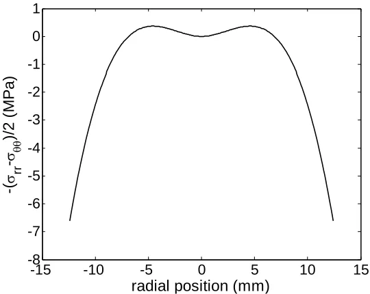
The difference between stresses, σ_rrf −σ_θθf , and the shear stress, σ_rθf , are given by

(

)

(

)

⎪ ⎪ ⎪ ⎪ ⎪ ⎪ ⎪ ⎭ ⎪ ⎪ ⎪ ⎪ ⎪ ⎪ ⎪ ⎬ ⎫ ⎪ ⎪ ⎪ ⎪ ⎪ ⎪ ⎪ ⎩ ⎪ ⎪ ⎪ ⎪ ⎪ ⎪ ⎪ ⎨ ⎧ ⎟ ⎟ ⎟ ⎟ ⎟ ⎠ ⎞ ⎜ ⎜ ⎜ ⎜ ⎜ ⎝ ⎛ + ⎥ ⎦ ⎤ ⎢ ⎣ ⎡ − − + + − ⎟⎟ ⎠ ⎞ ⎜⎜ ⎝ ⎛ + − − ⎟⎟ ⎠ ⎞ ⎜⎜ ⎝ ⎛ + + − − − − = −

∑

∫

∫

∑

∫

∫

∑

∫

∫

∫

∞ = ₊ + − − + ∞ = − − − ∞ = + + + 1 0 1 0 1 2 2 2 1 1 1 2 1 0 1 0 1 2 0 0 2 2 2 ) ( sin ) ( cos 1 1 3 ) ( sin ) ( cos 1 ) ( sin ) ( cos 1 ) ( 2 * 1 1 4

n R _n

19

(

)

(

)

⎪ ⎪ ⎪ ⎪ ⎪ ⎪ ⎪ ⎭ ⎪ ⎪ ⎪ ⎪ ⎪ ⎪ ⎪ ⎬ ⎫ ⎪ ⎪ ⎪ ⎪ ⎪ ⎪ ⎪ ⎩ ⎪ ⎪ ⎪ ⎪ ⎪ ⎪ ⎪ ⎨ ⎧ ⎟ ⎟ ⎟ ⎟ ⎟ ⎠ ⎞ ⎜ ⎜ ⎜ ⎜ ⎜ ⎝ ⎛ − ⎥ ⎦ ⎤ ⎢ ⎣ ⎡ − − + + + ⎟⎟ ⎠ ⎞ ⎜⎜ ⎝ ⎛ − − + ⎟⎟ ⎠ ⎞ ⎜⎜ ⎝ ⎛ − + − − − =

∑

∫

∫

∑

∫

∫

∑

_∫

_∫

∞ = ₊ + − − + ∞ = − − − ∞ = + + + 1 0 1 0 1 2 2 2 1 1 1 2 1 ₀ 1 0 1 2 2 2 ) ( cos ) ( sin 1 1 3 ) ( cos ) ( sin 1 ) ( cos ) ( sin 1 * 1 1 2

n R _n

s m f n R n c m f n n n n n n s s n R r n s m f n R r n c m f n n n r n s m f n r n c m f n n s s s f f f f r d h n d h n R r n R r n R n d h n d h n r n d h n d h n r n h E E E η ε η θ η ε η θ ν ν η ε η θ η ε η θ η ε η θ η ε η θ ν ν σ _θ .(1.23c)

Note that if the film thickness and misfit strain are uniform, the shear stress of Eq. 1.18 vanishes. Then the curvatures of Eqs. 1.22 become

0 , 1 1 6 2 = − − − = =

= _θθ ν ε κ _θ

ν κ

κ

κ _{m r}

s s s f f f rr h E h E , (1.24)

and the stresses in the thin film obtained from Eqs. 1.23 become

(

)

, 0

1− − =

= = = f r m f f f f rr f E θ

θθ _ν ε σ

σ σ

σ . (1.25)

For this special case only, both stress and curvature states become equibiaxial. The elimination of misfit strain ε_m from the above two equations yields a simple relation

(

ν

)

κ σ f s s s f h h E − = 1 6 2

, which is exactly the Stoney formula in Eq. 0.1.

20 both curvature and stress are related to the misfit strain distribution in Eqs. 1.22 - 1.23, so eliminating misfit strain from these equations will produce an extension to the Stoney formula.

The coefficients Cn and Sn related to the substrate curvatures are first defined by

(

)

(

)

sin ,

1 , cos 1 2 2

∫∫

∫∫

⎟ ⎠ ⎞ ⎜ ⎝ ⎛ + = ⎟ ⎠ ⎞ ⎜ ⎝ ⎛ + = A n rr n A n rr n dA n R R S dA n R R C ϕ η κ κ π ϕ η κ κ π θθ θθ (1.26)

where the integration is over the entire area A of the thin film, and dA=ηdηdϕ. Since both the substrate curvatures and film stresses depend on the misfit strain εm and film

thickness hf, elimination of these parameters gives the film stress in terms of substrate

curvatures as

(

)

(

)

(

)

(

)

, sin cos 1 1 4 ) 1 ( 6 1 2 ⎪ ⎭ ⎪ ⎬ ⎫ ⎪ ⎩ ⎪ ⎨ ⎧ + ⎥ ⎥ ⎦ ⎤ ⎢ ⎢ ⎣ ⎡ ⎟ ⎠ ⎞ ⎜ ⎝ ⎛ − − ⎟ ⎠ ⎞ ⎜ ⎝ ⎛ + − − + − = −

∑

∞ = − n n n n n rr f s f f f rr n S n C R r n R r n n h E θ θ κ κ ν σ σ θθ θθ (1.27a)

(

1

)

(

1

)

(

sin cos

)

,

2 1 4 ) 1 ( 6 1 2 ⎪⎭ ⎪ ⎬ ⎫ ⎪⎩ ⎪ ⎨ ⎧ − ⎥ ⎥ ⎦ ⎤ ⎢ ⎢ ⎣ ⎡ ⎟ ⎠ ⎞ ⎜ ⎝ ⎛ − − ⎟ ⎠ ⎞ ⎜ ⎝ ⎛ + + + − =

∑

∞ = − n n n n n r f s f f

r C n S n

R r n R r n n h E θ θ κ ν

σ _{θ θ}

(1.27b)

(

)

(

1

)

(

cos sin

)

,

1 1 1 1 ) 1 ( 6 1 2 ⎥ ⎥ ⎥ ⎥ ⎥ ⎦ ⎤ ⎢ ⎢ ⎢ ⎢ ⎢ ⎣ ⎡ + ⎟ ⎠ ⎞ ⎜ ⎝ ⎛ + + − − + − + + − + + − = +

∑

∞ = n n n n s s rr rr s s rr s f s s f f rr n S n C R r n h h E θ θ ν ν κ κ κ κ ν ν κ κ ν σ σ θθ θθ θθ

21 where κ +κθθ = 0 =

∫∫

(

κ +κθθ

)

/πR2

A rr

rr C dA is the average curvature over the entire

area A of the thin film, and Cn and Sn are given in Eq. 1.26. Equations 1.27, which

directly relate film stress to substrate curvatures, are known as the HR relations. It is important to note that stresses at a point in the thin film depend not only on curvatures at the same point (local dependence), but also on the curvatures in the entire substrate (non-local dependence) via the coefficients Cn and Sn. It should also be noted that Eq. 1.27b

for shear stress σ_rθf and Eq. 1.27a for the difference in normal stresses σ_rrf −σ_θθf are independent of the thin film thickness hf, but Eq. 1.27c for the sum or normal stresses

f f rr σθθ

σ + is inversely proportional to the local film thickness hf at the same point.

The interface shear stresses τ_r and τ_θ are also directly related to substrate curvatures via

(

)

(

)

(

)(

)

⎥⎥_⎦ ⎤ ⎢ ⎢ ⎣ ⎡ ⎟ ⎠ ⎞ ⎜ ⎝ ⎛ + + − − + ∂ ∂ − =

∑

∞ = − 1 1 2 2 sin cos 1 2 1 1 6 n n n n s rr s s s r R r n S n C n n R r h

E _{κ κ} ν _{θ θ}

ν

τ _θθ ,

(

)

(

)

(

)(

)

⎥⎥_⎦ ⎤ ⎢ ⎢ ⎣ ⎡ ⎟ ⎠ ⎞ ⎜ ⎝ ⎛ − + − + + ∂ ∂ − =

∑

∞ = − 1 1 2 2 cos sin 1 2 1 1 1 6 n n n n s rr s s s R r n S n C n n R r h

E _{κ κ} ν _{θ θ}

θ ν

τ_{θ θθ} ,

(1.28)

which is also independent of the film thickness hf. Equation 1.28 provides a way to

estimate the interface shear stresses from the gradients of substrate curvatures. It also displays a non-local dependence via the coefficients Cn and Sn.

22 significance. It shows that such stresses are related to the gradients of κrr +κ_θθ and not

to its magnitude as might have been expected of a local, Stoney-like formulation. Equation 1.28 provides an easy way of inferring these special interfacial shear stresses once the full-field curvature information is available. As a result, the methodology also provides a way to evaluate the risk of and to mitigate such important forms of failure. It should be noted that for the special case of spatially constant curvatures, the interfacial shear stresses vanish as is the case for all Stoney-like formulations described in the introduction.

The HR relations (Eq. 1.27) show a non-local dependence of film stress on

substrate curvature, that is, when a non-uniform misfit strain distribution exists, the stress as a given point is related to not just the curvature at that point but also the difference between that curvature and the average curvature across the wafer. The presence of non-local contributions in these relations has implications regarding the nature of diagnostic methods needed to perform wafer-level film stress measurements. In the presence of non-uniform curvatures, a local curvature measurement, i.e., a measurement at a single point, simply does not provide sufficient information to determine the local stress, i.e., the stress at that point. The existence of non-local terms in these relations necessitates the use of full-field methods capable of measuring curvature components over the entire surface of the plate system (or wafer). Furthermore, measurement of all independent components of the curvature field is necessary because the stress state at a point depends on curvature contributions (κrr, κθθ, and κrθ) from the entire plate surface.

23 arbitrarily non-uniform film thickness, the stress-curvature relations are identical to their counterparts for uniform film thickness [16, 17] except that thickness is replaced by its local value.

Axisymmetric HR Relations

In this section, the HR relations (Eq. 1.27) are simplified for a radially symmetric misfit strain [15]. The axisymmetric case is considered because the deformation of actual thin film-substrate systems often has radial symmetry, which implies a radially

symmetric misfit strain. This is partially due to the circular wafers, and partially to the axisymmetric effects from many of the processing steps, such as heating and cooling processes. A full-field curvature measurement of a typical 300 mm patterned wafer, which illustrates its axisymmetry, is shown in Fig. 1-2.

Figure 1-2. Principal curvature, κmax. This curvature is axisymmetric, implying that the deformation is

also radially symmetric.

24 Since a radially symmetric misfit strain has no θ terms, the Fourier series expansion of

Eq. 1.21 reduces directly back to hfεm: the leading term ( )

( )

/(2 )

2 0 0

∫

= π ε θ π

ε r h d

h_{f m c f m} is

m f

h ε , while the ( ε )

( )

2π ε cos θ θ/π 0

∫

= h n d

r

h_{f m} n_{c f m} and

( )

ε θ θ π

ε ) π sin /

( 2

0

∫

= h n d

r

h_{f m} n_{s f m} terms both vanish.

The curvatures of Eq. 1.22 then simplify to

⎥⎦ ⎤ ⎢⎣ ⎡ − ₋ + − − − = + ( ) 2 1 1 1

12 ₂ s _{m m}

m s s s f f f rr h E h E ε ε ν ε ν ν κ

κ _θθ ,

⎥⎦ ⎤ ⎢⎣ ⎡ ₋ − − − =

− ν ε

_∫

ηε η η

ν κ

κ _θθ d

r h E h E r m m s s s f f f

rr 2 2 ₀

2 ) ( 2 1 1

6 ,

0

= θ

κr , (1.29)

where ≡(2/ )

∫

( ) =

∫∫

/( 2)

0 2

R dA d

R R _{m m}

m ηε η η ε π

ε .

The stresses of Eq. 1.23 simplify to

) 2 (

1 _f m

f f f rr E ε ν σ

σ _θθ −

− = + , ⎥⎦ ⎤ ⎢⎣ ⎡ ₋ − − =

− ν ε

∫

ηε η η

ν σ

σ _θθ d

r h

E E

E _m r _m

s s s f f f f f

rr 2 ₀

2

2 ( )

2 1 1 4 , 0 = f rθ

σ . (1.30)

The coefficients Cn and Sn of Eq. 1.26 also vanish. Thus, the relations between

25 ) ( ) 1 ( 3 2 θθ

θθ _ν κ κ

σ σ − + − = − _rr f s f f f rr h E ,

[

]

⎭ ⎬ ⎫ ⎩ ⎨ ⎧ + − + + − + + + =

+ _{θθ θθ} κ κ_θθ κ κ_θθ

ν ν κ κ ν σ

σ _{rr rr}

s s rr f s s s f f rr h h E 1 1 ) 1 ( 6 2 , 0 = f rθ

σ , (1.31)

while the shear stress Eq. 1.28 simplifies to

) ( ) 1 ( 6 2 2 θθ κ κ ν τ + − = rr s s s r dr d h E , 0 = θ

τ . (1.32)

Note that there is still a non-local dependence of film stress on substrate curvature through the average curvature term κ_rr+κ_θθ .

Both the full HR relations (Eq. 1.27) and the axisymmetric, simplified HR relations (Eq. 1.31) will be used in this thesis.

An Analytical Example: Stoney vs. HR Relations

To illustrate the difference between the local Stoney formula and the new HR relations, consider a thin film-substrate system which is assumed to feature an out-of-plane displacement, w, due to some film stress, where

θ n R r w w n cos 0 ⎟ ⎠ ⎞ ⎜ ⎝ ⎛

= , (1.33)

w0 is the maximum displacement, and n is an integer. For n = 2, this displacement

26

(a) (b)

Figure 1-3. Wafer deformation from Eq. 1.33, where w0 = 20, n = 2, and R = 37.

Analytically, such a displacement gives curvatures of

(

)

θ κ

(

)

θ

κ

κ _{θθ θ} n

R r R w n n n

R r R w n n

n r

n

rr 1 cos , 1 sin

2 2

0 2

2 0

− −

⎟ ⎠ ⎞ ⎜ ⎝ ⎛ − − = ⎟

⎠ ⎞ ⎜ ⎝ ⎛ − = −

= , (1.34)

27

Since the radial and circumferential curvatures are equal and opposite, the localized Stoney formula (Eq. 1.1) predicts a vanishing stress state:

(

)

. 0

) 1 1 ( cos 1

) 1 ( 6

) (

) 1 ( 6

2 2

0 2

2

=

− × ⎟

⎠ ⎞ ⎜ ⎝ ⎛ − −

=

+ −

= +

−

θ ν

κ κ ν

σ

σ _{θθ θθ}

n R

r R w n n h h E

h h E

n

f s

s s

rr f s

s s f

f rr

(1.35)

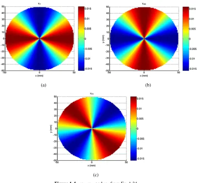
The HR relations (Eq. 1.27), however, infer stresses that do not vanish and are given by

(a) (b)

[image:34.612.126.533.71.449.2]

(c)

28

(

ν

)

(

)

θ

σ

σ _θθ n

R r R w n n h

E n

f s f f

f

rr 1 cos

1 3

2 2

2 0 )

( ) (

− ⎟ ⎠ ⎞ ⎜ ⎝ ⎛ − +

− = −

= , (1.36)

( )

(

ν

)

(

)

θ

σ _θ n

R r R w n n h

E n

f s f f

r 1 sin

1 3

2 2

2 0

− ⎟ ⎠ ⎞ ⎜ ⎝ ⎛ − +

= . (1.37)

These stresses are pictured in Fig. 1-5.

(a) (b)

[image:35.612.120.536.72.579.2]

(c)

Figure 1-5. Radial, circumferential and twist curvature from Eqs. 1.36 and 1.37.

30

2. Measuring Stress: X-ray Microdiffraction (

µ

XRD)

In order to determine the relative validity of the "nonlocal” stress/curvature relations compared to the "local" Stoney formula, it is necessary to employ a technique which is able to independently measure both the film stress and the substrate curvature at the same place on a wafer. The curvature can be used to calculate film stress using both types of relations (local and nonlocal), and the resulting stresses can be compared. The stresses from curvature can also be compared with the stresses determined from the direct measurement. The various implementations of X-ray microdiffraction (µXRD) provide such an opportunity. In general, X-ray diffraction (XRD) measures the crystalline lattice spacing in a material and uses the spacing change as a strain gage. Following the strain measurement, a constitutive law is used to infer stress in the film. In this particular project, synchrotron X-ray microdiffraction was used for these measurements.

Synchrotron µXRD has several advantages over traditional lab X-rays. These advantages include higher flux, smaller spot size, and the ability to quickly change between a

31

X-ray Diffraction: An Overview

In its most basic form, X-ray diffraction consists of an X-ray beam that is shined onto a specimen and then bounces off, diffracted by the specimen's crystalline lattice (Fig. 2-1). The resulting diffraction pattern, known as a Laue pattern, is captured with a detector. Within this basic framework the specifics of specimen, beam characteristics, and detector size can vary widely. The diffraction process is governed by the well-known Bragg's Law, d = λ / 2sinθ, which relates the incoming wavelength to the lattice spacing and diffraction angle. In this equation, λ is the beam wavelength, d the lattice spacing, and θ the angle between the beam and the plane of interest.

Figure 2-1. X-ray diffraction schematic

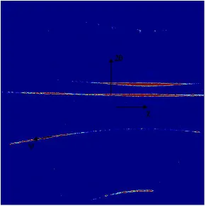
The diffracted beam forms Laue patterns, which are captured easily when using an area detector. Polychromatic diffraction patterns are composed of spots of high intensity (Fig. 2-2a), while monochromatic diffraction patterns, known as Debye rings, consist of high-intensity rings (Fig. 2-2b).

d

diffracted beam incoming

beam, λ

32

(a) (b)

Figure 2-2. Diffraction patterns from (a) white and (b) monochromatic incoming beams.

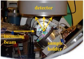
In a typical experiment, the specimen is held at a known angle to the incoming beam so that the area detector is able to capture as much of the diffracted beam as possible (Fig. 2-3). The resulting patterns are analyzed to obtain the desired

measurement at that location on the specimen. The specimen is translated across the beam in x and y so that a map is obtained, with images (or datapoints) taken at some specified spacing in x and y. For example, a line scan might have 10 datapoints spaced 0.1mm apart in x, while an area scan might have 5 of these x-lines spaced 0.5mm apart in

y. In this case the total area covered in the line scan is 1mm, and in the area scan is 2.5mm2. There are 50 images captured, so after analysis there will be 50 measurements across the sample surface (note: these are arbitrary numbers for illustrative purposes only.)

sample holder incoming

beam

[image:39.612.252.394.556.656.2]

detector

33 This is a pointwise measurement, which scans over the area of interest but does not get information from the entire surface. Also, it is important to note that the monochromatic and white beam measurements, though performed using the same

experimental setup, use different portions of the incoming X-ray beam and are effectively independent measurements.

Monochromatic µXRD

Monochromatic XRD uses a beam that is a single wavelength and diffracts into patterns called Debye rings. Each ring on the pattern is made up of many spots, and corresponds to a single lattice plane. Each spot corresponds to a single grain, but not every grain illuminated in the beam contributes to the diffraction pattern. Only the subset of grains that are oriented properly, namely whose specific lattice planes are at an angle to the incoming beam which corresponds to Bragg's law, will interact with the beam in such a way that it diffracts off of the crystal and impacts the area detector to create a spot. Therefore, in order to obtain well-populated rings, this technique works best when the grain size is much smaller than the beam spot size so that a large number of grains are illuminated at each point.

The average equibiaxial stress in the specimen (e.g., a thin film on some

[image:41.612.179.470.71.361.2]

34

Figure 2-4. Monochromatic pattern with coordinate system

The relevant equation for the d vs sin2ψ analysis as shown here is for equibiaxial stress (i.e., σxx = σyy = σ, σxy = 0).

σ ν ψ σ ν

E E

d d

d 2

sin

1 2

0

0 = + −

−

(2.1)

This stress is related to the lattice strain (d - d0)/d0 via the isotropic version of

Hooke's law. Constitutive isotropy is indeed a very good assumption for certain

polycrystalline films. For example, W, which is used in the present study, was chosen for its isotropic properties. Linear elasticity is also a good assumption for a material such as W, since its yield stress is very high compared to most commonly used metallic thin film materials.

To find the stress, a plot of d vs. sin2ψ is obtained (thus the technique's name). The lattice spacing, d, can be obtained from 2θ via Bragg's Law. To find 2θ, the rings are

2θ

χ

35 divided into small compartments of 2θ vs. ψ in a process known as binning. In each bin,

i, the intensity is integrated and fit to a Lorentzian function to find 2θ at maximum

intensity, or 2θi. Also, the average ψ for a bin, ψi, is found as ψi =(ψ_max +ψ_min )/2. Assuming the material constants are known, the other variable in this equation that must be determined in order to complete the analysis is d0, or the unstressed lattice

spacing. In practice, it is almost impossible to obtain this value, and the value at ψ = 0 is substituted. This is allowable because elastic strains introduce, at most, a 0.1%

difference between the true d0 and the d at any ψ. Since d0 is a multiplier to the slope, the

total error introduced by this assumption is less than 0.1% and is negligible compared to error from other sources [18].

To determine d0, ψi vs. 2θi is plotted and fit to a function (Fig. 2-5). Then 2θ is

found at ψ = 0, and d0 is calculated using Bragg's Law.

-40 -35 -30 -25 -20 -15 -10 73.62

73.64 73.66 73.68 73.7 73.72 73.74 73.76 73.78

ψ

2

θ

-0.0006x2-0.0150x+73.5096

36

0 0.1 0.2 0.3 0.4

1.291 1.2915 1.292 1.2925 1.293 1.2935

sin2(ψ)

d

-0.0051x+1.2933

Figure 2-6. plot of d vs sin2ψ

Finally the plot of d vs. sin2ψ is obtained (Fig. 2-6). For a truly equibiaxial stress state, the plot should be linear. A linear trend line is fit to the data, and by comparing the equation of that line with Eq. 2.1, the stress is easily found as

0 ) 1

( d

Es

ν σ

+

= , (2.2)

where s is the slope of the linear fit.

If the stress is not strictly equibiaxial, then this process determines the mean stress, or σ = (σxx + σyy)/2. For a complete analysis, this procedure is performed for each

37

Polychromatic (White Beam) µXRD

A polychromatic, or white, beam incorporates a range of wavelengths into the incoming light. In this case, the Laue patterns consist of many high-intensity spots (Fig. 2-7a). Each spot corresponds to a given lattice plane in a given grain. For a single grain of a known material, a known pattern of spots will be diffracted. If the grain is strained, the pattern shifts in a predictable manner. When there are several grains illuminated, the pattern for each grain is superimposed on the image. A sophisticated software program deconvolutes these images and indexes them, identifying individual patterns from each grain [19]. The software calculates the orientation matrix for each grain, as well as the deviatoric strain tensor in that grain. (The deviatoric stress is then found using Hooke’s law [18].) This technique is used when very few grains are in the illuminated region, since if there are too many superimposed patterns it becomes impossible for even the software to match the individual spots with the specific grain that produced them.

In the case of a single crystal specimen, the orientation matrix that is measured is always from the same grain. Once the crystal orientation is obtained at each location across the specimen, the relative slope and curvature are then determined by tracking the

(a)

α

sample normal

x, lab

y, lab

sample surface sample normal

projection in

xzplane

z, lab

(b)

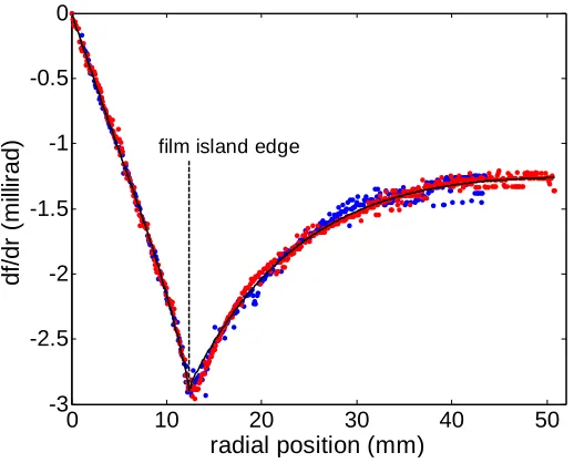
38 changes in the vector defining the grain normal with respect to the lab coordinate system. For a scan along the x axis (sample diameter), we are only concerned with the slope changes in the xz plane. This slope is equal to tan(α), where α is defined as the angle between the projection of the grain normal in the xz plane and the z axis in the lab reference frame (Fig. 2-7b).

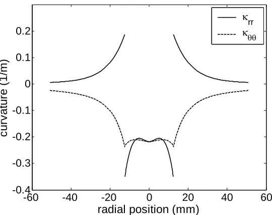
For a radially symmetric sample on which the scan is performed along the diameter, where y = 0, cylindrical coordinates can be used. The radial slope, ∂f/∂r = tan(α), and the circumferential curvatures κrr and κθθ are then determined from

r r

f rr

∂ ∂ = ∂ ∂

≡ 2₂ (tanα)

κ , (2.3)

) (tan 1

1 _α

κ_θθ

r r f r ∂ =

∂

39

3. Verifying Nonlocal Formulas: Comparison with XRD

In order to begin to verify the new analytical relations which allow for the

inference of film stress from nonlocal curvature measurements (nonlocal relations), the

two different types of µXRD measurements described in Chapter 2 were used to measure

both substrate slope and film stress across the diameter of an axisymmetric thin

film-substrate specimen composed of a circular W film island deposited in the center of a

single-crystal Si substrate [20]. The substrate slopes, measured by polychromatic (white

beam) µXRD, were used to calculate curvature fields and to thus infer the film stress

distribution using both the "local" Stoney formula and the new, "nonlocal" HR relations.

The variable film thickness, which was independently measured, was also an input to the

HR relations. These stresses were then compared with the film stress calculated from

lattice distortions measured independently through monochromatic µXRD, to determine

the validity of the new formula and to quantify the improvement over the commonly

accepted Stoney analysis.

Methodology

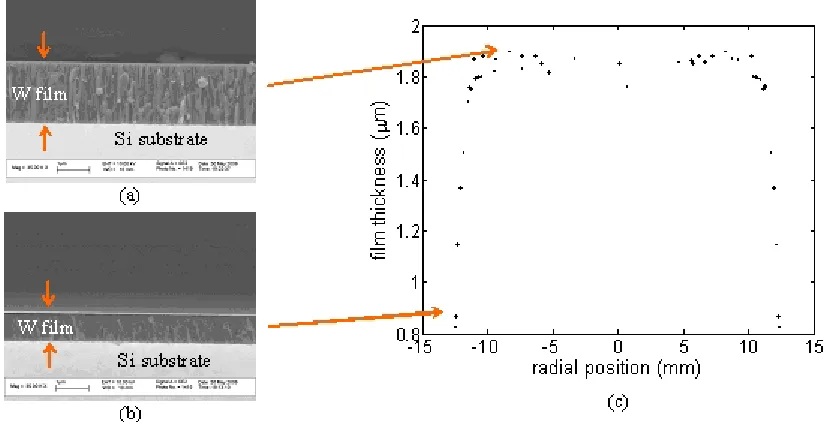
The specimen consisted of a circular, 24.8 mm diameter W film island deposited

on the center of a 100 mm diameter, 525 µm thick Si <001> wafer (Fig. 3-1). The film

thickness is variable across the island; the thickest portion, in the center of the island, is

approximately 1.85 µm. The Young’s modulus for Si and W are 130 GPa and 410 GPa,