Population coding and reconstruction of complex stimuli in the locust olfactory system

Full text

(1)Population Coding and Reconstruction of Complex Stimuli in the Locust Olfactory System. Thesis by Bede Michael Broome. In Partial Fulfillment of the Requirements For the Degree of Doctor of Philosophy. California Institute of Technology Pasadena, California 2006 (Defended January 6, 2006).

(2) ii. © 2006 Bede Michael Broome All Rights Reserved.

(3) iii. To my family and my love. Without you, this would never have been possible..

(4) iv. Acknowledgements Although the act of receiving a PhD is a singular achievement, the process of performing graduate research is a highly collaborative one. I would like to thank my advisor, Gilles Laurent, for his analytical and critical assessment of the material covered in this dissertation. His constant skepticism and methodical approach to understanding problems, without losing sight of the big picture, has affected me deeply. Also, I would like to thank my committee members: Michael Dickinson, Mark Konishi, Thanos Siapas, and Erin Schuman. Their suggestions and encouragement have guided me through the sometimes difficult process of finding a good research project and sticking to it. I would also like to thank the members of the Laurent Lab for endless hours of encouragement and assistance with everything from minute experimental details to my overall understanding of neuroscience. In particular, I would like to thank Vivek Jaramayan, who collaborated with me extensively on the work in chapter 2 and under whose guidance I have become far more knowledgeable about the principles of neural coding, Matlab programming, and data analysis. Also, I owe great thanks to a visiting member of our lab, Markus Meister. Markus’ sabbatical turned into a very productive collaboration and the contents of chapter 3. It was very interesting to learn about science from a different viewpoint, and his technical expertise was essential for developing the electronic nose and the stimulus protocols used with it. I would like to recognize the individuals whose early encouragement led me to pursue a career in science: Fernando Nottebohm, Edward Ziff, James Schwartz, Ashok Hegde, and Edward Vates. I owe particular thanks to Ed for getting me interested in research at an early age and for providing such a good career model. I am extremely appreciative of the help I have received from my friends and family, and I am eternally indebted to my parents for their love and encouragement throughout medical and graduate school. Finally, I would like to thank my best friend Oceana Blueskyes, my partner in life, for her unwavering support throughout my PhD years. Her love and companionship have provided me with the stability both in body and mind that were necessary for completing this degree..

(5) v. Abstract Odors evoke complex sequences of activity in antennal lobe projection neurons (PNs), the insect analogs of mitral/tufted cells. These PN activity patterns evolve over hundreds of milliseconds, are consistent across trials, and contain information about odor identity and concentration. However, in natural settings animals must often identify odor blends or multiple odorants that occur in short temporal succession. We explored the effects of such stimulus history on single cell PN activity, PN ensemble responses, and downstream Kenyon cell (KC) responses by performing two experiments with novel stimulus paradigms. In the first experiment two different odors with variable intervening delays were presented while recording from PN and KC ensembles in the locust. We found that PN ensemble representations rapidly tracked odor stimulus changes and, in conditions of temporary odor overlap, often corresponded to the representation of neither odor alone nor their binary mixture. KC responses tracked the specificity of the instantaneous state of the PN representation: for example, for stimulus conditions that lead to unique and unpredictable PN population activity, we could find KCs with correspondingly unique spiking. These results support the hypotheses that PN population dynamics are history dependent and that PN output is read broadly in space (over the PN population) and piecewise in time by its target population. In the second experiment two different odors were presented either as single pulses or complex M-sequence odor stimuli while we recorded PN activity and the time-varying stimulus using a specially adapted electronic sensor. Our results describe the numerous similarities between the processing of stimuli with diverse frequencies and highlight several important differences. We found that PN response types are varied, low dimensional, and that individual PNs do not fall into stable functional classes. Also, PN ensembles occupy different regions of high dimensional coding space and follow trajectories that depend on stimulus history. Finally, an observer’s ability to reconstruct either the concentration or identity of an odor improves with PN number. These results add support to a growing body of evidence that Kenyon cells, the targets of PNs in the mushroom bodies, carry out a pattern classification on PN activity vectors sampled over large sets of PNs..

(6) vi. Table of Contents. Acknowledgements. iv. Abstract. v. Table of Contents. vii. 1 Introduction. 1. 1.1 Neural Coding. 2. 1.2 Insect Olfactory Anatomy. 6. 1.3 Olfactory Coding in the Locust. 12. 1.4 Decoding Neuronal Activity. 15. 1.4.1 Population Vector Coding. 16. 1.4.2 Bayesian Inference. 18. 1.4.3 Spike-Train Decoding. 21. 1.5 Outline. 2 Encoding and Decoding of Overlapping Odor Sequences. 22. 25. 2.1 Introduction. 25. 2.2 Results. 27. 2.2.1 PN Responses to Overlapping Odor Patterns. 27. 2.2.2 Single PN Responses to Overlapping Odor Pulses. 29. 2.2.3 PN Population Responses to Overlapping Odor Pulses. 32. 2.2.4 Decoding of PN Trajectories by Kenyon Cells. 40. 2.3 Discussion 2.3.1 Temporal and Spatial Scales of Analysis. 48 49.

(7) vii 2.3.2 Importance of Stimulation History. 50. 2.3.3 Possible Mechanisms. 52. 2.3.4 Consequences for Natural Odor Plume Conditions. 54. 2.4 Methods. 55. 2.4.1 Odorants. 55. 2.4.2 Electrophysiology. 55. 2.4.3 Data Analysis. 57. 2.5 Acknowledgements. 59. 3 Encoding and Reconstructing Rapidly Varying Odor Stimuli. 60. 3.1 Introduction. 60. 3.2 Results. 62. 3.2.1 Electronic Nose. 62. 3.2.2 Single PN Responses. 65. 3.2.3 Functional Subdivisions within the PN Population. 69. 3.2.4 PN Trajectories Corresponding to Rapidly Varying Stimuli. 73. 3.2.5 Reconstructing Odor Concentration Profiles. 78. 3.2.6 Reconstructing Odor Identity Profiles. 80. 3.3 Discussion. 86. 3.3.1 Stimulus Structure and PN Properties. 86. 3.3.2 Are There PN Classes?. 88. 3.3.3 Rapidly Varying Stimuli vs. Single Pulses. 90. 3.3.4 How Many PNs Should Their Decoders Sample?. 92. 3.4 Methods. 94. 3.4.1 Odorants. 95. 3.4.2 Electronic Nose. 95. 3.4.3 Electrophysiology. 95. 3.4.4 Data Analysis. 96. 3.4.5 Calculating and Comparing ST-SAs. 97. 3.5 Acknowledgements 4 Concluding Remarks. 98 99. 4.1 Summary of Results. 99. 4.2 Significance of Results. 102. 4.3 Future Directions. 104. References. 106.

(8) 1. Chapter 1. Introduction. “Last of all he will be able to see the sun, and not mere reflections of him in the water, but he will see him in his own proper place, and not in another; and he will contemplate him as he is.” -Plato, The Republic, The Allegory of the Cave. The process by which sensory events transform into subjective experiences is a matter of great mystery and inquiry. First, the brain receives information through specially tuned receptors, each with their own properties and sensitivities. Then, the output of these sensors is conveyed to other brain regions, transformed, and processed so that representations (platonic shadows) of the outside world are formed within our minds. Thus, the richness that we see, hear, feel, taste, and smell in the outside world is in fact both a filtered and a rebuilt version of reality. We will never escape our cave, the internally reconstructed version of the world around us. The representations that we form are fundamentally based upon and constrained by the complex rules that govern our cellular biology, our systems level interactions, and the world around us. Understanding how the brain forms these representations is critical for appreciating the human experience. In this thesis I will address several issues related to the formation of odor representations in the insect olfactory system. By elaborating on the mechanisms behind the neural coding processes that drive these constructs, I hope to bring new understanding to the principles that underlie our perceptions of the world around us..

(9) 2. 1.1 Neural Coding To understand how the brain forms representations of sensory events, we must first decipher the language that the brain uses to encode information. At a basic level, all neural systems employ similar biochemical/electrical mechanisms to generate and propagate information. Electro-chemical gradients across neuronal membranes give rise to action potentials (“spikes”) when input to gating mechanisms within the membrane exceed threshold voltages as a result of external stimuli (Bernstein, 1902; Hodgkin and Huxley, 1952). These spikes travel the length of the neuron and stimulate the release of pooled neurotransmitters at the synapse (Eccles, 1976; Loewi and Navratil, 1926). This, in turn, activates downstream neurons. Variations in either the anatomical organization of the cells or the mechanisms related to spike generation/propagation act as mechanisms to store information and adapt to the outside environment (Kandel et al., 2000). At the periphery, single neurons in a sensory system detect some form of energy (e.g., a photon, or kinetic energy) or chemicals (in the case of taste and olfaction) and transform those into electrical signals. Those signals are transmitted to and received by other neurons, and thus, they become the carriers of information about the physical world. For example, each photoreceptor captures photons of specific spectral quality and intensity in some volume of space. Collectively, photoreceptors provide signals from which a visual field can be constructed, even though each neuron “encodes” only a very small portion of that space. However, as those signals proceed from the periphery, they are combined in complex ways, and functionally relevant features are extracted. The mammalian visual system provides a clear example of this progression (Gilbert, 1994; Lagnado and Baylor, 1992; Reid and Alonso, 1996). As signals from photoreceptors proceed to further layers of the retina and ultimately to ganglion cells, information about constructed features —edges, concentric light/dark regions, wavelength—can be found in the activity of single neurons. Such information is often said to be explicit. The same information.

(10) 3 is of course present, implicitly, in the collective activity of arrays of upstream neurons. Of particular interest is the recent realization that such features match the statistical structure of our physical world (Yang and Purves, 2003). From the retina, signals are conveyed to the lateral geniculate nucleus in the thalamus and then on to the visual cortex, where we find, for example, neurons sensitive to orientation, motion, and color (Livingstone and Hubel, 1988; Sincich and Horton, 2005). As individual neuronal responses become more specific or selective, it is obvious that a reconstruction of the world that matches our perception must require the pooling of activity from many neurons. Therefore, information is said to be distributed (Callaway, 2004; Martin, 2002). How do brain networks process and use distributed signals? Different types of “coding” strategies can be found in neural systems; at one extreme are what are often called spatial representations (Rieke et al., 1997). Those can in turn be split into identity codes and truly spatial codes—i.e., ones in which neuronal position is intrinsically relevant for the encoding or decoding mechanisms. The encoding of spatial position by the retinal array of photoreceptors, or the encoding of spatial position by delay lines in the owl’s nucleus laminaris (Konishi, 2003; Meister, 1996), for example, are true spatial codes. At the other extreme are “temporal codes” (Laurent, 1999). These can also be split according to whether the codes are representations of time or temporal encoding of features that do not, in and of themselves, vary in time. The latter are considered true temporal encoding schemes. These schemes are not necessarily exclusive of one another; they can often be superimposed depending on a system’s specific requirements (Ahissar and Arieli, 2001). They are also to a significant extent dependent on the metrics used to characterize neuronal activity. For example, a temporal code is nearly always also an identity code simply because the identities of the neurons whose firing carries information are themselves informative. In addition, the information present in the timing of a population’s spikes disappears as one uses longer and longer time windows to quantify it: essentially, a potentially temporal representation becomes a spatial one as one measures rates over long time periods. This reveals.

(11) 4 that the nature of a code depends on the prior knowledge of the mechanisms by which this information is normally decoded. Time codes do not depend on a cell’s location but rather its activity. Within time coding a distinction is often made between rate codes and temporal codes. Again these two descriptions are not exclusive, but rather two ends of a spectrum (Shadlen and Newsome, 1994). A pure rate code conveys information using only the mean firing rate of its spikes (Parker and Newsome, 1998; Sanger, 2003). Early pioneers in neural coding discovered the first example of such a system while recording from mechano-sensitive stretch receptors, finding that stretch was directly proportional to the mean spike rate (Adrian, 1942). In contrast, a pure temporal code does not depend on the intensity of a particular spike burst but on the precise timing of spikes relative to one another (Shadlen and Newsome, 1994; Theunissen and Miller, 1995). While theories about neuronal coding date back to the experiments of Lord Adrian in the 1930’s, our understanding of temporal coding has, until recently, been quite spare. Perhaps the main reason for the relative dominance of rate coding in our models of the brain (in all but a few specialized cases) has been our inability to record from large sets of neurons (Nicolelis et al., 2003; Nicolelis and Ribeiro, 2002; Wilson and McNaughton, 1993; Wilson and McNaughton, 1994). While rate codes can be understood by monitoring the activity of a single cell, temporal codes often require the ability to monitor the responses of many cells simultaneously (Buzsaki, 2004; Deadwyler and Hampson, 1997). Thus, temporal coding has been studied relatively less than rate coding, but it is no less significant. In fact, temporal coding is a particularly attractive way for information-rich signals to be processed. It could, for example, enable neurons to bind together their activity, working in parallel to represent information (Engel et al., 2001; Engel and Singer, 2001). Individual processing capabilities may be combined when groups of neurons project onto the same downstream target that acts as a coincidence detector. Each of the input neurons acts to bring the downstream neuron closer to threshold, summating their input (Dayan and Abbott, 2001; König.

(12) 5 et al., 1996). For larger groups temporal coding can be used to organize activity through synchronous oscillations. In this situation neurons fire in time with an internally or externally (with respect to a specific brain region) generated synchronizing mechanism, and all of the information from one cycle is linked together by nature of its timing (Singer, 1999; Singer, 1995). Synchronized oscillations of this type have been observed across many different phyla. These include: primates - gamma oscillations (30-90Hz) have been linked to such diverse processes as attention (Fell et al., 2003; Tiesinga et al., 2004) and memory (Lee et al., 2005; Mehta, 2005); rodents - theta oscillations have been linked to hippocampal activity (Siapas et al., 2005; Siapas and Wilson, 1998); amphibians – oscillations are used to increase information transmission in the retina (Schnitzer and Meister, 2003); crustaceans – oscillations have been found to regulate activity in the stomatogastric ganglion (Bartos et al., 1999; Marder, 2002); and arthropods – oscillations are necessary for fine olfactory discrimination (Stopfer et al., 1997). However, coincidence detection and oscillatory activity are not the only ways in which temporal coding can be used in the brain. Rank order coding is a strategy where the timing of a cell’s first spike carries significance. This method has been demonstrated to be an efficient means for representing information both experimentally and theoretically in the visual system (Delorme and Thorpe, 2001; Thorpe et al., 2001; Van Rullen et al., 1998). In this model downstream neurons are very sensitive to the activation order of inputs by a feed-forward shunting mechanism that progressively reduces the sensitivity of the downstream neuron to its inputs. Investigations into this method of coding are ongoing. Finally, neurons can organize themselves into so-called synfire chains - systems capable of generating repeating patterns in response to a stimulus trigger (Ables, 1991; Aviel, 2003). To achieve this state, neurons are connected so that once activated groups of synchronously firing neurons will activate one another in a self-perpetuating manner. These many observations of complex structure in neuronal activity suggest a diversity of potential coding mechanisms in the brain. The hard part is to establish their functional relevance..

(13) 6. 1.2 Insect Olfactory Anatomy Animals are constantly bombarded with an enormous number of odors. The powerful ability of the olfactory system to detect and discriminate between these odorants allows animals to perform some of the most essential tasks for their survival: find food, find mates, and avoid predators. Olfaction is the oldest, most conserved sense, and many of its mechanisms are identical across phyla. For example, convergent anatomy, recurrent interactions, serial processing, and oscillatory activity have all been observed in both insects and mammals (Firestein, 2001; Hughes and Mazurowski, 1962; Laurent and Naraghi, 1994; Mombaerts, 1996; Nicoll, 1971b.). The insect system’s similarity to the mammalian system, both structurally and functionally, enables one to probe the complexities of neural coding and use invasive techniques that would be difficult in larger organisms. Due to its smaller physical size, the insect is a far more tractable system. While in mammals the olfactory bulb contains four types of neurons and greater than one million cells, the insect antennal lobe contains only ~1000 neurons and two classes of cells (Firestein, 2001; Leitch and Laurent, 1996). This reduced complexity allows one to better understand the specific interactions that govern olfactory processing before testing these conclusions in mammals. Insects in general and the locust (Schistocerca americana) in particular have advantages for the study of olfaction. Insects are highly olfactory animals and can find both food sources and potential mates (despite poor visual acuity) over large habitats using olfactory cues. Accordingly, a relatively large portion of their brain is dedicated to olfaction, making these areas experimentally accessible. Also, insects are not simple creatures and have been shown to exhibit complex behaviors previously ascribed only to larger animals. These include: associative learning (Bitterman, 1983), complex decision-making (Giurfa, 2003; Giurfa et al., 2001), and navigation through landscapes (Srinivasan, 2003). Most recently, social learning, the transference of.

(14) 7 knowledge between individuals without outside instruction, has been demonstrated in crickets (Coolen et al., 2005). The fact that insects can accomplish such complex tasks allows us to investigate not only low level sensory systems but also higher level structures where information integration occurs and decisions are made.. Finally, there are several unique advantages. associated with locusts. They are large, easy to manipulate, capable of withstanding intrusive physiological recordings, and the subject of considerable prior physiological work (Burrows, 1996; Laurent, 1997). Also, locusts have certain populations of neurons whose anatomy and firing characteristics enable one to record the activity of specific large groups of neurons unambiguously (Perez-Orive et al., 2002). The overall organization of both the mammalian and insect olfactory systems is shallow; at each one of few relays, transformations occur and representations change. Olfactory stimuli are initially transduced by olfactory receptor neurons (ORNs). In locusts these are exclusively found on the antenna; however, in other insects they also appear on the maxillary palps or elsewhere (Chapman, 1998). In mammals these receptors are located in the olfactory epithelium within the nasal cavity. While mammalian ORNs have no structure enclosing them, insect ORNs, are located within small, porous protrusions of the cuticle called sensilla (Chapman, 1998; Keil, 1989; Steinbrecht, 1980). Each sensillum typically possesses two or more ORNs with some locust sensilla containing up to 50 ORNs (Keil, 1989; Ochieng et al., 1998). Sensilla come in four different types, of which three are known to contain ORNs. Each different type of sensilla (basiconic, trichoid, coeloconic, chaetic) occurs with a different frequency and in different regions of the antenna (Lee and Strausfeld, 1990). Among those sensilla that are known to contain ORNs, basiconic and coeloconic sensilla are most densely clustered at the proximal and middle regions of the antenna, while trichoid sensilla are located more distally. Little is known about the arrangement of individual receptors, in contrast with the extensive knowledge about the mammalian olfactory epithelium (Buck, 1991; Mombaerts, 1999; Scott and Brierley, 1999; Scott et al., 1997)..

(15) 8 Within the sensilla a wide variety of olfactory receptors (OR) bind with varying affinities to the large number of odorants encountered in nature (Hallem et al., 2004; Wilson et al., 2004). Work in round worms, insects (Drosophila and mosquitoes), and mammals (mice, dogs and humans) has uncovered several families of G-protein coupled receptor (GPCR) genes expressed in olfactory neurons. They form the largest gene super-family in the genome (Buck, 1991; Vosshall et al., 1999). In rats, an extreme case, ORs make up 6% of the genome, although many of these genes are non-functional pseudogenes. In Drosophila, 55 functional olfactory receptors have been identified, and in mammals approximately 1000 (~400 in humans, ~1400 in rats) are present (Couto et al., 2005; Hallem et al., 2004; Mombaerts, 1999; Vosshall et al., 2000). To date, there is no similar count of the unique ORNs types in locusts; however, we do know that there are 50,000-90,000 ORNs on each locust antenna (Burrows, 1996; Leitch and Laurent, 1996). ORNs arborize in glomeruli, roughly spherical regions of neuropil in the antennal lobe (AL), the insect equivalent of the mammalian olfactory bulb. Surprisingly, each Drosophila and mammalian ORN (this finding has yet to be replicated in other species) expresses only a single type of OR gene (2 in Drosophila, with one conferring binding specificity) from this large repertoire, and each ORN that shares the same OR projects to a single glomerulus (Mombaerts et al., 1996; Vosshall et al., 2000). This occurs regardless of the physical location of the ORN on the olfactory epithelium/antenna. Odorant molecules bind to ORs associated with one of the two pathways for odor transduction: cAMP and IP3. Odorant molecules that stimulate GPCRs cause them to activate GTP effectors that facilitate the production of cAMP. The rise in this intracellular second messenger causes a membrane bound cyclic-nucleotide gated Ca2+ channel to open, depolarizing the cell and giving rise to an action potential that carries the ORN’s information downstream (Ache and Young, 2005; Zufall and Leinders-Zufall, 1998). The other intracellular messaging pathway, the IP3 dependent pathway, has been molecularly identified primarily in crustaceans, but it is thought to exist in a diverse range of animals across phyla. In a similar fashion to the cAMP.

(16) 9 pathway, odor reception triggers IP3 production that then opens IP3 gated Ca2+ channels, depolarizing the cell and eliciting a spike (Ache and Young, 2005; Boekhoff et al., 1990). It is currently unknown whether individual ORNs use both pathways simultaneously or what the functional effect of a redundant system might be (Ache and Young, 2005; Takeuchi et al., 2003). In the locust, projections from ORNs travel ipsilaterally - in flies and mammals the projections are bilateral - to antennal lobe glomeruli (Hansson and Anton, 2000). There they synapse directly onto two different cell types: excitatory projection neurons (PNs) and inhibitory local neurons (LNs) (Fig. 1.1) (Ernst et al., 1977). Anatomical studies have demonstrated that in the locust there are 830 PNs and approximately 300 LNs (Leitch and Laurent, 1996). Cholinergic PNs extend dendrites to 10-14 coplanar glomeruli, equidistant from the center of the AL (R Jortner, SS Farivar, & G Laurent, in prep; Wehr and Laurent, 1999). The multiglomerular nature of locust PNs is relatively unique, having only been noted in locusts and wasps amongst the many species studied. Drosophila possess uniglomerular PNs, and honeybees have both uni- and multiglomerular PNs (Fonta et al., 1993; Homberg et al., 1988; Stocker et al., 1990). However, it is not known whether the multiglomerular PNs in locusts or bees all receive projections from the same OR, effectively making them uniglomerular systems. Projection neurons are the sole output neurons of the locust AL and project ipsilaterally to the calyx of the mushroom body and the lateral protocerebrum (Hansson and Anton, 2000). As with the PN inputs, the output pattern varies across different insect species. Drosophila and bee PNs do not all project to both destinations, and in contrast to the locust some PNs project only to the lateral protocerebrum (Jefferis et al., 2001; Wong et al., 2002). Locust LNs project broadly across the AL and form dendrodendritic, GABAergic synapses with a large number of the PNs (Fig. 1.1)(R Jortner, SS Farivar, & G Laurent, in prep; Hansson and Anton, 2000). While different classes of LNs have been observed, each defined by its projection pattern, all are densely arborizing cells whose neurites are completely limited to the AL. In addition, LNs are axonless and in the locust do not produce action potentials, enabling us.

(17) 10 to record from large groups of cells and unambiguously attribute the activity to PNs (Perez-Orive et al., 2002). LNs respond to odor stimuli with graded sub-threshold activity and calcium spikes (Laurent and Davidowitz, 1994; Leitch and Laurent, 1996). Just as with PNs, LNs are not identical in all insect species. In some insects systems (such as bees and cockroaches) LNs project only to limited portions of the AL, and in others they spike. However, they are consistently both inhibitory and GABAergic (Hansson and Anton, 2000; Homberg et al., 1989).. Figure 1.1 Anatomy of the locust olfactory system. A. Structures: AL - antennal lobe; AN antennal nerve; KC - Kenyon cell; LN - local neuron; LPL - Lateral protocerebral lobe (lateral horn); MB - mushroom body; PN - projection neuron. LN is shown as a cut out to demonstrate its broad branching throughout the AL. B. Actual anatomy of locust brain shown using an antiGABA stain. Figures adapted from Wehr & Laurent 1996 and Perez-Orive et al. 2002.. The mushroom body (MB) is a primary recipient of AL projections and is one of the integrative nexuses in the insect brain, receiving input from the visual, olfactory, and tactile sensory systems (Burrows, 1996; Gronenberg, 2001; Strausfeld et al., 1998). Projections from the AL follow the antennal tract to the calyx of the MB where they branch broadly throughout the MB calyx (Fig. 1.1). There are approximately 50,000 intrinsic neurons, termed Kenyon cells.

(18) 11 (KCs), in the locust MB (Laurent and Naraghi, 1994). These small cells (3-8µm) have cell bodies located above the calyx and send their primary neurites down into the calyx where their neurites divide and fan out, projecting over a small region (Laurent and Naraghi, 1994; R Jortner, SS Farivar, & G Laurent, in prep). A single PN makes contact with approximately 1/2 of all KCs and covers approximately 10% of the MB calyx (R Jortner, SS Farivar, & G Laurent, in prep). As with the other cell types in the olfactory system, there are inter-species differences with respect to KC organization. For example, bees, cockroaches, and wasps have two calyces per MB, while locusts and Drosophila possess only one (Strausfeld et al., 1998; Strausfeld et al., 2003). Kenyon cell axons all leave the MB via the pedunculus, a structure located at the base of the MB. These densely packed axons carry KC information to several different lobes. Locust KCs project to two lobes (the α- and β-lobes), while additional structures are present in other insects (α’-, β’-, and γ-lobes are present in Drosophila) (Strausfeld et al., 1998). In the lobes, KCs synapse onto MB extrinsic neurons that then project widely throughout the brain. While little is known about the anatomy or function of projections that follow after the MB, oscillations have been detected in their activity. Desynchronizing upstream PNs has been shown to decrease the specificity of their response, a result that has also been demonstrated in KCs (MacLeod et al., 1998). Further investigation into these downstream areas is ongoing. In comparison to the MB, relatively little is known about the structure and function of the lateral horn, the second output region of the AL (Hansson and Anton, 2000). In locusts, lateral horn interneurons (LHIs) are GABAergic cells that project directly to the MB. There, the profuse axon branches overlap with KC dendrites. Experiments have shown that LHIs respond to most odors, suggesting a role for them in the modulation of MB activity (Perez-Orive et al., 2002)..

(19) 12. 1.3 Olfactory Coding in the Locust While there is still much to discover about olfaction, a picture of how odors are represented at different points in the locust olfactory system has begun to emerge. Odors initially activate multiple odor receptors with varying affinities (Hallem et al., 2004; Wilson et al., 2004). This promiscuous activation, using sets of ORNs to represent an odor, allows locusts to perceive a virtually limitless number of odors. The alternative, where each odor activates only one specific receptor, would limit their perception to the number of different receptors on the antenna, ~1000. As the signal progresses to the AL there is a dramatic reduction in the number of cells that represent the odor information. The highly convergent nature of this connection (100,000 ORNs  800 PNs) is thought to reduce the significance of noise fluctuations on the odor signal in the AL (Laurent, 2002). Nonetheless, a very large fraction of PNs are activated by the ORNs. 90% of all PNs (in the locust) respond to the presence of an odor with either excitation (~50%) or inhibition (~40%) of their activity relative to their basal firing rate (Perez-Orive et al., 2002). This widespread activity appears to arise not only from the primary activation of the PNs by ORNs, but also by recurrent interactions within the AL (Leitch and Laurent, 1996; MacLeod and Laurent, 1996). It is notable that this activity does not occur only in specific regions, and odotopic mapping is not the primary means for representing information in the OB or AL (Laurent, 1999). Recordings of local field potentials (LFP) in the mushroom body calyx indicate that PN activity occurs in 20-30Hz oscillatory cycles when odors are present and that the power of these oscillations drops significantly when odors are removed (Laurent and Davidowitz, 1994; Laurent and Naraghi, 1994). It is believed that PNs use this synchronous firing to bind together the activity of numerous PNs and form a representation of each unique odor. Thus, it appears that odors are not represented by the momentary activity of a single PN or even a single PN pattern, but by 830 dimensional PN ensembles occurring at the rate of 20-30Hz (Mazor and Laurent, 2005). It has also been shown that these 830-D representations are not static repeating patterns,.

(20) 13 but patterns that evolve over time. Not all PNs fire in each oscillatory cycle; instead, PNs transiently synchronize their activity in ensembles that change over time and in an odor-specific manner (Laurent and Davidowitz, 1994; Laurent and Naraghi, 1994). A given PN that is highly synchronized with another PN for one cycle may be unsynchronized or silent in the next one. These evolving ensembles take advantage of the fact that odors are usually present for a prolonged period. As odor presentations continue, the ensembles that are activated become more and more dissimilar from one another. In zebrafish this decorrelation process was shown to reach its maximum in 200-300ms (Friedrich and Laurent, 2004), a time period that is consistent with rodent experiments as the point when discrimination between odors can be expected (Uchida and Mainen, 2003). This oscillatory synchronization is mediated by the recurrent activity between PNs and LNs in the AL. While LNs do not spike in locusts, their contribution to synchrony has nonetheless been demonstrated in two ways. First, LNs sub-threshold activity has been directly monitored using intracellular recordings, showing strict locking to LFP phases observed downstream (R Jortner, SS Farivar, & G Laurent, in prep). Second, selective blocking of GABA (primarily associated with LNs) in the AL has been shown to stop oscillations of the downstream LFP (which reflects the activity of the AL PNs) (MacLeod et al., 1998; MacLeod and Laurent, 1996; Stopfer et al., 1997). Others have suggested that lateral inhibition (in the strict visual system sense, where feedback from neighboring cells acts to sharpen the tuning curve of a particular cell in respect to a certain odor) is present in the AL and modulates PN activity (Mori et al., 1999). However, this hypothesis is unlikely given the widespread PN activity that is detected across both the OB and the AL in response to odors and the lack of traditional tuning curves in the AL. Behavioral evidence suggests that oscillatory synchronization of PNs is essential to an animal’s ability to perform fine discriminations between odors. Using honeybees, it was demonstrated that abolishing oscillations using the GABA blocker picrotoxin inhibited the ability.

(21) 14 of the animal to discriminate between similar single chain alcohols (1-hexanol and 1-octanol) (Stopfer et al., 1997). However, their ability to discriminate between dissimilar odorants (geraniol and 1-hexanol) was not disturbed. Similar oscillations have been found in all model organisms with the exception of Drosophila. However, the significance of oscillations in other systems has not been thoroughly examined. It is important to note that this distributed method of representing odors may not be used in all circumstances. One prominent exception may be the case of pheromones. Pheromones are compounds that are used for communication between individuals of a particular species for a wide variety of purposes including: mating, alarm transmission, territorial marking, and group aggregation. Animals are highly tuned to these compounds and may use special receptors or processing areas to ensure that these signals are correctly interpreted (Amrein, 2004; Brennan and Keverne, 2004; Hassanali et al., 2005). In moths specific glomeruli have been identified that mediate pheromone activation, and it appears that all the activity necessary to represent sex pheromones at the AL level is confined to within two specific glomeruli (Christensen and Hildebrand, 2002). This may represent an instance of labeled lines, single pathways used for information transmission, in the AL. While some have suggested that a system of labeled lines is used for all odor representations, there is significant evidence to dispute this hypothesis. First, odors cause widespread activation in the AL, something that would not be expected with labeled lines. Second, the diversity of odorants that an animal can recognize suggests that it is not limited by the relatively small number of pathways present in a labeled line model. Thus, while there may be some specialized odors for which labeled lines are useful, most odors are probably represented in the AL by distributed coding strategies. Until recently, the size and recording difficulty associated with the MB hampered our ability to investigate its function. The existing evidence for its function came mainly from genetic and developmental studies that demonstrated the MB’s involvement in learning and memory for both olfactory and visual information (Dubnau et al., 2001; McGuire et al., 2001; Strausfeld et al.,.

(22) 15 1998). More recent studies have begun to shine light on how the MB integrates olfactory information from incoming PN ensembles. Each KC responds to approximately 10% of the odors presented to it and does so with a few very tightly times spikes (Perez-Orive et al., 2002). This stands in stark contrast to the promiscuous and prolonged firing of PNs. KCs owe their specificity to their high firing thresholds, the highly divergent nature of the PNMB connection (83050,000), and the synchronous firing of PNs. Each PN projects to approximately 1/2 of all KCs, yet KCs only respond when they receive input from ~100PNs in a single oscillation cycle (Perez-Orive et al., 2002 ; R Jortner, SS Farivar, & G Laurent, in prep). The large number of ways in which PNs can be coincidently active on a single KC gives the system the ability to (at least theoretically) distinguish between a virtually limitless number of odors. Many PNs are necessary to activate a single KC because of the high activation thresholds that KCs possess. KCs will fire only when coincident activity exceeds this threshold and occurs before the feed-forward inhibition of LHIs at the end of each PN activation cycle resets them (Perez-Orive et al., 2002). Thus, the distributed odor representation found at the ORNs and PNs level is finally transformed into a sparse code at the level of the KCs. From this point on, the nature of olfactory coding is relatively unknown and the topic of much research.. 1.4 Decoding Neuronal Activity Our ability to reconstruct (“decode”) stimuli from the neuronal responses that they elicit is a critical test of the coding principles that we attribute to specific sensory systems. Decoding is an objective way to evaluate how well one understands the coding mechanisms that are ascribed to given brain regions and can highlight limitations in one’s methods. Furthermore, it provides a way of quantifying how much information is present in the activity of a given neuronal population and insight into how that information may be used at later stages in the brain (Dayan.

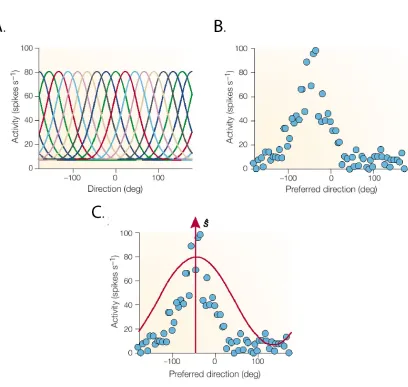
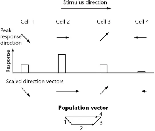
(23) 16 and Abbott, 2001; Rieke et al., 1997). This remains true regardless of whether stimulus reconstruction is actually performed by the animal in the same manner as it is evaluated experimentally. Several different classes of reconstruction methods have been developed, including population vector coding, Bayesian inference, and spike train decoding. Each technique has advantages in certain situations and challenges with respect to its implementation in a real neural system.. 1.4.1 Population Vector Coding Tuning curves are a way of describing the preferential activity that certain cells exhibit for a specific range of a continuous parameter. These curves are specific to each cell and are measured empirically by presenting a wide range of stimuli while monitoring the responses. Cells that demonstrate tuning curves have been identified in many sensory and motor systems, and typically groups of cells cover an entire stimulus range with their preferred response ranges (Fig. 1.2A) (Pouget et al., 2000; Rieke et al., 1997). Population vector coding uses tuning curves as the basis for calculating the “direction” of a stimulus or output (Dayan and Abbott, 2001; Foldiak, 2002; Oram et al., 1998). The preferential response of a given cell (its tuning curve) is mathematically represented as a direction vector with a magnitude equal to the difference between the given cell’s activity (over a specific time period) and the mean activity of that neuron in all conditions (Fig. 1.2B). By sampling from a large group of cells and summating the resulting vectors, a population vector can be created which represents the collective direction of the population’s activity (Fig. 1.3). Extensions of this method include multi-dimensional scaling of the individual cell vectors (Oram et al., 1998), which allows other applications that are not purely directional (e.g., face cells (Young and Yamane, 1992)), and methods for optimizing the coefficients used to estimate the vector direction (Dayan and Abbott, 2001). This method has been used with great success for predicting arm movements in monkeys.

(24) 17 (Schwartz and Moran, 2000), deciphering place cell function in the hippocampus (Zhang et al., 1998), and other similar applications.. Figure 1.2 Tuning Curves. A. Several different tuning curves each with a preferred response direction that collectively cover a range of values. B. An example of the data that is used to calculate a given cell's tuning curve. C. Preferential direction and cosine waveform superimposed upon example data. Figure adapted from Pouget et al., 2000.. However, there are problems with this method (Foldiak, 2002). First, tuning curves may not have the properties necessary for accurate decoding. Neurons in real systems do not always have tuning curves that are evenly distributed across the entire range of values, which can lead to bias in the resulting population vector. Also, tuning curves may not have a cosine function shape, which would also bias the vector. Second, variability in the responses of individual neurons are.

(25) 18 completely ignored. While it is assumed that the neurons will retain the shape of their tuning curve under all conditions, this may not be the case. Third, the method does not provide a mechanism to assess statistical confidence. Finally, the method is not easy to implement in neural systems. While this is not a requirement for decoding techniques, it does not argue in favor of this technique over others that have greater biological relevance.. Figure 1.3 Example calculation of a population vector for a horizontal stimulus from the responses of four neurons. Figure adapted from Foldiak, 2002.. 1.4.2 Bayesian Inference As the limitations discussed above indicate, population vector methods are neither a universal nor optimal way to decode stimuli. To overcome some of the problems associated with this technique, methods have been developed to eliminate tuning curves and instead evaluate probability distributions that associate stimuli with neuronal responses. These Bayesian methods are generally more applicable to different sensory/motor applications and allow one to quantify the quality of the reconstruction (Foldiak, 2002; Rieke et al., 1997). In addition, Bayesian.

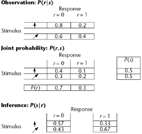
(26) 19 methods are easier to implement in realistic neural systems using feed-forward networks (Dayan and Abbott, 2001; Funahashi, 1998). At the core, Bayesian estimates involve determining the conditional probability that a response (r) will occur if a stimulus (s) is presented, P(r|s) (Fig1.4). The conditional probability of these two events occurring is related to the joint probabilities of each event occurring separately via Bayes’ rule: P(r|s) = P(r,s)/P(s).. EQ#1. However, in Bayesian decoding (working backwards from response to stimulus) one is interested in determining the reverse equation, termed the posterior distribution: P(s|r) = P(r|s)P(s)/P(r). EQ#2. P(s|r) = P(r,s)/P(r).. EQ#3.. or. To implement Bayesian decoding it is necessary to empirically determine the probability distributions for both the stimuli and responses. This can prove difficult because a large amount of data across a wide range of values is required. However, if the data is available, the values in the posterior distribution (EQ#2) are determined as follows: the histogram of responses across a range of stimuli provides P(r|s), P(s) is based on the characteristics of the known stimulus, and P(r) is determined with the relationship: P(r) = Σ(P(r|s)P(s)).. EQ#4. Once the posterior distribution, P(s|r), has been determined, additional manipulations must be performed to extract single values from this function. Essentially, extracting single values involves identifying the single value at the peak of the probability distribution; i.e., maximizing the function to find the direction of the highest probability density. However, the exact shape of a probability distribution is not known, and given any additional data it may change. In a sense this process underlies all Bayesian techniques: a prior distribution of data is.

(27) 20 refined as more data is presented, resulting in a distribution that more closely approximates the actual. One method, termed maximum a posteriori (MAP) estimation, accomplishes this task by minimizing a loss function that relates all possible peak values of the distribution to each hypothesized peak value and calculates a penalty. Minimizing this loss function is therefore equivalent to identifying the direction of highest probability density. A mathematical extension of this method is termed the maximum likelihood (ML) technique. ML arises logically from MAP in situations where a very large amount of data is present. In effect, these data allow one to base the entire estimate on observed data without any hypothesized prior distributions. It can be proven that in situations where the data set is sufficiently large, the ML method is optimal. Assessed theoretically, the ML method will approach an information-theory limit called the Cramer-Rao boundary, the theoretical limit for the accuracy of an unbiased estimator (Dayan and Abbott, 2001; Rieke et al., 1997).. Figure 1.4 An example of Bayesian decoding using two stimuli and two responses (0 or 1) from a single neuron. The probabilities of each stimulus, vertical or diagonal, occurring is 0.5. The conditional probability P(r|s) is measured separately for the two stimuli. Bayes' theorem gives the decoding for the two possible responses. Figure adapted from Foldiak, 2002..

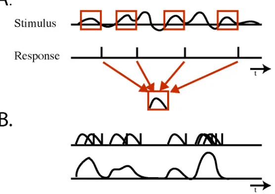
(28) 21 1.4.3 Spike-Train Decoding While vector and Bayesian methods are effective at decoding reasonably static stimuli, decoding stimuli that vary rapidly with time requires a different approach. Spike-train decoding is based on directly transforming spike trains from single cells or groups of cells into the stimuli that produced them. In conditions where a spike train closely and densely follows the evolution of a stimulus, a method using a linear combination of fixed kernels can be used; relating the occurrence of a spike to the preceding period of stimulus that generated it with time varying coefficients that are determined by the activity of individual cells (Bialek et al., 1991; Warland et al., 1997). Bialek and colleagues implemented this technique to decode the visual information present in the activity of the fly H1 neuron by using the following protocol (Bialek et al., 1991). A fly was presented with a grating pattern whose motion velocity varied randomly across its visual field. Simultaneously, the activity of the H1 neuron, which encodes the velocity and direction of a stimulus, was recorded extracellularly. After the experiment was complete, spiketriggered stimulus averages (STSAs) were created for each H1 cell (2, one in each eye, were recorded). These STSAs were calculated by averaging a fixed period (100ms) of the known stimulus that preceded each spike occurrence for each cell (Fig. 1.5A). Roughly, this process yields a kernel that relates a spike to the input stimulus that elicits it. By linearly summating the STSAs that correspond to each cell after convolving them with the recording of spike occurrences over the duration of the recording, they were able to reconstruct the major features of the original grating stimulus (Fig. 1.5B). One difficulty associated with this method is correctly determining the kernels. Bialek and colleagues addressed this issue by optimizing the STSAs in a recurrent process designed to minimize the reconstruction error over several iterations. At each step the quality of the reconstruction was tested with data that were not used in the original kernel construction. Overall, this method produced reconstructions that were very similar to the original time varying stimulus..

(29) 22. Figure 1.5 A. An example of the reverse correlation technique for extracting spike triggered stimulus averages (STSAs). A fixed period of time prior to each recorded spike is extracted from the stimulus recording and is averaged. B. Stimuli are reconstructed by combining the STSAs of each cell in accordance with the test spike pattern.. The work described in this dissertation will investigate applications of the spike-decoding method in the insect olfactory system. In that context this method will be used to provide the first high resolution reconstruction of an olfactory stimulus based solely on the activity of downstream neurons.. 1.5 Outline In this thesis I will investigate how information is encoded and decoded at various stages of the insect olfactory system. In particular, I will explore how this system responds to stimuli that are more naturalistic than those that have been used in previous work. I will test the applicability of our current theories in this different setting, determine if there are any conditions.

(30) 23 in which our current understanding does not hold, and remark upon behavioral experiments that could be implemented to determine the perceptual relevancy of this work. In the chapter 2 I will examine how the insect olfactory system responds to overlapping stimuli. Specifically, I will address certain paradoxes raised by our current model that inadequately explain situations where two odors are presented in a temporally overlapping fashion without being fully mixed. Several models, including dynamic resetting, have been proposed as solutions to this problem. The experiments that I will describe will sort through these competing theories and propose a new model for the processing of overlapping odors. In doing so I will investigate the role that prior conditions have on the ensemble processing of odors. Little is currently understood about how activated PN ensembles react when presented with a new odor. Applying analysis techniques partially developed in our laboratory, I will examine how PN ensemble representations adjust when odors are rapidly exchanged and investigate the downstream activity of the KCs to see if the activity predicted by the analysis is actually observed in the locust. Finally, this work will make predictions about unique overlapping odor conditions and the possibility that these states may lead to intermediate representations as a consequence of the coding principles used in the system - possibly causing the animal to experience perceptions that are unique from the individual components or their simple mixture. The work presented in this section has been submitted for publication as BM Broome, V Jayaraman, & G Laurent (2005). In chapter 3 I will investigate how the insect olfactory system reacts to rapidly varying odors, a situation that animals might encounter in nature. I will explore how PNs respond both individually and as groups, applying many of the same experimental techniques described above. I will explain new technologies developed to meet the specific needs of this project. Specifically, I will describe an electronic nose sensor that was adapted for use with electrophysiology to obtain high resolution records of odor stimuli. This sensor was essential for making new insights into the existence of unique classes of PNs and for decoding the odor stimulus from the resulting spike.

(31) 24 trains. I will describe the limited effects of history on PN activity in rapidly varying odor conditions and the unique odor specific responses that each cell can produce. Most significantly, I will propose that PN ensemble coding of odors fundamentally changes when odors are presented rapidly. Changes were observed in both the regions of odor space traversed and in the temporal response properties of the ensembles. Finally, detailed explanations will be given of the techniques that I used to reconstruct rapidly varying stimuli when single odors, overlapping odors, or complete mixtures of odors were present. Using these techniques I will explore how the quality of these reconstructions is dependent upon the number of cells used to create them. The work in this section is in preparation for publication as BM Broome, M Meister, & G Laurent (2005)..

(32) 25. Chapter 2. Encoding and Decoding of Overlapping Odor Sequences. 2.1 Introduction In nature, animals rarely encounter stimuli in isolation and must often extract meaningful information from complex streams of overlapping signals. With odors this undertaking is further complicated by the inherently chaotic and often unpredictable nature of these signals’ delivery (Koehl et al., 2001). Understanding how the brain treats such complex stimuli is further complicated by the observation that olfaction is a synthetic sense (Laing and Francis, 1989). That is, with the exception of specialized signals such as pheromones, allomones, or kairomones (Mustaparta, 1996; Suh et al., 2004; Vickers et al., 1998), odor segmentation appears to be limited in animals; similarly, humans can identify individual components in a mixture, but only if less than 3-4 odors are mixed together (Laing and Francis, 1989). How then, does the brain deal with multiple concurrent stimuli that are not correlated in time? Does it keep track of each one independently? Does it create a representation of the mixture when there is temporal overlap? Or does it behave yet differently? While the answers to these questions ultimately contain perceptual and behavioral components, we can begin to address them relatively easily using neurophysiological methods. In our case, the interest in such stimuli and their neural representations resides in the fact that they.

(33) 26 impose difficult constraints on the system; these constraints should in turn help us better understand the neural codes for odors. Our recent work on insects and fish olfactory systems shows that odors give rise to very different response profiles in two structures, separated by only one synapse (Friedrich and Laurent, 2001; Mazor and Laurent, 2005; Perez-Orive et al., 2002). In the antennal lobe odors are represented by distributed assemblies of promiscuous principal neurons, whose individual activities evolve deterministically over time in a PN- and odor-specific manner (Laurent and Naraghi, 1994; Laurent et al., 1996; Mazor and Laurent, 2005; Wehr and Laurent, 1996). In the mushroom body, the direct target of the antennal lobe, odors are represented by very small assemblies of highly specialized neurons called Kenyon cells, or KCs, that are silent at rest (Laurent and Naraghi, 1994; Perez-Orive et al., 2002). The mechanisms underlying this dramatic transformation of representations is beginning to be understood (Laurent, 1999; Perez-Orive et al., 2004; Perez-Orive et al., 2002): Kenyon cells accomplish a pattern matching between an activity (input) vector—a function of the state of the PN population at a given time— and a connectivity vector—the set of PNs that each KC connects to. With a large number of KCs (50,000 in a locust), a mushroom body can realize many different connection patterns and thus recognize many different PN activity patterns (R Jortner, SS Farivar, and G Laurent, in prep). Because each KC contacts about 50% of the PN population, differences between connectivity vectors can be maximized across the population (R Jortner, SS Farivar, and G Laurent, in prep), generating very different input specificities. For high specificity to arise, however, this pattern matching between input and connectivity vectors must occur over limited time windows: indeed, if KCs were allowed to summate their input over long periods of time, they would eventually reach spike threshold even when stimulated with suboptimal PN activity vectors. Our present understanding is that the relevant KC integration window corresponds to about one half of one oscillation cycle (about 20ms) (Perez-Orive et al., 2002; Wehr and Laurent, 1996). Thus, each KC is given one chance to fire during each oscillation cycle and repeated chances over successive cycles as long as PN.

(34) 27 output is synchronized: because PN activity vectors change from one oscillation cycle to the next (fast first, more slowly later) (Laurent et al., 1996; Mazor and Laurent, 2005; Stopfer and Laurent, 1999; Wehr and Laurent, 1996), each KC carries out a new pattern matching at each oscillation cycle. In other words, each KC action potential at a given time represents a specific instantaneous state of a large percentage of the PN population at that time. If this is true, the response of a KC should be very sensitive to the instantaneous variations of its input vector (instantaneous state of the PN population). Under conditions of overlapping stimuli, for example, one would predict that a KC that responds to odor A at time t would fail to fire if odor B were added to A a short time before t. Conversely, if a KC were found to respond at time t to a particular pattern of A-B stimulation, we predict that its response probability should drop as the relative timings of the A and B stimuli are changed. The stimulation paradigms we will explore here are therefore a means to explore the sensitivity of KCs to the instantaneous state of the PN population and to test our understanding of the decoding of PN activity by Kenyon cells.. 2.2 Results 2.2.1 PN Responses to Overlapping Odor Patterns PNs respond to odors (singular or mixtures) by producing both fast and slow temporally patterned responses. For each PN these responses are both highly reproducible and odor specific. We examine here the responses of PNs in conditions of staggered stimulations with two odors. As previously described (Stopfer et al. 2003; Mazor and Laurent, 2005) we performed extra-cellular simultaneous multi-single-unit recordings from groups of PNs (n = 87, avg. group size = 9, see Methods) while presenting 30 different stimulus conditions (10 to 15 trials each) composed of 6 pure odor conditions (citral x 2, geraniol x 2, no odor, paraffin oil) and 24 2-odor-pulse stimuli (Fig. 2.1A) in pseudo-random order. All stimuli were presented or mixed in a dry air carrier.

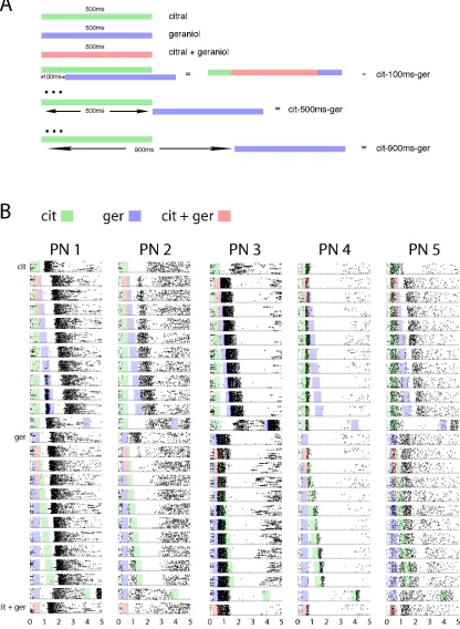
(35) 28. Figure 2.1, Stimulus Description and PN responses to Overlapping Stimuli A: Description of stimuli. Two odors, citral (cit) and geraniol (ger), were presented either alone or with a staggered onset times. In all cases each individual odor was presented for 500ms. The start times of the two odors were staggered relative to one another using the notation shown. The.

(36) 29 separation in odor start times ranged from 0ms (overlapping presentation, cit+ger) to 1s in steps of 100ms. An additional trial at 3.5s staggered onset was also included. B: Representative PNs displaying olfactory masking. Raster plots of 5 in vivo tetrode recordings from odor responsive locust PNs. Cells shown were not recorded simultaneously. Shaded areas correspond to pure and mixed odors indicated in legend and described in A. 15 consecutive trials per odor condition. Condition order was randomized within a given experiment.. stream (2 l/min). In all cases the responses of a given PN to an odor were highly reproducible across a block of 15 trials and across the course of an experiment (Fig. 2.1B). In locusts, PNs are the only antennal lobe neurons that produce sodium action potentials (Laurent and Davidowitz, 1994). Thus, all spikes reported here can be unambiguously attributed to PNs. PN responses to the two odors (citral, geraniol) or their mixture (citral + geraniol) contained excitatory and/or inhibitory epochs with odor- and PN- specific onset times and durations.. 2.2.2 Single PN Responses to Overlapping Odor Pulses Given the complex nature of PN responses to odors, we first examined whether the firing profiles of individual PNs to overlapping odor pulses could be predicted from the knowledge of their responses to each odor presented alone. Qualitative examples to each odor are shown for five PNs (Fig. 2.1B). While these five representative examples show different combinations of response types, the main interactions between overlapping pulses can be described as various forms of masking. When excitation by one of the two odors overlapped with inhibition caused by the other odor, excitation was generally reduced and sometimes totally suppressed. Consequently, one would predict that the detection of a component within a mixture from PN patterns alone should be compromised. We estimated the predictability of the interactions between firing rates (for each PN) by comparing observed and calculated firing rate profiles (Fig. 2.2A). These sums were calculated assuming that all cessation of firing, often caused by inhibition (Leitch and Laurent, 1996; MacLeod and Laurent, 1996), should be represented by the negative of the mean baseline-firing rate (see Methods). While this assumption may not be the best one, these.

(37) 30. Figure 2.2, Individual PN responses to overlap conditions are not simple summations of their responses to pure odor conditions. A: Three PNs responding to the various overlap conditions (gray) compared to the simple linear summation of their responses to pure odor conditions (red lines), with responses to the second odor shifted by the appropriate delay. Overlap conditions indicated by blue, green, and pale red bars in the background. Simple summation of pure condition responses matches PN1’s actual.

(38) 31 response fairly well for all overlap conditions. PN2 responds to most overlap conditions differently than might be expected from simple linear summation of its responses to the pure conditions. PN3 shows unexpectedly strong responses to geraniol when it is presented with a delay after citral. The response to geraniol in these cases is significantly stronger than both the linear summation and the response to either odor singly or the mixture (in the cit-900msec-ger condition, for example, the peak response to geraniol is twice as strong as when geraniol is presented by itself). B: The bar plot (test) shows the distribution of percentage deviations of estimated from measured firing rate (see Methods for an explanation of the computation) for all 87 recorded PNs (mean = 75%, SD = 22%). The green curve (control) shows the distribution of percent deviations calculated for all PNs (mean = 31%, SD = 17%) using only times of zero overlap (first 600ms following presentation of the first of two odors in conditions with 100ms or greater delays between pulses). Brown and green labels to the left of the arrows indicate difference ranges for PNs 1, 2, and 3 for overlap and non-overlap times respectively. C: Mean (over all PNs) percentage deviations for all overlap conditions plotted for each time bin (see Methods). Times of high deviation from summation-based estimates begin with the presentation of the second odor. Non-zero differences are seen even in the 3.5s delay condition, indicating that some PN responses at least are affected by history going back 3s.. comparisons were informative. They revealed, for example, that the response of a PN could match reasonably well (PN1, Fig. 2.2A), undershoot (PN2, Fig. 2.2A), or exceed (PN3, Fig. 2.2A) the simple sum of the component responses. Many of these more complex interactions could not be explained by an inadequate scoring of inhibition: the excess activity of PN3 (rows 812, Fig 2.2A) or the under-activity of PN2, (rows 3-8, Fig. 2.2A) for example, must be explained by other types of interactions, possibly involving receptor responses to mixtures, local circuit interactions within the antennal lobes, or likely, both. We then estimated the extent of these nonlinear interactions over all the recorded PNs. The distribution of differences between estimated (simple summation) and measured firing rate profiles during odor overlap conditions varied between 20 and 150%, with a mean of ~75% (Fig. 2.2B; also see Methods). PN1, PN2, and PN3 were -1.7, -0.9 and 1.55 SDs from the mean, respectively (brown labels next to arrows, Fig. 2.2B). As a control, we measured the distribution of differences measured between different trials of the same condition (green curve, Fig. 2.2B): for this we used the first 600ms of all odor overlap conditions with inter-pulse delays >100ms (i.e., cit-600ms-ger/ger-600ms-cit through cit3.5s-ger/ger-3.5s-cit). For 75 out of the 87 PNs, deviations were significantly higher during overlap conditions than in controls (Wilcoxon rank sum test, p<0.0001; see Methods and Fig..

(39) 32 2.2B). Large deviations between estimated (sums) and measured rates occurred at most times during and for some time after the presentation of the second odor (Fig. 2.2C) and could, in some PNs, be observed as late as 3s after the second pulse (yellow and orange pixels at ~4s in cit-3.5sger and ger-3.5s-cit rows in Fig. 2.2C).. 2.2.3 PN Population Responses to Overlapping Odor Pulses PNs were recorded from physically distributed areas across the AL in 10 animals. The number of simultaneously sampled PNs varied between 5 and 25. A recording site was chosen if at least some multi-unit activity could be recorded in response to each of the two odors and to a static mixture of the two odors at the beginning of each experiment. Only PNs that exceeded a set of equally applied inclusion criteria (see Methods) were selected (n = 87 PNs). In aggregate, this group represents more than 10% of the PN population in the antennal lobe. The spiking responses of each PN were analyzed in 50ms bins locked to the trial start time. 50ms bins corresponding to the mean duration of individual LFP oscillation cycles were chosen because they include the effective integration period of the PNs’ main target, the mushroom body Kenyon cells (PerezOrive et al., 2002). Recent experiments indicate that Kenyon cells each connect, on average, to 50 ±13% of the PN population and that their firing threshold corresponds to 100-200 coincident PN spikes (R Jortner, SS Farivar, and G Laurent, in prep). We also know that odor–evoked PN activity is composed of successive PN spike volleys (Laurent and Davidowitz, 1994), where each oscillation cycle contains the spikes of 80-240 PNs on average (Mazor and Laurent, 2005). We analyzed the representations of the odors and stimulus conditions as time series of PN population vectors (87 PNs, 50ms resolution, 30s trials, 15 trials per condition), as successfully applied previously to the encoding and decoding of odor concentrations (Stopfer et al., 2003)..

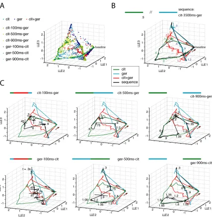
(40) 33 Figure 2.3 provides a pictorial representation of this population activity using locallylinear embedding (Roweis and Saul, 2000), a nonlinear dimensionality reduction technique useful for uncovering structure in high-dimensional space (Stopfer et al., 2003). These plots should be. Figure 2.3, PN ensemble responses track odor sequences. A: Time-slice points calculated from 87-PN responses to overlap sequences reduced to three dimensions using locally linear embedding. A subset of the original 5850 points embedded – only those for sequences shown in Fig. 2.3A,C – are shown here. Time slice points (50ms bins averaged over 3 trials) for the overlap sequences were taken beginning 0.5s before stimulus onset and ending 1 second after the end of the second stimulus. Correlations between 87-PN time slice vectors for these conditions are shown in Figures 2.4 and 2.5. B: Time-slice points in Fig. 2.3A.

(41) 34 were connected in sequence to visualize trajectories. Initially in a resting state (labeled “baseline”), the system responds with stimulus-specific trajectories. Shown as a control with trajectories for all pure conditions is the ensemble response to citral and geraniol presented with a gap of 3s between them – the trajectory for this sequence first follows the response to pure citral and then the response to pure geraniol. Five-trial averages for each condition; lines at vertices indicate S.D.; arrows indicate direction of motion. Time relative to odor onset indicated every 300ms. Color bars above plots in Fig. 2.3B,C indicate sequence presented. C: Trajectories in black show responses to 6 different overlap sequences with increasing delays in the presentation of the second odor (first row, citral followed by geraniol; second row, geraniol followed by citral). When switching from the first odor to the next, the system does not reset (return to baseline) and instead jumps to a later part of the second odor’s response. Ensemble responses to the second odor can be very different based on the duration of overlap (compare ger-100ms-cit sequence with ger-500ms- and ger-900ms-cit sequences).. read as qualitative indices of PN population state; quantitative analysis, carried out in the original high dimensional space, will be shown later. Figure 2.3A represents all the points (each point represents the state of the 87 PNs during one 50ms bin averaged over 3 trials) corresponding to six stimulus conditions in the space defined by the first three LLE dimensions. Baseline represents the state of the population prior to each stimulus (30s inter-trial interval). The points corresponding to successive time bins in the same trials were then joined together to generate stimulus specific trajectories (Fig. 2.3B&C). Figure 2.3B overlays the trajectories corresponding to four simple stimulus conditions: citral alone (green); geraniol alone (cyan); citral mixed with geraniol (red); citral followed 3.5s later by geraniol (black). We can see that the two odor pulses separated by 3.5s generated PN trajectories nearly identical to those generated by the same odors presented separately (i.e., with 30s interval or more). By contrast, the two odors presented simultaneously generated a hybrid response trajectory (red, Fig. 2.3B) that overlapped little with those of either odor alone, except well after termination of the stimulus pulse (at 0.5s). We will now examine several partial overlap conditions (Fig. 2.3C). In each case, the sequence trajectory is shown in black, overlaid on the three single trajectories shown in Fig 2.3B (green, cyan and red). In the top row citral was presented first; in the bottom row, the order was reversed. First we observed that the masking present in some single-PN responses is visible in these PN trajectories. In the ger-x ms-cit cases (bottom row, Fig. 2.3C), the trajectories process.

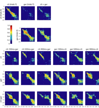
(42) 35 farther into the citral trajectory as the delay between pulses (x) increases from 100 to 900ms. This observation corresponds well with the increasing duration of some single-PN responses (PN1, Fig. 2.1B) under similarly varying conditions. Second, we noticed that the state of the PN. Figure 2.4 Correlation matrices for 87-PN time-slice vectors In the top two rows time slices from PN responses to the pure conditions are correlated with each other and with those of the odor mixture. The mixture response is different from both pure odor responses early and similar to the ger response late. In the lower three rows time slices from PN.

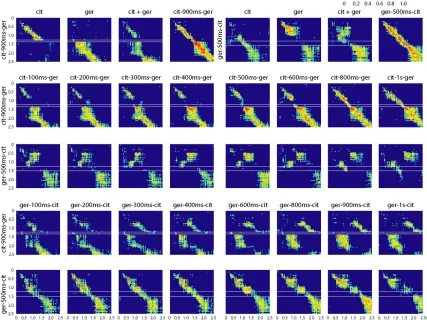
(43) 36 responses to these conditions are correlated with some of the conditions shown in Fig. 2.3B,C and Fig. 2.6. In correspondence with what is seen in the LLE plots (Fig. 2.3C), responses for the overlap conditions are first strongly correlated to the first odor presented and then switch, with a lag, to being correlated to the second or the mixture. Each pixel, Cr,c, represents the correlation of one 3-trial-averaged 87-PN time slice vector, r, with another, c, from either the same condition (but different 3-trial-averaged set) or a different condition, as indicated. Thus, a pixel Ct1,t2 represents the correlation of the time slice of trajectory A at time t1 to the time slice of trajectory B at time t2. All correlations shown are significant (p<0.001).. Figure 2.5 Correlation matrices for 87-PN time-slice vectors Correlations between time slices for different overlap responses. White rectangles highlight regions (times) where overlap responses show decreased or zero correlation with time slices from the pure conditions and with the mixture. These times and conditions match those revealed by MDA as being distant from both pure conditions and the mixture and for which unique KC responses were found. Note that the across-condition correlation levels at these times are not always zero; in some cases (see especially the last row for ger-500ms-cit) they are merely lower than at other times. Whether or not they are significant for the KCs (and ultimately for the animal) depends on the KCs’ sensitivities.. populations during an overlap condition depends on past history. For example, the cit-100ms-ger and ger-100ms-cit conditions produced 400ms of identical stimulus conditions (Fig 2.3C, left.

(44) 37 panels), yet the corresponding PN trajectories differed from each other and from that generated by the mixture (red, Fig. 2.3C). Third, for inter-pulse intervals of up to one second, the response of the PNs to the second pulse did not, even for an instant, pass through the baseline state. The trajectory corresponding to a sequence started as that for the first odor before moving towards the second. The sequence trajectory rejoined the second odor in segments corresponding to late phases of the second odor trajectory as if the second odor had been presented alone. This result suggests that, at least for epochs corresponding to the slow return to baseline after odor offset, the same PN population states can be reached through different paths or past histories. The cit500ms-ger trajectories (top row, middle graph, Fig. 2.3C) provide another illustration of this general observation, as the black and blue trajectories rejoin at t ≈ 0.9s. These results were not visible from inspection of single-PN activity profiles. This population vector analysis proved useful as a potential predictor of Kenyon cell responses. If our present understanding of PN activity decoding by Kenyon cells is correct (Mazor and Laurent, 2005; Perez-Orive et al., 2002; Stopfer et al., 2003), the orbits traced by the PN populations should define a variety of KC response conditions. For example, if the PN trajectories corresponding to an odor sequence move far away from the trajectories corresponding to either odor alone or to their mixture, we predict that some Kenyon cells should respond only to such sequence conditions and at particular times correspond to the structure of these trajectories. This hypothesis will be tested below. To identify these conditions, however, we needed to quantify the qualitative impression generated by the LLE projections in Fig. 2.3. Thus, we examined the PN population in the original 87-D space (using the same time bins and durations), one trial at a time, using multiple-discriminant-analysis (Fig. 2.6), a technique similar to multivariate analysis of variance (Duda et al., 2000). Our goal was to classify all the trajectories corresponding to overlapping stimuli on the basis of their similarity to single stimulus trajectories (citral alone, geraniol alone, citral + geraniol). This classification was done piecewise (time bin.

(45) 38 by time bin), against sixteen templates taken from the single-stimulus conditions (baseline + 3 odors x 5 time bins; Fig 2.6A, see Methods). 87-PN vectors from these sixteen.

No results found