warwick.ac.uk/lib-publications
Original citation:Hart, Sergiu, Kremer, Ilan and Perry, Motty. (2016) Evidence games : truth and commitment. American Economic Review.
Permanent WRAP URL:
http://wrap.warwick.ac.uk/82095
Copyright and reuse:
The Warwick Research Archive Portal (WRAP) makes this work by researchers of the University of Warwick available open access under the following conditions. Copyright © and all moral rights to the version of the paper presented here belong to the individual author(s) and/or other copyright owners. To the extent reasonable and practicable the material made available in WRAP has been checked for eligibility before being made available.
Copies of full items can be used for personal research or study, educational, or not-for-profit purposes without prior permission or charge. Provided that the authors, title and full
bibliographic details are credited, a hyperlink and/or URL is given for the original metadata page and the content is not changed in any way.
A note on versions:
The version presented here may differ from the published version or, version of record, if you wish to cite this item you are advised to consult the publisher’s version. Please see the ‘permanent WRAP URL’ above for details on accessing the published version and note that access may require a subscription.
Evidence Games: Truth and Commitment
1
Sergiu Hart
2Ilan Kremer
3Motty Perry
4September 13, 2016
1Previous versions: February 2014; May 2015 (Center for Rationality DP-684);
March 2016. The authors thank Maya Bar-Hillel, Elchanan Ben-Porath, Dan Bernhardt, Peter DeMarzo, Kobi Glazer, Ehud Guttel, Johannes H¨orner, Vijay Kr-ishna, Rosemarie Nagel, Michael Ostrovsky, David P´erez-Castrillo, Uriel Procac-cia, Phil Reny, Tom´as Rodr´ıguez-Barraquer, Ariel Rubinstein, Amnon Schreiber, Andy Skrzypacz, Rani Spiegler, Francesco Squintani, Yoram Weiss, and David Wettstein, for useful comments and discussions. We also thank the anonymous referees and the editor for their very careful reading and helpful comments and suggestions.
2Department of Economics, Institute of Mathematics, and Federmann
Cen-ter for the Study of Rationality, The Hebrew University of Jerusalem. Re-search partially supported by an Advanced Investigator Grant of the Eu-ropean Research Council (ERC). E-mail: [email protected] Web site: http://www.ma.huji.ac.il/hart
3Department of Economics, Business School, and Federmann Center for the
Study of Rationality, The Hebrew University of Jerusalem; Department of Eco-nomics, University of Warwick. Research partially supported by a grant of the European Research Council (ERC). E-mail: [email protected]
4Federmann Center for the Study of Rationality, The
Abstract
1
Introduction
1Ask someone if they deserve a pay raise. The invariable reply (with very few and, therefore, notable exceptions) is, “Of course.” Ask defendants in court whether they are guilty and deserve a harsh punishment, and the again invariable reply is, “Of course not.”
So how can reliable information be obtained? How can those who de-serve a reward, or a punishment, be distinguished from those who do not? Moreover, how does one determine the right reward or punishment when ev-eryone, regardless of information and type, prefers higher rewards and lower punishments?
These are clearly fundamental questions, pertinent to many important setups. The original focus in the literature was on equilibrium and equilib-rium prices. This approach was initiated by Akerlof (1970), and followed by the large body of work on voluntary disclosure, starting with Grossman and Hart (1980), Grossman (1981), Milgrom (1981), and Dye (1985). A related environment was considered by Green and Laffont (1986), but from a general mechanism-design viewpoint, where one can commit in advance to a policy. As is well known, commitment is a powerful device. The present pa-per nevertheless identifies a natural and important class of setups—which includes voluntary disclosure as well as various other models of interest— that we call “evidence games,” in which the possibility to commit does not
matter, namely, the equilibrium and the optimal mechanism coincide. This issue of whether commitment can help was initially addressed by Glazer and Rubinstein (2004, 2006) (see also Sher 2011).
Anevidence game is a standard communication game between an “agent” who is informed and sends a message (that does not affect the payoffs) and a “principal” who chooses the action (call it the “reward”). The two dis-tinguishing features of evidence games are, first, that the agent’s private information (the “type”) consists of certain pieces of verifiable evidence, and the agent can reveal in his message all this evidence (the “whole truth”),
1The reader is encouraged to consult the online Appendix C for additional results,
or only some part of it (a “partial truth”).2 The second feature is that the
agent’s preference is the same regardless of his type—he always prefers the reward to be as high as possible3—whereas the principal’s utility, which does
depend on the type, is single-peaked—he prefers the reward to be as close as possible to the “right reward.”
An essential feature of evidence games is the possibility of revealing the whole truth; the slight inherent advantage of the whole truth is used to select equilibria, which we calltruth-leaning equilibria. Specifically, these ob-tain from limits of perturbed games with infinitesimal increases in the agent’s utility when telling the whole truth, and in his probability of doing so. Truth-leaning thus amounts to the following two conditions: (i) when the reward for revealing a partial truth is the same as the reward for revealing the whole truth, the agent prefers to reveal the whole truth; and (ii) there is a small positive probability that the whole truth is revealed. These simple conditions are most natural, and they (and variants thereof) have been repeatedly used in the literature. The truth is after all a focal point, and there must be good reasons for not telling it. As Mark Twain wrote, “When in doubt, tell the truth,” and “If you tell the truth you don’t have to remember anything.” Truth-leaning turns out to be consistent with the various refinement condi-tions offered in the literature, and equivalent to many of them (such as the equilibria used in the voluntary disclosure literature).
To see the effect of commitment we consider the two distinct ways in which the interaction between the two players may be carried out. One way is for the principal to decide on the reward only after receiving the agent’s message; the other way is for the principal to commit to a reward policy, which is made known before the agent sends his message (i.e., the principal is the Stackelberg leader, which can only help him; this is the mechanism-design setup). Our equivalence result can be stated as follows:
In evidence games the truth-leaning equilibria without commit-ment yield the same (ex-post) payoffs as the optimal mechanisms with commitment.
2Try to recall the number of job applicants who included rejection letters in their files. 3This differs from signaling and screening setups, where costs depend on type, and
Simple examples that illustrate the result and the intuition behind it are provided in Section 1.1.
A number of comments are in order. First, the result implies in particular that among all Nash equilibria, the truth-leaning equilibria are optimal, i.e., most preferred by the principal.
Second, the “truth structure” of evidence games (which consists of the partial truth relation and truth-leaning) guarantees that commitment can-not yield any advantage. Whereas in the above-mentioned work of Glazer and Rubinstein (2004, 2006) and Sher (2011), the commitment outcome is obtained in some equilibrium of the game, but in general not in its other equilibria—and there is no good reason for the former to be picked out over the latter—in evidence games all truth-leaning equilibria yield the commit-ment outcome.
And third, the fact that commitment is not needed in order to guarantee optimality is a striking feature of evidence games; as we will show, the truth structure is indispensable to this result.
We stated above that evidence games constitute a very naturally oc-curring environment, which includes a wide range of applications and well-studied setups of much interest. We discuss here only two such applications. The first one deals with voluntary disclosure in financial markets. Public firms enjoy a great deal of flexibility when disclosing information. While disclosing false information is a criminal act, withholding information is al-lowed in some cases, and is practically impossible to detect in other cases. This has led to a growing literature in financial economics and accounting (see for example Dye 1985 and Shin 2003, 2006) on voluntary disclosure and its impact on asset pricing. The equilibria considered there turn out to be (outcome-equivalent to) truth-leaning equilibria, and so our result implies that the market’s equilibrium behavior is in fact optimal: it yields the opti-mal separation between “good” and “bad” firms (i.e., even with mechanisms and commitments—such as managers’ contracts—it is not worthwhile to sep-arate more).
precedents—which include inter alia rules of evidence. All this affects what evidence the parties (the “agents”) provide in court. An essential objective of the judicial criminal system is to induce the optimal amount of separa-tion between the guilty and the innocent and to get as close as possible to the right judgement (“fit the punishment to the crime”). Our result says that the power of these commitments does not, however, go beyond selecting among all equilibria the truth-leaning equilibria—which are most natural in this setup. A case in point is the legal doctrine known as “the right to remain silent.” In the United States, this right is enshrined in the Fifth Amendment to the Constitution, and is interpreted to include the provision that adverse inferences cannot be drawn, by the judge or the jury, from the refusal of a defendant to provide information. While the right to remain silent is now recognized in many of the world’s legal systems, its above interpretation re-garding adverse inference has been questioned and is not universal. The present paper sheds some light on this debate. First, because equilibria in general, and truth-leaning equilibria in particular, entail Bayesian inferences, the equivalence result implies that the same inferences apply to the optimal mechanisms; therefore, adverse inferences should be allowed, and surely not committedly disallowed. Second, truth-leaning may well replace commit-ment: rather than committing to rules such as the right to remain silent and its offshoots, one may instead strengthen and reinforce the (perceived) advantages of truth-telling. In England, for instance, an additional provi-sion (in the Criminal Justice and Public Order Act of 1994) states that “it may harm your defence if you do not mention when questioned something which you later rely on in court,” which may be viewed, on the one hand, as allowing adverse inference, and, on the other, as making the revelation of only partial truth possibly disadvantageous—which is the same as giving an advantage to revealing the whole truth (i.e., truth-leaning).
com-mitment; moreover, we show that the conditions of evidence games—most importantly, the truth structure—areindispensable conditions beyond which this equivalence no longer holds. In a nutshell, the paper identifies the nat-ural structure of evidence with its associated truth-leaning as the setup that guarantees that commitment cannot yield any advantage.
1.1
Examples
We provide two simple examples that illustrate the equivalence result and explain some of the intuition behind it.
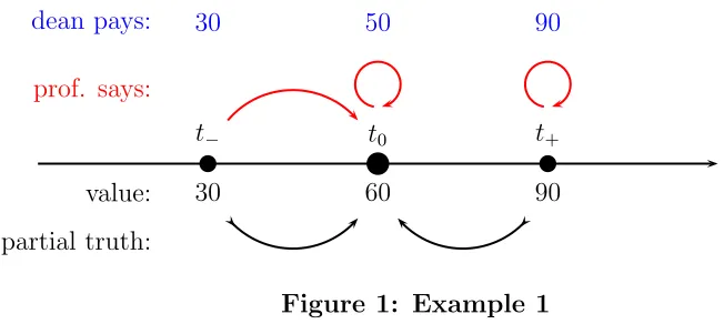
Example 1 A professor negotiates his salary with the dean. The dean would like to set the salary as close as possible to the professor’s “value,” while the professor would naturally like his salary to be as high as possible. The dean asks the professor if he can provide some evidence of his value (such as whether a recent paper was accepted or rejected, outside offers, and so on). Assume that with probability 50% the professor has no such evidence, in which case his (expected) value is 60, and with probability 50% he does have some evidence. In the latter case it is equally likely that the evidence is positive or negative, which translates to a value of 90 and 30,respectively. Thus there are three professor types: the “no-evidence” type t0, with
prob-ability 50% and value 60, the “positive-evidence” type t+, with probability
25% and value 90, and the “negative-evidence” type t−, with probability 25% and value 30. The professor can provide only evidence that he has, but he may choose which evidence to provide (thus, for example, t− can either reveal his evidence, or act as if he had no evidence, i.e., as if he were t0); see
the bottom arrows in Figure 1.
Consider first the game setup (without commitment): the professor de-cides whether to reveal his evidence, if he has any, and then the dean chooses the salary. It is easy to verify (see Appendix C.1) that there is a unique sequential equilibrium, where t+ reveals his positive evidence and is given a
30 60 90
t− t0 t+
value:
partial truth:
prof. says:
[image:9.595.110.436.126.272.2]dean pays: 30 50 90
Figure 1: Example 1
i.e., the expected value of the two types that provide no evidence: t0 andt−.
See the top arrows in Figure 1.
Next, consider the mechanism setup (with commitment): the dean com-mits to a salary policy (namely, three salaries, denoted by x+, x−, and x0,
for those who provide, respectively, positive evidence, negative evidence, and no evidence), and then the professor decides what evidence to reveal. One possibility is of course the above equilibrium: x+ = 90 and x− = x0 = 50.
Can the dean do better by committing? Can he provide incentives to the negative-evidence type t− to reveal his information? In order to separate and give different salaries to t− and t0 , the salary x− for those who provide negative evidence must be higher than the salaryx0 for those who provide no
evidence (i.e., x−> x0).Indeed, otherwise (i.e., whenx− < x0) the
negative-evidence type t− will pretend he is t0 and has no evidence and we are back
to the no-separation case. Since the value 30 of t− is lower than the value 60 of t0, setting a higher salary for t− than fort0 cannot be optimal (indeed,
decreasing x− and/or increasing x0 is always better for the dean, as it sets
the salary of at least one type closer to its value). The conclusion is that an optimal mechanism cannot separate t− from t0, and so the unique optimal
policy is identical to the equilibrium outcome, which is obtained without commitment.4 ¤
4
By contrast, t+ is separated from t0, because the value of t+ is higher. In general,
The following slight variant of Example 1 shows the use of truth-leaning; the requirement of being a sequential equilibrium no longer suffices here.
Example 2 Replace the positive-evidence type of Example 1 by two types: a (new) positive-evidence type t+ with value 102 and probability 20%, and
a “medium-evidence” type t± with value 42 and probability 5%. The type t± has two pieces of evidence: one is the same positive evidence that t+
has, and the other is the same negative evidence that t− has (for example, an acceptance decision on one paper, and a rejection decision on another). Thus,t± may pretend to be any one of the four typest±, t+, t−,ort0.In the
sequential equilibrium that is similar to that of Example 1, types t+ and t± both provide positive evidence and get the salary x+ = 90, and types t0 and
t− provide no evidence and get the salary x0 = 50 (the salaries are equal to
the corresponding expected values). It is not difficult to see that this is also the optimal mechanism outcome.
Now, however, the so-called “uninformative equilibrium” (also known as “babbling equilibrium”) where the professor, regardless of his type, never provides any evidence, and the dean ignores any evidence that might be provided and sets the salary to the average value of 60—which is worse for the dean, as it yields no separation between the types—is also a sequen-tial equilibrium. This equilibrium is supported by the dean’s belief that it is much more probable that the out-of-equilibrium positive evidence is pro-vided by t± rather than by t+; such a belief, while possible in a sequential
equilibrium, appears hard to justify. The uninformative equilibrium is not, however, a truth-leaning equilibrium, as truth-leaning implies that the out-of-equilibrium message t+ is used infinitesimally by type t+ (for which it is
the whole truth), and so the reward there must be set to 102, the value of t+. ¤
Now, the simplicity of the above examples may be misleading, as in gen-eral the equilibria can be quite complex and involve no easy unravelings and thresholds (e.g., Examples 7 and 10 in Appendix B, where the agent’s
strategy must be mixed). Finally, for a simple illustration of how commit-ment may yield outcomes that are strictly better than anything that can be achieved without it, see Example 3 in Appendix B.1: it is a slight variant of the above examples but with the professor’s utility depending on type (and so it does not belong to the class of evidence games).
1.2
Related Literature
There is an extensive and insightful literature addressing the interaction be-tween a principal who takes a decision but is uninformed and an agent who is informed and communicates information, either explicitly (through mes-sages) or implicitly (through actions). Separation between different types of the agent may indeed be obtained when the types have different utilities or costs (as in signaling, screening, and cheap-talk setups).
When different types have different possible actions—such as different sets of messages—separation may be obtained even when the agent’s utility and cost are the same regardless of his information. Grossman and Hart (1980), Grossman (1981), and Milgrom (1981), who initiated the “voluntary disclosure” literature, showed that unraveling obtains as a result of it being commonly known that the agent is fully informed.
truth-leaning turns out to be a natural way to unify all these criteria.
In the mechanism-design framework where the principal commits to a reward policy before the agent’s message is sent, Green and Laffont (1986) were the first to consider the setup where types differ in the sets of possible messages that they can send. They show that a necessary and sufficient con-dition for the revelation principle to hold for any payoff functions is that the message structure be transitive—which is satisfied by the voluntary disclo-sure models, as well as by our more general evidence games. Ben-Porath and Lipman (2012), Kartik and Tercieux (2012), and Koessler and Perez-Richet (2014) characterize the social choice functions that can be implemented when agents can also supply hard proofs about their types. Our social objective can be viewed as maximizing the fit between types and rewards.
The issue of comparing equilibria and mechanisms originated in Glazer and Rubinstein (2004, 2006). They analyze the optimal mechanism-design problem for general type-dependent message structures, with the principal taking a binary decision of “accepting” or “rejecting”; the agent, regardless of his type, prefers acceptance to rejection. They show that the resulting optimal mechanism can be supported as an equilibrium outcome; Sher (2011) extended the result to the case in which the decision is no longer binary, provided that the principal’s payoff is concave. By comparison, our paper shows that, in the framework of an agent with type-independent utility, the addition of the “truth structure” of evidence games—by which we mean the partial truth relation together with the truth-leaning behavior—yields the stronger result of the equivalence between the resulting equilibria and optimal mechanisms.5 Finally, an example where commitment does not help
in a disclosure game is included in Bhattacharya and Mukherjee (2013).
2
The Model
There are two players, an agent “A” and a principal “P.” The agent’s infor-mation is his type t, which belongs to a finite set T,and is chosen according
5Our companion paper Hart, Kremer, and Perry (2016) that deals with randomized
to a given probability distributionp= (pt)t∈T in ∆(T),the set of probability distributions on T, with pt > 0 for all t ∈ T. The agent knows the realized type t inT, whereas the principal knows only the distributionp but not the realized type.
The general structure of the interaction is that the agent sends amessage, which consists of a type sinT,and the principal chooses anaction, which is a real number xin R. The message is costless: it does not affect the payoffs of the agent and the principal. An interpretation to keep in mind is that the type corresponds to the (verifiable) evidence that the agent possesses, and the message corresponds to the evidence that he reveals.
A fundamental assumption of the model (which distinguishes it from the signaling and cheap-talk setups) is that all the types of the agent have the
same preference, which is strictly increasing in x (and does not, as already stated, depend on the message sent). Without loss of generality (only the ordinal preference matters here) we assume that the agent’s payoff is xitself, and refer to x as the reward (to the agent).
As for the principal, his utility does depend on the typet,but, again, not on the message s; thus, letht(x) be the principal’s utility for typet ∈T and reward x ∈ R (and any message s ∈ T). For every probability distribution q = (qt)t∈T ∈∆(T) on the set of types T—think of qas a “belief” on types— the expected utility of the principal is given by hq(x) := Pt∈T qtht(x) for eachx∈R.The functions ht are assumed to bedifferentiable and to satisfy:
(SP) Single-Peakedness. For every q∈∆(T) the principal’s expected utility hq(x) is a single-peaked function of the reward x.
A differentiable real function f : R→R is single-peaked if there exists a point v ∈ R such that f′(v) = 0; f′(x) > 0 for x < v; and f′(x) < 0 for x > v. Thus f has a global maximum at v, is strictly increasing for x ≤ v, and strictly decreasing for x≥v.
the examples in the Introduction). Similarly, v(q) is the ideal reward, or the value, when the types are distributed according to q.
Some instances where the single-peakedness condition (SP) holds are:
• Basic example: Quadratic loss. Each ht is the quadratic distance from the ideal point: ht(x) = −(x−v(t))2. In this case, common in much of the literature, the peak of hq is easily seen to be the expectation with respect to
q of the peaks v(t); i.e., v(q) = Pt∈Tqtv(t).
• Strict concavity. Each ht is a strictly concave function that attains its (unique) maximum at a finite point (which implies that the same holds for any weighted averages of such functions). For instance, ht is the negative of some distance (not necessarily quadratic) from the ideal point v(t).
•Monotonic transformations. Apply a strictly increasing transformation to the variable x, which preserves (SP) (but not concavity).
•Treat types differently, such as making differenthtmore or less sensitive to the distance from the corresponding ideal point v(t); e.g.,ht(x) =−ct|x−
v(t)|γt (with c
t > 0 and γt > 1, so as to get strict concavity). Also, the penalties for underestimating vs. overestimating the desired ideal point may be different: take the function ht to be asymmetric around v(t).
We assume here that there are no further randomizations on the rewardx. In case lotteries onxare allowed, the above single-peakedness condition is no longer sufficient and needs to be adapted; we analyze this in the companion paper Hart, Kremer, and Perry (2016). When all the functionshtare concave, the restriction to pure rewards is easily seen to be without loss of generality: replace every lottery by its expectation.
We conclude with a useful property of single-peakedness.
In-betweenness property of the peaks. Letx0 := mint∈T v(t) and x1 :=
maxt∈T v(t); because all the functions ht(x) are strictly increasing forx≤x0
and strictly decreasing for x ≥ x1, the peaks v(q) for all q ∈ ∆(T) satisfy
x0 ≤ v(q) ≤ x1. More generally, if q is a weighted average of q1, q2, ..., qn in ∆(T), i.e., q =Pni=1λiqi with Pni=1λi = 1 andλi >0 for all i, then
min
(indeed, all the functions hqi(x), and hence also hq(x) = Pni=1λihqi(x), are strictly increasing for x ≤ miniv(qi) and strictly decreasing for x ≥ maxiv(qi)). In particular, if T is partitioned into disjoint nonempty sub-sets T1, T2, ..., Tn then min1≤i≤nv(Ti) ≤ v(T) ≤ max1≤i≤nv(Ti), where v(T) stands forv(p) andv(Ti) forv(p|Ti) (withpthe prior andp|Tithe conditional of p given Ti). The rewards may thus be restricted to the compact interval
X = [x0, x1] that contains all the peaks: any reward x outside X is strictly
dominated for the principal (by x0 whenx < x0 and byx1 when x > x1).
2.1
Evidence and Truth
The agent’s message may be only partially truthful and he need not reveal everything that he knows; however, he cannot transmit false evidence, as any evidence disclosed is assumed to be verifiable. Thus, the agent must “tell the truth and nothing but the truth,” but not necessarily “the whole truth.”
Let E be the set of (verifiable) pieces of evidence. A type t is identified with a subset Et of E, namely, the set of pieces of evidence that the agent of type t can provide (e.g., prove in court). The possible messages of t are then either to provide all the evidence that he has (Et , “the whole truth”), or to pretend to be another type s with less evidence (i.e., Es ⊆ Et) and provide only the pieces of evidence in Es (a “partial truth”).6 Thus the set of possible messages of the agent when the type is t, which we denote by L(t), is identified with the set of types that have less evidence (in the weak sense) than t, i.e., L(t) := {s ∈ T : Es ⊆ Et}. This is immediately seen to entail two conditions:
(L1) t∈L(t) for every type t∈T;
(L2) if s∈L(t) and r ∈L(s) thenr ∈L(t).
(L1) says that revealing the whole truth is always possible: t can always say t. (L2) is a transitivity condition: if s has less evidence than t and r has
6The restriction that messages correspond to undetectable deviations (i.e., possible
less evidence than s, then r has less evidence than t; that is, if t can say s and s can say r thent can also say r. These conditions are standard; see for instance Green and Laffont (1986), Bull and Watson (2007), and Appendix C.3. From now on we abstract away from any specific setup and just assume (L1) and (L2).
Remark. A type t thus has two characteristics: his value to the principal (expressed by the function ht and its peak v(t)) and the evidence that he can provide (expressed by L(t)). We emphasize that no relation is assumed between value and evidence; in particular, having more evidence need not be associated with having a higher (or lower) value.
2.2
Game and Equilibria
We start by considering thegame Γ where the principal moves after the agent (and cannot commit to a policy). First, the typet ∈T is chosen according to the probability measure p∈∆(T), and revealed to the agent but not to the principal. The agent then sends to the principal one of the possible messages s in L(t). Finally, after receiving the message s, the principal decides on a reward x∈R.
A strategy σ of the agent associates with every type t∈ T a probability distribution σ(·|t) ∈ ∆(T) with support included in L(t); i.e., σ(s|t), which is the probability that type t sends the message s, satisfies σ(s|t) > 0 only if s ∈ L(t). A strategy ρ of the principal assigns to every message s ∈ T a reward ρ(s)∈R.
(A) for every type t ∈ T and message s ∈ T: if σ(s|t) > 0 then ρ(s) = maxs′∈L(t)ρ(s′);
(P) for every message s∈ T: if ¯σ(s) >0 then hq(s)(ρ(s)) = maxx∈Rhq(s)(x)
(and so ρ(s) =v(q(s)) by the single-peakedness condition).
The outcome of a Nash equilibrium (σ, ρ) is the resulting vector of rewards π = (πt)t∈T ∈RT, where, for every type t∈T,
πt:= max
s∈L(t)ρ(s); (2)
when the type istthe payoffs areπtfor the agent andht(πt) for the principal.
2.2.1 Truth-Leaning Equilibria
As discussed in the Introduction, evidence games may have many equilibria; we are interested in those in which truth enjoys a certain prominence. This is expressed in two ways. First, if it is optimal for the agent to reveal the whole truth, then he prefers to do so (this holds for instance when the agent has a “lexicographic” preference: he always prefers a higher reward, but if the reward is the same whether he tells the whole truth or not, he prefers to tell the whole truth). Second, there is an infinitesimal probability that the whole truth is revealed (which happens, for example, when the agent is not strategic and instead always reveals his information; or, when there are “trembles,” such as a slip of the tongue, or of the pen, or a document that is attached by mistake, or the surfacing of an unexpected piece of evidence). To formalize this we use a standard limit-of-small-perturbations approach. Specifically, givenεt >0 andεt|t>0 for everyt∈T (denote such a collection of ε-s by ε), let Γε denote the following perturbation of the game Γ. First, the agent’s payoff increases by εt when the type is t and the message s is equal to the type t; i.e., his payoff is equal to the reward x when s 6=t, and to x+εt when s = t. Second, the agent’s strategy σ is required to satisfy
a limit point of Nash equilibria of Γε
as all the ε-s converge to 0; i.e., if there are sequences εn
t →n→∞ 0, εnt|t→n→∞ 0, and (σn, ρn)→n→∞ (σ, ρ) such that (σn, ρn) is a Nash equilibrium of Γεn
for every n.
In terms of the original game, truth-leaning turns out to be essentially equivalent to imposing the following two conditions on a Nash equilibrium (σ, ρ) of Γ:
(A0) for every type t∈T: if ρ(t) = maxs∈L(t)ρ(s) then σ(t|t) = 1;
(P0) for every message s ∈ T: if ¯σ(s) = 0 then hs(ρ(s)) = maxx∈Rhs(x) (and so ρ(s) =v(s) by the single-peakedness condition).
Condition (A0) says that when the message t is optimal for type t, it is chosen by t for sure (i.e., if the whole truth is optimal then it is strictly preferred to any other optimal message). Condition (P0) says that, for every messages ∈T that is not used in equilibrium (i.e., ¯σ(s) = 0), the principal’s belief if he were to receive messages would be that it came from typesitself (since there is an infinitesimal probability that type s revealed the whole truth); thus the posterior belief q(s) at s puts probability one on s, and so the principal’s optimal response is the peak v(s) of hq(s) ≡ hs. For a rough intuition, (A0) obtains from the positive bonus in payoff, and (P0) from the positive probability of revealing the type (if s is not used then it is not a best reply for sby (A0), and so for no other type by transitivity (L2), which implies that in Γε only s itself uses s with positive probability). We state this formally in Proposition 1, which allows us to conveniently use only (A0) and (P0) in the remainder of the paper.
Proposition 1 (i) Truth-leaning equilibria exist. (ii) For every truth-leaning equilibrium (σ, ρ) there is an equilibrium (σ′, ρ) that satisfies (A0) and (P0)
and has the same outcome π as (σ, ρ).
The proof is relegated to Appendix A. Truth-leaning may thus be viewed as an equilibrium selection criterion (a “refinement”); alternatively, as part of the setup (the actual game being Γε
2.3
Mechanisms and Optimal Mechanisms
We come now to the second setup, where the principal moves first and com-mits to a reward scheme, i.e., to a functionρ: T →R that assigns to every message s ∈ T a reward ρ(s). The reward scheme ρ is made known to the agent, who then sends his message s, and the resulting reward is ρ(s) (the principal’s commitment to the reward schemeρmeans that he cannot change the reward after receiving the message s).
This is a standard mechanism-design framework. The reward scheme ρ is themechanism. Givenρ,the agent chooses his message so as to maximize his reward; thus, the reward when the type is t equals πt := maxs∈L(t)ρ(s).
A reward scheme ρ is an optimal mechanism if it maximizes the principal’s expected payoff
H(π) =X t∈T
ptht(πt) (3)
among all mechanisms.
The assumptions that we have made on the truth structure, i.e., (L1) and (L2), are easily seen to imply that the “Revelation Principle” applies: any mechanism can be implemented by a “direct” mechanism in which it is optimal for each type to be “truthful” and reveal his type; see Green and Laffont (1986), or Appendix C.5. The incentive compatibility constraints are
(IC) πt ≥πs for every t, s∈T with s∈L(t)
(indeed, s ∈L(t) impliesL(t)⊇L(s) by the transitivity condition (L2), and so πt = maxr∈L(t)ρ(r) ≥ maxr∈L(s)ρ(r) = πs). Thus an optimal mechanism outcome is a vector π= (πt)t∈T ∈RT that maximizesH(π) subject to (IC).
3
The Equivalence Theorem
Our main result is
The intuition is roughly as follows. Consider a truth-leaning equilibrium where a type t pretends to be another type s. Then, first, type s reveals his type s (had s something better, t would have it as well); and second, the value of s must be higher than the value of t (no one will want to pretend to be worth less than they really are).7 Thus t and s are not separated in
this equilibrium, and we claim that they cannot be separated in an optimal mechanism either: the only way for the principal to separate them would be to give a higher reward to t than to s (otherwise t would pretend to be s), which is not optimal since the value of t is lower than the value of s (decreasing the reward of t or increasing the reward of s would bring the rewards closer to the values). The conclusion is that optimal mechanisms can never separate more than truth-leaning equilibria do (the converse is immediate since whatever can be done without commitment can clearly also be done with commitment).
Remarks. (a) Outcomes. The Equivalence Theorem is stated in terms of outcomes—which uniquely determine the (ex-post) payoffs of both the agent and the principal for every typet. While there may be multiple truth-leaning equilibria, this can happen only when both players are indifferent, and then the payoffs are the same (see Appendix B.9).
(b) Tightness of the result. All the assumptions except differentiability are indispensable to the Equivalence Theorem: dropping any single condition yields examples where the result does not hold (see Appendix B). As for dif-ferentiability, it is only a convenient technical assumption, as the equivalence result holds also without it (see Appendix C.10).
(c) Constrained Pareto efficiency. In the basic quadratic-loss case, where, as we have seen, v(q) equals the expectation of the values v(t) with re-spect to q, condition (P) implies that the ex-ante expectation of the re-wards, i.e., E[πt] = Pt∈T ptπt, equals the ex-ante expectation of the values
E[v(t)] = Pt∈T ptv(t) = v(T) (because E[πt|s] = v(q(s)) = E[v(t)|s] for every message s that is used; take expectation over s). Therefore all Nash equilibria yield to the agent the same ex-ante expected payoff E[πt] = v(T)
7However reasonable these conditions may seem, they neednot hold for equilibria that
(they differ ex post, however, in the way this amount is split among the types). Since, by the Equivalence Theorem, the truth-leaning equilibria max-imize the principal’s ex-ante expected payoff, it follows that the truth-leaning equilibria are constrained Pareto efficient (i.e., ex-ante Pareto efficient among all equilibria).
4
Proof of the Equivalence Theorem
The proof proceeds as follows. We start with some useful and interesting properties of truth-leaning (Section 4.1), and then prove that the outcome of any truth-leaning equilibrium outcome is an optimal mechanism outcome, which is moreover unique (Section 4.2). Together with the existence of truth-leaning equilibria (Proposition 1(i) in Section 2.2.1) this yields the result.
4.1
Preliminaries
Proposition 3 Let (σ, ρ) be an equilibrium that satisfies (A0) and (P0), let
π be its outcome, and let S :={t∈T : ¯σ(t)>0} be the set of messages used in equilibrium. Then
t∈S ⇔ σ(t|t) = 1 ⇔ v(t)≥πt=ρ(t) ; and (4)
t /∈S ⇔ σ(t|t) = 0 ⇔ πt > v(t) =ρ(t). (5)
Thus, the reward ρ(t) assigned to message t never exceeds the peak v(t) of typet.Moreover, each typetthat reveals the whole truth gets an outcome that is at most his value (i.e., πt ≤v(t)), whereas each typet that does not reveal the whole truth gets an outcome that exceeds his value (i.e.,πt > v(t)). This may sound strange at first. The explanation is that the lower-value types are the ones that have the incentive to pretend to be a higher-value type, and so each message t that is used is sent by t as well as by “pretenders” of lower value. In equilibrium, this effect is taken into account by the principal by rewarding messages at their true value or less.
t ∈ L(t′)); (A0) then yields σ(t|t) = 1. This proves the first equivalence in (4) and in (5).
If t /∈ S then πt > ρ(t) (since t is not a best reply for t) and ρ(t) = v(t) by (P0), and hence πt > v(t) =ρ(t).
Ift ∈S then πt =ρ(t) (since t is a best reply for t); put α :=πt=ρ(t). Let t′ 6= t be such that σ(t|t′) > 0; then π
t′ = ρ(t) ≡ α (since t is optimal for t′); moreover, t′ ∈/ S (since σ(t|t′) > 0 implies σ(t′|t′) < 1), and so, as we have just seen above, v(t′) < π
t′ ≡ α. If we also had v(t) < α, then the in-betweenness property (1) would yield v(q(t)) < α (because the support of q(t), the posterior after message t, consists of t together with all t′ 6= t with σ(t|t′) >0). But this contradicts v(q(t)) = ρ(t)≡ α by the principal’s equilibrium condition (P). Therefore v(t)≥α ≡πt =ρ(t).
Thus we have shown thatt /∈S andt∈Simply contradictory statements (πt > v(t) and πt ≤ v(t), respectively), which yields the second equivalence in (4) and in (5).
Corollary 4 Let (σ, ρ) be an equilibrium that satisfies (A0) and (P0). If
σ(s|t)>0 for s=6 t then v(s)> v(t).
Proof. σ(s|t) > 0 implies s ∈ S and t /∈ S, and thus v(s) ≥ ρ(s) by (4), πt> v(t) by (5), and ρ(s) =πt because s is a best reply for t.
Thus, no type will ever pretend to be a lower-valued type (this does not, however, hold for equilibria that arenot truth-leaning, e.g., the uninformative equilibrium in Example 2 in the Introduction).
4.2
From Equilibrium to Mechanism
This section proves that any truth-leaning equilibrium outcome is an optimal mechanism outcome and, moreover, that the latter is unique. We first deal with a special case where there is no separation, and then show how a truth-leaning equilibrium yields a decomposition into instances of this special case.
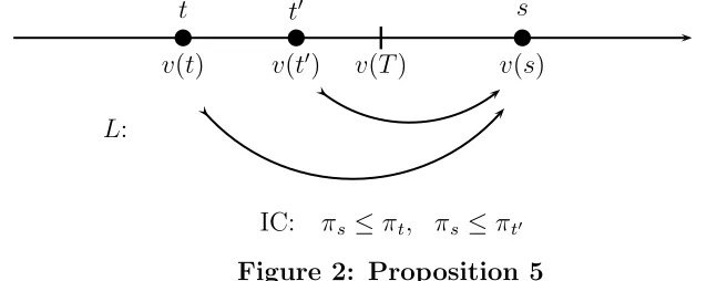
Proposition 5 Assume that there is a type s ∈ T such that s ∈ L(t) for every t. If v(t) < v(T) for every t 6= s then the outcome π∗ with π∗
for all t ∈T is the unique optimal mechanism outcome; i.e., X
t∈T
ptht(πt)≤
X
t∈T
ptht(π∗t) (6)
for every incentive-compatible π, with equality if and only if πt =π∗t =v(T)
for all t ∈T.
Thus every type can pretend to be s, and so s has the least amount of evidence (e.g., no evidence at all). The conditionv(t)< v(T) for every t6=s implies that v(T)≤v(s) by in-betweenness (1), and so v(t)< v(s) for every t 6=s; see Figure 2. To get some intuition, consider the simplest case of only two types, say, T = {s, t}. Because the (IC) constraint πt ≥ πs goes in the opposite direction of the peaks’ inequality v(t) < v(s), it follows that the maximum of H(π) =pshs(πs) +ptht(πt) subject to πt ≥πs is attained only when πt and πs are equal. Indeed, if πt > πs then we must have πt > v(t) or πs < v(s), and so decreasing πt or increasing πs brings it closer to the corresponding peak, and hence increases the value of H. Thus πt =πs =x for some x, and then the maximum is attained when x equals the peak of hp(x) = pshs(x) +ptht(x), i.e., when x=v(T).
Proof. First, v(t) < v(T) for all t 6= s implies by in-betweenness (1) that v(R)≥v(T) for every setR ⊆T that contains s.Next, letπmaximizeH(π) subject to the (IC) constraints; we will show that π must equal π∗ (which satisfies all (IC) constraints, as equalities).
Putα:= mintπtandR:={r∈T :πr =α}. Because one may change the common value of πr for allr∈R to anyα′ close enough toαso that all (IC)
v(t) v(t′) v(T) v(s)
t t′ s
L:
[image:23.595.121.449.582.709.2]IC: πs ≤πt, πs ≤πt′
inequalities continue to hold (specifically, α′ ≤β whereβ := min
t /∈Rπt > α), the optimality ofπimplies thatαmust maximizePt∈Rptht(x) =p(R)hR(x), and soα=v(R).ButRcontainss(because the (IC) constraints includeπs≤
πt for all t 6= s), and so α =v(R)≥ v(T). Therefore H(π) =
P
tptht(πt)≤
P
tptht(α) =hT(α)≤hT(v(T)) =
P
tptht(π∗t) =H(π∗) (the first inequality because πs =α,and fort6=sthe functionht(x) decreases after its peakv(t) and πt ≥ α ≥ v(T) > v(t); the second inequality because hT(x) decreases after its peak v(T) and α ≥ v(T)). Moreover, all the above functions are strictly decreasing after their peaks, and so to get equalities throughout we must have πt=α=v(T) for all t, i.e., π=π∗.
Proposition 6 Letπ∗ be a truth-leaning equilibrium outcome; thenπ∗ is the
unique optimal mechanism outcome.
Proof. Let (σ, ρ) be an equilibrium that satisfies (A0) and (P0) and has outcome π∗ (by Proposition 1). Because π∗ satisfies (IC) by (L2), we need to show that H(π∗)> H(π) for everyπ 6=π∗ that satisfies (IC).
Let S :={s ∈ T : ¯σ(s) >0} be the set of messages that are used in the equilibrium (σ, ρ), and, for each s ∈S, letTs:={t ∈T : σ(s|t)>0} be the set of types that play s. For every t 6= s in Ts we then have s ∈ L(t) and
t /∈ S (because σ(s|t) < 1 implies σ(t|t) < 1), and so v(t) = ρ(t) < π∗ t =
π∗
s = ρ(s) = v(q(s)) (by (5) and (4) in Proposition 3, and the principal’s equilibrium condition (P)). We can therefore apply Proposition 5 to the set of types Ts with the distribution q(s) as prior, to get (6) for every π that satisfies (IC), with equality only if πt =π∗t for every t∈Ts.
For anyπ ∈RT,the principal’s payoff H(π) can be decomposed as
H(π) =X t∈T
ptht(πt) =
X
s∈S ¯
σ(s)X t∈Ts
qt(s)ht(πt). (7)
References
Akerlof, G. A. (1970), “The Market for ‘Lemons’: Quality Uncertainty and the Market Mechanism,” Quarterly Journal of Economics 84, 488–500.
Ben-Porath, E. and B. Lipman (2012), “Implementation with Partial Prov-ability,” Journal of Economic Theory 147, 1689–1724.
Bhattacharya, S. and A. Mukherjee (2013), “Strategic Information Revela-tion when Experts Compete to Influence, ”RAND Journal of Economics
44, 522–544.
Bull, J. and J. Watson (2007), “Hard Evidence and Mechanism Design,
Games and Economic Behavior 58, 75–93.
Crawford, V. and J. Sobel (1982), “Strategic Information Transmission,”
Econometrica 50, 1431–1451.
Dye, R. A. (1985), “Strategic Accounting Choice and the Effect of Alternative Financial Reporting Requirements,”Journal of Accounting Research 23, 544–574.
Glazer, J. and A. Rubinstein (2004), “On Optimal Rules of Persuasion,”
Econometrica 72, 1715–1736.
Glazer, J. and A. Rubinstein (2006), “A Study in the Pragmatics of Persua-sion: A Game Theoretical Approach,”Theoretical Economics 1, 395–410.
Goltsman M., J. H¨orner, G. Pavlov, and F. Squintani (2009), “Mediation, Arbitration and Negotiation,” Journal of Economic Theory 144, 1397– 1420.
Green, J. R. and J.-J. Laffont (1986), “Partially Verifiable Information and Mechanism Design,” The Review of Economic Studies 53, 447–456.
Grossman, S. J. (1981), “The Informational Role of Warranties and Private Disclosures about Product Quality,” Journal of Law and Economics 24, 461–483.
Grossman, S. J. and O. Hart (1980), “Disclosure Laws and Takeover Bids,”
Journal of Finance 35, 323–334.
Hart, S., I. Kremer, and M. Perry (2016), “Evidence Games with Randomized Rewards,” working paper.
Kartik N. and O. Tercieux (2012), “Implementation with Evidence,” Theo-retical Economics 7, 323–355.
Krishna, V. and J. Morgan (2007), “Cheap Talk,” in The New Palgrave Dictionary of Economics, 2nd Edition.
Koessler, F. and E. Perez-Richet (2014), “Evidence Based Mechanisms,” working paper.
Milgrom, P. R. (1981), “Good News and Bad News: Representation Theo-rems and Applications,” Bell Journal of Economics 12, 350–391.
Pae, S. (2005), “Selective Disclosures in the Presence of Uncertainty About Information Endowment,” Journal of Accounting and Economics 39, 383–409.
Sher, I. (2011), “Credibility and Determinism in a Game of Persuasion,”
Games and Economic Behavior 71, 409–419.
Shin, H. S. (2003), “Disclosures and Asset Return,” Econometrica 71, 105– 133.
A
Appendix: Proof of Proposition 1
We prove here Proposition 1 in Section 4.1: first, the existence of truth-leaning equilibria, and second, their payoff equivalence to equilibria that satisfy (A0) and (P0). The former is a standard fixed-point proof, while the latter turns out to be somewhat more delicate than the intuitive arguments in Section 4.1 may suggest; in particular, it uses the differentiability of the functions8 h
t.
Proof of Proposition 1. (i) Existence. First, a standard fixed-point argument shows that the game Γε
possesses a Nash equilibrium. Let Σε be the set of strategies of the agent in Γε
; then Σε
is a compact and convex subset of ∆(T)T. Every σ in Σε uniquely determines the principal’s best replyρ≡ρσ byρσ(s) =v(q(s)) for every s∈T (cf. (P); in Γε
every message is used: ¯σ(s) ≥ εsps > 0). The mapping from σ to ρσ is continuous: the posteriorq(s)∈∆(T) is a continuous function ofσ (because ¯σ(s) is bounded away from 0), and v(q) is a continuous function of q (by the Maximum Theorem together with the single-peakedness condition (SP), which gives the uniqueness of the maximizer). The set-valued function Φ that maps each σ ∈Σε
to the set of all σ′ ∈Σε
that are best replies to ρσ in Γε
is therefore upper hemicontinuous, and a fixed point of Φ, whose existence is guaranteed by the Kakutani fixed-point theorem, is precisely a Nash equilibrium of Γε
. Second, the strategy sets of the two players are compact (for the principal, see in-betweenness in Section 2), and so limit points of Nash equilibria of Γε
— i.e., truth-leaning equilibria of Γ—exist (it is immediate to verify that any limit point of Nash equilibria of Γε
is a Nash equilibrium of Γ, i.e., satisfies (A) and (P)).
(ii) (A0) and (P0). Let (σ, ρ) be a truth-leaning equilibrium, given by sequences εn
t →n 0+, εnt|t→0+, and (σn, ρn)→n(σ, ρ) such that (σn, ρn) is a Nash equilibrium in Γεn
for everyn (which is easily seen to imply that (σ, ρ) is a Nash equilibrium of Γ, i.e., that (A) and (P) hold).
Lett be such that σ(t|t)<1.Thenσ(s|t)>0 for somes 6=t inL(t),and soσn(s|t)>0 for all (large enough) n. In Γεn
we thus have: s is a best reply
8
for t, hence ρn(s) ≥ρn(t) +εn
t > ρn(t), hence t is not optimal for any r 6=t (because t∈L(r) implies s∈L(r) by transitivity (L2) ofL and s gives to r a strictly higher payoff thant in Γεn
), and thus σn(t|s) = 0.Taking the limit yields:
if σ(t|t)<1 then σ(t|s) = 0 for all s6=t; (8)
this says that if t does not choose t for sure, then no other type chooses t. Moreover, the posterior qn(t) after message t puts all the mass on t (since
σn(t|t) ≥ εn
t|t > 0 whereas σn(t|s) = 0 for all s 6=t), i.e., qn(t) = 1t, and so
ρn(t) =v(qn(t)) = v(t); in the limit:
if σ(t|t)<1 then ρ(t) =v(t). (9)
This in particular yields (P0), because ¯σ(t) = 0 implies σ(t|t) = 0<1. To get (A0) we may need to modify σ slightly, as follows. Let t ∈ T be such that t is a best reply for t (i.e., ρ(t) = maxs∈L(t)ρ(s)) but σ(t|t) < 1.
Then ρ(t) =v(t) by (9), and every messages6=t thatt uses, i.e.,σ(s|t)>0, gives the same reward as message t, and so v(q(s)) = ρ(s) = ρ(t) = v(t). Therefore we define σ′ to be identical to σ except that type t chooses only message t; i.e., σ′(t|t) = 1 and σ′(s|t) = 0 for every s6=t.
Let q′(s) be the new posterior after a message s 6=t that was used by t (i.e., σ(s|t) > 0; note that ¯σ′(s) ≥ p
s > 0 since σ′(s|s) = σ(s|s) = 1 by (8) applied to s). Let α:=v(q(s)) = v(t) (see above); using the differentiability of the functions hr we will show that the peak ofhq′(s) is also at9 α. Indeed, q(s) is a weighted average of q′(s) and 1
t, and so hq(s) is a weighted average
of hq′(s) and ht. The derivatives of hq(s) and ht both vanish atα, and so the derivative ofhq′(s) must also vanish there—thusv(q′(s)) =α =v(q(s) =v(t). It follows that (σ′, ρ) is a Nash equilibrium of Γ: the agent is indifferent between the messages t and s, and the principal maximizes his payoff also at the new posterior q′(s). Clearly (8) and (9), and hence (P0), continue to hold; moreover, the outcome remains the same. Proceeding this way for every t as needed will in the end yield also (A0).
9Example 12 in Appendix C.10 shows that this property neednot hold without
B
Appendix: Tightness of the Equivalence
Theorem
We will show here that our Equivalence Theorem is tight. First, we show that dropping any single assumption (except for differentiability, which is assumed for convenience; see Appendix C.10) allows examples where the equivalence between optimal mechanisms and truth-leaning equilibria does not hold (Sections B.1 to B.7). Second, we show that the conclusions cannot be strengthened; specifically, truth-leaning equilibria need be neither pure nor unique (Sections B.8 and B.9).
B.1
Agent’s Payoffs Depend on Type
We provide a slight variant of the examples in the Introduction (which can also be easily restated in the standard Crawford and Sobel 1982 cheap-talk setup) that shows that the equivalence result may fail when the agent’s types do not all have the same preference: commitment strictly helps here.
Example 3 There are only two types of professor, and they are equally likely: t0,with no evidence and value 60, andt−,with negative evidence and value 30. As above, the dean wants to set the salary as close as possible to the value, and t0 wants as high a salary as possible. However, t− now wants his salary to be as close as possible to 50 (for instance, getting too high a salary would entail duties that he does not like): his utility when he gets salary xis −(x−50).
Consider now the mechanism where the salary policy is to pay 30 when negative evidence is provided, and 75 when no evidence is provided. Since t−prefers 30 to 75, he will reveal his evidence, and so separation is obtained. The mechanism outcome is better for the dean than the equilibrium outcome (he makes an error of 15 for t0 only in the mechanism, and an error of 15
for both types in equilibrium). Note that the above mechanism requires the dean to commit to pay 75 when he gets no evidence; otherwise, after getting no evidence (which happens when the type is t0), he will want to
change his decision and pay 60 instead. In general, commitment is required when implementing reward schemes that are not ex-post optimal (our result implies that this does not happen in evidence games; the requirement that is not satisfied in Example 3 is that the agent’s utility be the same for all types). ¤
Remarks. (a) Two optimal mechanisms are as follows: the salaries are set to 30 for negative evidence and 70 for no evidence in the first, and to 40 and 60, respectively, in the second; in both mechanisms, t−, who is indifferent between revealing and concealing his evidence, reveals it.
(b) Taking the utility of t0 to be −(x−80)2, which does not affect the
example, sets it in the standard Crawford and Sobel (1982) cheap-talk setup. The fact that commitment may be advantageous in cheap-talk games is known; see Krishna and Morgan (2007) and Goltsman et al. (2009).
B.2
Without Reflexivity (L1)
We provide an example where the condition (L1) that t ∈L(t) for all t∈T is not satisfied—some type cannot tell the whole truth and reveal his type— and there is a truth-leaning Nash equilibrium whose payoffs are different from those of the optimal mechanism.
The unique optimal mechanism outcome isπ0 =v(0) = 0 andπ2 =π4 =
v({2,4}) = 3, i.e.,10 π = (π
0, π2, π4) = (0,3,3).
Truth-leaning entails no restrictions here: types 0 and 2 each have a single message (their type), and type 4 cannot send message 4. There are two Nash equilibria: (i) 4 sends message 2, ρ(0) = 0, ρ(2) = 3, with outcome π = (0,3,3) (which is the optimal mechanism outcome); (ii) 4 sends message 0, ρ(0) = 2, ρ(2) = 2,with π′ = (2,2,2). Note that H(π)> H(π′). ¤
B.3
Without Transitivity (L2)
We provide an example where (L2) is not satisfied—the “less evidence” rela-tion is not transitive—and there is a truth-leaning equilibrium outcome that is different from the optimal mechanism outcome.
Example 5 The type space is T = {0,2,4} with the uniform distribution: pt= 1/3 for eacht ∈T.The principal’s payoff functions areht(x) =−(x−t)2, and so v(t) = t for all t. The allowed messages are L(0) = {0,4}, L(2) =
{2}, and L(4) ={2,4}. This does not satisfy (L2): type 0 can send message 4 and type 4 can send message 2, but type 0 cannot send message 2.
The unique optimal mechanism is given by11 the reward scheme ρ =
(0,3,0), with outcome π = (0,3,3); indeed, if 2 and 4 are separated then it is best to set ρ(2) = v(2) = 2 and ρ(4) = v({0,4}) = 2, yielding the outcome π′ = (2,2,2); and if they are not separated then it is best to set ρ(2) = v({2,4}) = 3 and ρ(0) = ρ(4) = v(0) = 0, yielding the outcome π = (0,3,3); the latter is better: H(π) = −2/3>−8/3 =H(π′).
There is no equilibrium satisfying (A0) and (P0) with outcomeπ: type 0 must use 0 (by (A0), because ρ(0) =π0),types 2 and 4 must use 2 (because
π2 = π4 = 3), but then 4 is unused and so ρ(4) = v(4) = 4 (by (P0)),
contradicting (P).
10When writing vectors such as π the coordinates are ordered according to increasing
value; thus here we haveπ= (π0, π2, π4) (recall thatv(t) =t).
11While type 0 can send message 4, he cannot fully mimic type 4, because he cannot
Both π and π′ are truth-leaning equilibrium outcomes:12 take Γε with εt=εt|t=εfor allt; then πobtains from the limit of13 σε(·|0) = (ε,0,1−ε),
σε(·|4) = (0,1−ε, ε),and ρε = (0,3−ε/(2−ε),4ε); andπ′ obtains from the limit of σε(·|0) = (ε,0,1−ε), σε(·|4) = (0,0,1),and ρε = (0,2,4/(2−ε).
¤
B.4
Without (A0)
We provide an example of a sequential equilibrium that does not satisfy the (A0) condition of truth-leaning, and whose outcome differs from the unique optimal mechanism outcome.
Example 6 The type space is T = {0,2,4} with the uniform distribution: pt= 1/3 for eacht∈T.The principal’s payoff functions areht(x) = −(x−t)2 (and so v(t) = t) for each t ∈ T. Type 0 has less evidence than type 4, who has less evidence than type 2; i.e., L(0) = {0}, L(2) = {0,2,4}, and L(4) ={0,4}.
The unique optimal mechanism outcome isπ= (0,3,3),and in the unique equilibrium that satisfies (A0) and (P0) types 2 and 4 send message 4 (type 0 must send 0) and14 ρ = (0,0,3). There is however another (sequential)
equilibrium: type 2 sends message 4 and type 4 sends message 0, and ρ′ = (2,2,2),with outcomeπ′ = (2,2,2),which is not optimal (H(π′)< H(π)).At this equilibrium (P0) is satisfied (since ρ′(2) =v(2) for the unused message 2), but (A0) is not satisfied (since message 2 is optimal for type 2 but he sends 4). ¤
B.5
Without (P0)
Example 2 in the Introduction has an equilibrium (the uninformative equi-librium) that satisfies (A0) but does not satisfy (P0), and its outcome differs
12Once we go beyond our setup, the outcome equivalence given in Proposition 1 between
truth-leaning and (A0)+(P0) need no longer hold.
13σε(·|0) = (ε,0,1−ε) means that σε(s|0) =ε,0,1−εfors= 0,2,4, respectively (the order on types is again increasing in value); similarly forρε.
from the unique optimal mechanism outcome. However, that specific equilib-rium can be ruled out by requiring the belief of the principal after an unused message to be equal to the conditional probability over the set of types that can send that message. That is, if message t is unused then put q(t) = p|L−1(t), the conditional of the prior p over the set L−1(t) := {r ∈ T : t ∈
L(r)}of all typesrthat can send messaget,andρ(t) = v(q(t)) = v(p|L−1(t))
(instead of q(t) =1t and ρ(t) =v(t) in (P0)). The following example shows that replacing (P0) with this requirement is not enough to get equivalence.
Example 7 The type space is T = {0,3,10,11} with the uniform distri-bution: pt = 1/4 for each t. The principal’s payoff functions are ht(x) =
−(x−t)2 (and sov(t) =t) for eacht∈T.Types 10 and 11 both have less
ev-idence than type 0,and more evidence than type 3; i.e.,L(0) ={0,3,10,11}, L(3) ={3}, L(10) ={3,10},and L(11) ={3,11}.
The unique equilibrium that satisfies (A0) and (P0) is mixed: σ(·|0) = (0,0,3/7,4/7),all the other types t6= 0 reveal their type, and ρ= (0,3,7,7) (use for instanceL′ as in Appendix C.7 (b); note thatv(q(10)) =v(q(11)) = v({0,10,11}) = 7). The unique truth-leaning and optimal mechanism out-come is thus π = (7,3,7,7).
Consider now the uninformative equilibrium where every type sends mes-sage 3 and ρ = (0,6,5,5.5) (note that ρ(3) = v(T) = 6); its outcome π′ = (6,6,6,6) is different from π. This equilibrium satisfies (A0) (because type 3 sends message 3) but not (P0) (for types 10 and 11). However, it does satisfy the alternative condition above: ρ(0) = v(L−1(0)) = v(0) = 0,
ρ(10) = v(L−1(10)) =v({0,10}) = 5,and ρ(11) =v(L−1(11) =v({0,11}) =
5.5.¤
B.6
Without Payoff or Probability Boost
Example 8 The type space isT ={0,2,4,6}with the uniform distribution: pt= 1/4 for eacht∈T.The principal’s payoff functions areht(x) = −(x−t)2 (and so v(t) = t) for each t ∈ T. The mapping L is L(0) = {0,4}, L(2) =
{0,2,4,6}, L(4) ={4},and L(6) ={4,6} (e.g., type 4 has no evidence, type 0 has a piece of negative evidence, type 6 has a piece of positive evidence, and type 2 has both pieces of evidence; this is the same evidence structure as in Example 2 in the Introduction15).
The unique optimal mechanism outcome is π = (2,4,2,4), and in the unique equilibrium that satisfies (A0) and (P0) types 0 and 4 send message 4 and types 2 and 6 send message 6.
The uninformative equilibrium where every type uses message 4 and the outcome is π′ = (3,3,3,3) (with H(π′) = −5< −4 = H(π)) is the limit of Nash equilibria (σε, ρε) of Γε
with ε6 = 0 and all other εt and εt|t equal to
ε, as follows: σε(0|0) = σε(2|2) = σε(6|6) = ε, σε(6|2) = ε(6−5ε)/(2 +ε), and with the remaining probabilities every type uses 4; and ρε = (0,2,3− 4ε/(2−ε),3−4ε/(2−ε)).
If we instead takeε6|6 = 0 and all otherεt|tandεtto be equal toε,then the Nash equilibria of Γε
with σε(0|0) =σε(2|2) =ε, σε(4|0) =σε(4|2) = 1−ε,
σε(4|4) = σε(4|6) = 1, and ρε(0) = 0, ρε(2) = 2, ρε(4) = (6−ε)/(2 +ε) ≥
ρε(6) (message 6 is unused) again yield π′ in the limit.¤
B.7
Without (SP)
We provide an example where one of the functions ht is not single-peaked and all the Nash equilibria yield an outcome that is strictly worse for the principal than the optimal mechanism outcome.
Example 9 The type space is T = {1,2} with the uniform distribution, i.e., pt= 1/2 for t= 1,2.The principal’s payoff functionsh1 andh2 are both
strictly increasing for x < 0, strictly decreasing for x > 2, and piecewise linear16 in the interval [0,2] with values at x = 0,1,2 as follows: −3,0,−2
15The only reason that we do not work with Example 2 is that the numbers here are
smaller and easier to handle.
16The example is not affected if the two functions h
1, h2 are made differentiable (by
forh1,and 2,0,3 forh2.Thush1 has a single peak atv(1) = 1,whereash2 is
not single-peaked: its global maximum is atv(2) = 2,but it has another local maximum at x= 0.Type 2 has less evidence than type 1, i.e., L(1) ={1,2} and L(2) ={2}.
Consider first the optimal mechanism; the only (IC) constraint isπ1 ≥π2.
Fixingπ1 (in the interval [0,2]),the value ofπ2 should be as close as possible
to one of the two peaks of h2, and so either π2 = 0 or π2 = π1. In the
first case the maximum of H(π) is attained at π = (1,0), and in the second case, at π′ = (2,2) (because 2 is the peak ofh
p = (1/2)h1+ (1/2)h2). Since
H(π) = 1>1/2 =H(π′), the optimal mechanism outcome isπ = (1,0). Next, we will show that every Nash equilibrium (σ, ρ), whether truth-leaning or not, yields the worse outcome π′ = (2,2).Indeed, type 2 can only send message 2, and so the posterior q(2) after message 2 must put at least as much weight on type 2 as on type 1 (i.e., q2(2)≥1/2≥q1(2); recall that
the prior is p1 =p2 = 1/2). Therefore the principal’s best reply is always 2
(because hq(2)(0) <0, hq(2)(1) = 0, and hq(2)(2) > 0). Therefore type 1 will
never send the message 1 with positive probability (because thenq(1) = (1,0) and so ρ(1) = v(1) = 1 < 2). Thus both types only send message 2, and we get an equilibrium if and only if ρ(2) = 2 ≥ ρ(1) (and, in the unique truth-leaning equilibrium, (P0) implies ρ(1) = v(1) = 1), resulting in the outcome π′ = (2,2), which is not optimal: the optimal mechanism outcome is π = (1,0). ¤
Thus, the separation between the types—which is better for the principal— can be obtained here only with commitment.
B.8
Mixed Truth-Leaning Equilibria
We show here that we cannot restrict attention to pure equilibria: the agent’s strategy may well have to be mixed (Example 7 above is another such case).