Detecting Abrupt
Changes in Big Data
Kaylea Haynes, B.Sc.(Hons.), M.Res
Submitted for the degree of Doctor of
Philosophy at Lancaster University.
Kaylea Haynes, B.Sc.(Hons.), M.Res
Submitted for the degree of Doctor of Philosophy at Lancaster University. September 2016
Abstract
This thesis looks at developing methods for changepoint detection that can be used in the realm of Big Data. In particular we look at developing methods that can be scaled to the volume of data, now readily collected and stored, and are also versatile to the different varieties of data.
A well established approach to detect changes uses penalised optimisation where the choice of the penalty has a huge impact on the performance of the method. In the first part of this thesis we propose an algorithm, CROPS (Changepoints over a Range of PenaltieS), which finds the optimal solutions for a range of penalties instead of only specifying one penalty.
The second part of this thesis looks at the choice of cost function used in the optimisation. In particular we develop a computationally efficient method, which uses a nonparametric cost function, allowing for changes to be detected in a larger variety of data-sets. This nonparametric approach uses the empirical cumulative distribution of the data and thus does not require any assumptions to be made on distributional parameters.
The third part of this thesis looks at ways to parallelise detection methods in order to use multi-core computers and thus allowing for changes to be detected in much larger data-sets than they could be previously. We look at different ways to split the data across multiple cores and then merge the results to try to conserve as much of the accuracy that we had when we only used one core.
Acknowledgements
There are many people I need to thank whom this PhD would not have been possible without. First and foremost, I would like to thank my supervisors Professors Paul Fearnhead and Idris Eckley for all their help, support and patience throughout this PhD. I have learnt many lessons during this PhD from both Paul and Idris and for that I am very grateful. Thanks also to Dr Rebecca Killick for involving me in the changepoint R package and for all the insightful discussions over the past few years.
I am very grateful for the financial support provided by the EPSRC and DSTL. I would like to thank my industrial supervisor Ralph Mansson for his helpful conver-sations and for organising my trip to DSTL which gave me insight into working in industry. I also need to thank Vincent Brault for providing access to the Hi-C data used in Chapter 3.
I would like to thank all the staff at the STOR-i Centre for Doctoral Training for providing a stimulating and enjoyable research environment, as well providing many training opportunities. A special thanks to Professor Jonathan Tawn for his continuous words of support and guidance.
I would also like to thank all of the support staff at STOR-i and Lancaster Uni-versity. Especially to Cyrus Gaviri and Dave Sole who have provided me with lots of IT help and have helped sort out even my more awkward of computer problems.
My PhD experience would not have been what it is today without all the friends I have made along the way. A special thanks to the surviving students in my cohort: Christian, Ivar, Lawrence, Lisa and Monika, who have been on this journey with
me from the start. Their kindness, laughter and friendship has really helped make this experience enjoyable and helped me through the less fun parts. Thanks also to the changepoint reading group and the machine learning reading group for all of the interesting discussions but most importantly for all the coffee and cake!
On a more personal note I am very grateful to my parents and family for supporting me over the years though I’m sure they’ve been counting down the days to when I’m no longer living the student life.
Declaration
I declare that the work in this thesis has been done by myself and has not been sub-mitted elsewhere for the award of any other degree.
Chapter 3 has been accepted for publication as Haynes, K., Eckley, I.A., and Fearnhead, P. (2016). Computationally efficient changepoint detection for a range of penalties. Journal of Computational and Graphical Statistics.
Chapter 4 has been accepted for publication as Haynes, K., Fearnhead, P., and Eckley, I.A. (2016). A computationally efficient nonparametric approach for change-point detection. Statistics and Computing.
Kaylea Haynes
Acknowledgements II
List of Figures XII
List of Tables XIII
1 Introduction 1
2 Review of the Changepoint Literature 4
2.1 Applications . . . 4
2.2 Model . . . 8
2.3 Single Changepoint Detection . . . 8
2.4 Binary Segmentation and Variants . . . 10
2.4.1 Wild Binary Segmentation . . . 10
2.4.2 Circular Binary Segmentation . . . 11
2.5 Optimisation Problem . . . 12
2.5.1 Cost Functions . . . 13
2.5.2 Dynamic Programming . . . 15
2.5.3 Penalties . . . 19
2.5.4 Simultaneous Multiscale Changepoint Estimator . . . 21
2.6 Nonparametric Approaches . . . 21
2.7 Other Approaches . . . 24
2.7.1 Bayesian Methods . . . 24
CONTENTS VI
2.7.2 Hidden Markov Models . . . 25
2.7.3 Multivariate Methods . . . 26
2.7.4 Online/Sequential Changepoint detection . . . 28
2.8 High Performance Computing and Parallel Algorithms . . . 30
2.8.1 Architecture . . . 31
2.8.2 R Packages . . . 34
2.8.3 Parallel Algorithms . . . 34
3 Computationally Efficient Changepoint Detection for a Range of Penalties 37 3.1 Introduction . . . 37
3.2 Background . . . 41
3.2.1 Segment Costs . . . 41
3.2.2 Finding Optimal Segmentations . . . 42
3.2.3 Pruning Methods . . . 43
3.3 Algorithm for a Range of Penalty Values . . . 44
3.3.1 Link Between Optimisation Problems . . . 44
3.3.2 Theoretical Results . . . 46
3.3.3 The Changepoints for a Range of PenaltieS (CROPS) Algorithm 46 3.3.4 The Number of Changepoints that are Optimal for Some β . . 48
3.3.5 Computational Cost . . . 49
3.4 Simulation Study . . . 51
3.4.1 Change in Mean . . . 52
3.4.2 Change in Mean and Variance . . . 53
3.4.3 Evaluating the Choice of Penalty . . . 53
3.5 Application to Hi-C Data . . . 56
4 A Computationally Efficient Nonparametric Approach for
Change-point Detection 60
4.1 Introduction . . . 60
4.2 Nonparametric Changepoint Detection . . . 63
4.2.1 Model . . . 63
4.2.2 Nonparametric Maximum Likelihood . . . 64
4.2.3 Nonparametric Multiple Changepoint Detection . . . 64
4.2.4 NMCD Algorithm . . . 65
4.3 ED-PELT . . . 66
4.3.1 Discrete Approximation . . . 67
4.3.2 Use of PELT . . . 67
4.4 Results . . . 69
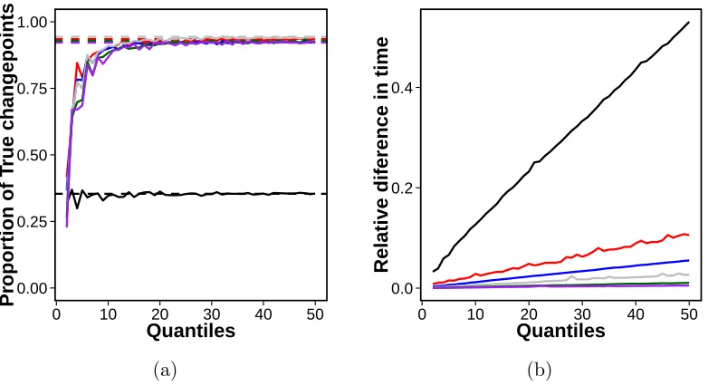
4.4.1 Performance of NMCD . . . 69
4.4.2 Size of Screening Window . . . 75
4.4.3 Choice of K in ED-PELT . . . 75
4.4.4 Comparison of NMCD and ED-PELT . . . 78
4.5 Activity Tracking . . . 79
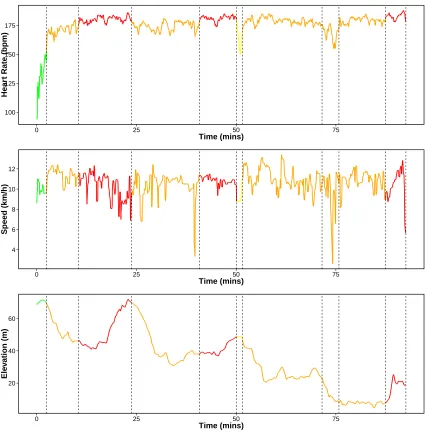
4.5.1 Changepoints in Heart-Rate Data . . . 79
4.5.2 Range of Penalties . . . 80
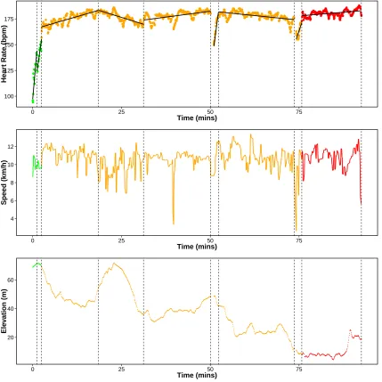
4.5.3 Piece-wise Linear Model . . . 84
4.6 Conclusion . . . 85
5 Parallel Changepoint Detection 88 5.1 Introduction . . . 88
5.1.1 Parallel Implementation . . . 90
5.2 Embarrassingly Parallel . . . 91
5.2.1 Binary Segmentation . . . 92
5.3 Dynamic Programming Algorithms . . . 95
CONTENTS VIII
5.3.2 Approach 1 . . . 96
5.3.3 Approach 2 . . . 97
5.3.4 Boundaries . . . 98
5.4 Simulations . . . 98
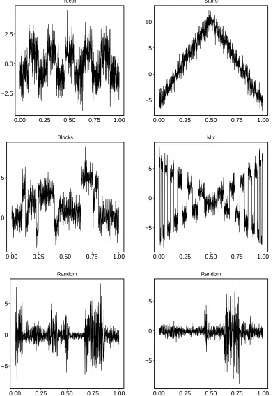
5.4.1 Signals . . . 98
5.4.2 Evaluation . . . 100
5.4.3 Detection Rate . . . 102
5.4.4 Speed . . . 108
5.5 Conclusion . . . 111
6 Conclusions and Future Directions 113 6.1 Future Directions . . . 115
6.1.1 Probabilistic Pruning . . . 115
6.1.2 Nonparametric Cost Functions . . . 117
6.1.3 Parallelising Multivariate Methods . . . 117
A Supplementary Material for Chapter 3 122 A.1 Pseudo-code for PELT . . . 122
A.2 Proof of Therem 3.1 . . . 123
A.3 Proof of Theorem 3.2 . . . 124
A.4 Further Simulations: Change in Mean . . . 125
A.5 Further Simulations: Change in mean and variance for normal model 125 A.6 Further Simulations: Change in Mean and Variance for the Mis-specified Model . . . 128
A.7 Further regions where we have discrepancies in the Hi-C example . . 129
B The CROPS Algorithm in the changepoint R Package 130 B.1 Usage . . . 130
C Supplementary Material for Chapter 4 133
C.1 Further Results - ED-PELT . . . 134
C.2 Further Results - Piece-wise linear . . . 137
D changepoint.np: An R Package for Nonparametric Changepoint De-tection 141 D.1 Package Structure . . . 142
D.1.1 Inputs . . . 142
D.1.2 Outputs . . . 143
D.2 Examples . . . 143
D.2.1 Simulated Data . . . 143
D.2.2 Heart-Rate Data . . . 144
E Further Simulation Results for Chapter 5 148 F R Code for the SM1 and SM2 methods proposed in Chapter 5 151 F.1 Package Structure . . . 151
F.1.1 Output . . . 152
F.1.2 Example . . . 152
List of Figures
1.1 Examples of changepoints . . . 2
2.1 Memory architectures . . . 31
2.2 Amdahl’s law . . . 33
3.1 Relationship between the constrained and penalised costs . . . 45
3.2 Cost for the segmentations against the number of changepoints . . . . 49
3.3 Simulations: CPU cost for the changes in mean . . . 52
3.4 Simulations: results for the true model . . . 55
3.5 Simulations: results for the mis-specified model . . . 55
3.6 Segmentations of chromosome 16 . . . 58
4.1 Exploration of the window size NI in NMCD+ . . . 76
4.2 Exploration of the number of quantiles K in ED-PELT . . . 77
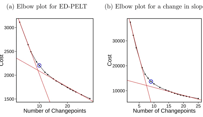
4.3 Cost vs number of changepoints for ED-PELT and change in slope . . 82
4.4 Segmentation of heart-rate using ED-PELT with 10 changes . . . 83
4.5 Segmentation of heart-rate using change in slope with 9 changes . . . 86
5.1 Computational time taken to run Binary Segmentation in parallel over multiple cores. . . 93
5.2 Example test signals . . . 101
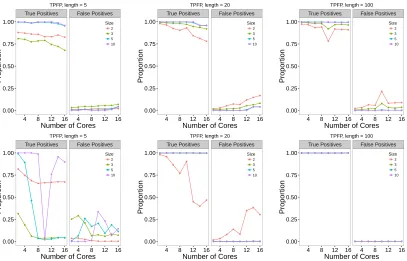
5.3 The true and false discovery rates for SM1 and SM2 on the teeth signal over a different number of cores. . . 103
5.4 The true and false discovery rates for SM1 and SM2 on the stairs signal
over a different number of cores. . . 104
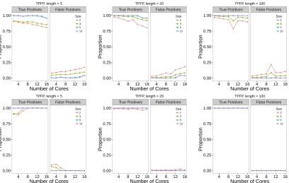
5.5 The true and false discovery rates for SM1 and SM2 on the blocks and teeth signal over a different number of cores. . . 105
5.6 The results of using SM1 on the teeth signal with different number of points around the boundary. . . 106
5.7 The results of using SM1 on the stairs signal with different number of points around the boundary. . . 107
5.8 The CPU time for SM1 and SM2 on the blocks signal of different lengths.109 5.9 The CPU time for SM1 and SM2 on the mix signal of different lengths, 110 5.10 The CPU time for SM1 and SM2 on the random signal of different lengths . . . 111
6.1 Changepoint vectors considered around the boundary in parallel mul-tivariate changepoint detection . . . 120
6.2 An illustration of the challenges of using a fixed boundary length. . . 121
A.1 Changes in mean CPU cost using pDPA and CROPS with FPOP . . 125
A.2 Changes in mean and variance using SN, CROPS with PELT and CROPS with PELT with the speed improvements . . . 126
A.3 Changes in mean and variance results when using the true model. . . 127
A.4 Results for the mis-specified model . . . 128
A.5 Further HIC segmentations . . . 129
C.1 Segmentations using ED-PELT with 13 changepoints . . . 134
C.2 Segmentations using ED-PELT with 12 changepoints. . . 135
C.3 Segmentations using ED-PELT with 9 changepoints. . . 136
C.4 Segmentations using change in slope with 12 changepoints . . . 137
C.5 Segmentations using change in slope with 10 changepoints . . . 138
LIST OF FIGURES XII
C.7 Segmentations using change in slope with 7 changepoints . . . 140
D.1 Plot of the changepoints using the plot method of the cpt class . . . . 145 D.2 Diagnostic plot for the heart-rate data-set when the CROPS penalty
is used. . . 146 D.3 Segmentation of the heart-rate data with 15 changepoints. . . 147
E.1 Further simulations for the true and false discovery rates for SM1 and SM2 on the teeth signal over a different number of cores. . . 149 E.2 Further simulations for the true and false discovery rates for SM1 and
4.1 True and false discovery rates and time comparisons for NCMD, NMCD+ and ED-PELT. . . 72 4.2 Over-segmentation and under-segmentation errors, and the number of
changepoints detected for NCMD, NMCD+ and ED-PELT. . . 74
Chapter 1
Introduction
High resolution data sensors are common-place in the devices which we use in our day to day lives. For example, mobile phones contain many sensors for measuring motion, orientation and environmental conditions (Android, 2016). Consequently we are now able to record and store more data than ever before. This has resulted in a resurgence of interest in a number of different inference areas, not least of which is changepoint analysis.
A changepoint (sometimes referred to as a breakpoint) is a point in a data-series,
for example a time-point or a position along a chromosome, where there has been a change in one or more of the statistical properties. Figure 1.1 shows example data-sets with (a) changes in mean, (b) changes in mean and variance and (c) changes in trend and variance. Knowledge of these changepoints is often invaluable for effective modelling and forecasting.
In this thesis we look at developing methods for changepoint detection that can be applied in the Big Data revolution. We will start by reviewing some of the vast literature of changepoint detection in Chapter 2. In particular we will focus our attention on methods for detecting multiple changes in a univariate, offline setting since this is the scenario of main interest throughout this thesis.
A popular approach for changepoint detection is to use penalised optimisation
0.0 2.5 5.0 7.5
0 250 500 750 1000 Index
Data
(a)
−10 0 10
0 250 500 750 1000 Index
Data
(b)
−30 −20 −10 0 10 20
0 250 500 750 1000 Index
Data
(c)
Figure 1.1: Examples of data-series with changes in one or more statistical property: (a) changes in mean, (b) changes in mean and variance and (c) changes in trend and variance.
which requires a choice of a penalty. Mis-specifying this penalty can have a detrimental effect in the performance of the changepoint detection method. In Chapter 3 we propose a new algorithm, CROPS (Changepoints over a Range Of PenaltieS), which finds the optimal solution over a range of penalties in a continuous range. We apply CROPS to detect genomic regions that interact through the folding and 3-D structure of a chromosome and show how we can choose the best segmentation once we have recovered the segmentations for all penalties in our given range. This chapter is published as the journal article Computationally Efficient Changepoint Detection for
a Range of Penalties in Journal of Computational and Graphical Statistics (Haynes
et al., 2017).
CHAPTER 1. INTRODUCTION 3
since we do not require any prior knowledge of the parameters. We apply this method to heart-rate data recorded during a period of physical activity and show that ED-PELT works better than using a cost function which assumes the data is normally distributed. This chapter is published as the journal article A computationally
effi-cient nonparametric approach for changepoint detection in Statistics and Computing
(Haynes et al., 2016).
There are two main approaches for solving the optimisation problem in change-point detection. The first is an approximate approach which involves recursively detecting single changepoints. The second uses dynamic programming which is an exact approach but can be computationally expensive and therefore do not scale well to large amounts of data. In Chapter 5 we show how we can utilise High Performance computing by parallelising the changepoint detection algorithms. We look at various ways to split the data across multiple cores and then merge the results without losing much accuracy.
Review of the Changepoint
Literature
In this Chapter we will review some of the changepoint literature, in particular we will look at methods for offline, multiple changepoint detection in univariate data. There are many researchers across a vast range of disciplines using and developing state of the art algorithms for changepoint detection. Changepoint detection was first used for quality control (Page, 1954) but ever since changepoints have been of interest across many different fields. Below are some examples of where the detection of changes can play an important, and sometimes even life changing, role. This is by no means an exhaustive list but it does highlight the variety of applications in which changepoint detection can be, and has been, used.
2.1
Applications
Genomics
In genomics changepoint detection has been used for DNA sequencing to identify pattens in the gene (Braun and M¨ueller, 1998; Braun et al., 2000). The DNA copy number of a region is the number of copies of genomic DNA. In humans, this copy
CHAPTER 2. LITERATURE REVIEW 5
number is two for all of the autosomes. To find the copy numbers on the genome, tech-niques such as comparative genomic hybridization (CGH) or array-based comparative genomic hybridization (array-CGH), for higher resolutions, are used. Changepoint de-tection is then used to find the regions where there is loss or amplification in tumour cells (Picard et al., 2004; Zhang and Siegmund, 2007). Variations in the copy number are common in cancer and other diseases (Olshen et al., 2004). Hocking et al. (2013b) review different methods for detecting changes in the chromosomal copy number. More recently Cleynen et al. (2013) apply changepoint detection to RNA-seq data which they claim will have improved accuracy over the use of CGH arrays. Cleynen et al. (2014) provide a recent comparison of segmentation methods on RNA-Seq data.
Environmental
In an environmental setting, changepoint detection can prove to be useful for logis-tical reasons, such as maintenance scheduling or managing resources. Wang et al. (2014) use changepoint detection to see if there has been changes in the monthly precipitation at various watersheds, across Southeast United States, due to climate change. In oceanography, Killick et al. (2013) and Nam et al. (2015) detect changes, and determine the uncertainty, in the autocovariance of wave heights, in the North Sea, to determine storm season changes. Reeves et al. (2007) provide a comparison of techniques used to detect changes in climate data, specifically they show examples of detecting changepoints in annual average temperature recorded in Alabama and Montana.
Finance and Economics
over-stated by not accounting for the breakpoints in the volatility. Finding the changes in volatility is required for risk management, forecasting and hedging (Fernandez, 2004). For example Aggarwal et al. (1999) use the changepoint detection method of Incl´an and Tiao (1994) to detect shifts in volatility in emerging markets, before examining the local and global events which happened at the time of the changes. Andreou and Ghysels (2009) discuss the implications of ignoring changepoints in financial data as well as review a number of different changepoint detection tests used to detect different changes in financial asset returns and volatility. Other authors consider multivariate series of daily stock indices (such as Lavielle and Teyssi`ere, 2006) or look at ways to detect changes as they happen in financial streams (Pepelyshev and Polunchenko, 2015).
Network Security
Cyber-attacks cost the UK economy billions of pounds every year. Computer net-works can be represented as a data stream (an unending sequence of data-points) in which deviations from the normal network behaviour could be a sign of an at-tack. Sequential changepoint detection methods, in particular anomaly detection, can be used as intrusion detection systems. Various methods have been proposed that include detection in univariate streams (see for example Kim et al., 2004; Tar-takovsky et al., 2013), Bayesian methods (Heard et al., 2010), nonparametric methods (L´evy-Leduc and Roueff, 2009) and detection in multivariate streams (Bodenham and Adams, 2013). Changepoint models have also been used to detect the attack of instant messaging worms (Yan et al., 2008).
Other
CHAPTER 2. LITERATURE REVIEW 7
the detection of changes in brain signals such as electroencephalograms (EEG) which can be used to understand the cognitive processes in response to external stimuli (Kirch et al., 2015). When drilling for oil it is useful to detect changes in rock type to prevent blow-outs. This can be achieved by measuring and detecting changes in nuclear magnetic response (Fearnhead and Clifford, 2003). Our final example is in linguistics, where changepoint detection can be used to track shifts in meaning and usage of words through time (Kulkarni et al., 2015).
Now that we have shown the breadth of applications where changepoint detection can be useful, we will review the literature on some of the methods to detect changes. Again we will only cover a subset of the literature, given how vast it is, but we refer you to the following review papers, books and book chapters for further methods: Chen and Gupta (2000), Eckley et al. (2011), Jandhyala et al. (2013).
The structure of the rest of this chapter is as follows. In the first instance we introduce the changepoint model, in particular we will show how the multiple change-point problem can be extended from single changechange-point. This includes an introduction to Binary Segmentation-type methods, in Section 2.4, which recursively detect sin-gle changes on subsets of the data. In Section 2.5 we will look at how changepoint detection can be viewed as an optimisation problem that can be solved by either constraining the number, or the maximum number, of changes to be detected or by adding a penalty for every detected change. This thesis has a strong emphasis in dynamic programming methods and in Section 2.5.2 we will give a brief introduction to these methods.
Many methods require assumptions based on the underlying signal distribution which in reality may be unknown. In order to extend the dynamic programming methods to a wider range of applications we need to develop cost functions that do not rely on the distributional parameters. In Section 2.6 we will review the nonparametric changepoint literature.
literature is extremely vast. In Section 2.7 we will discuss alternative methods to give a bit of an insight of what else is out there. This section includes a review of Bayesian, multivariate and online changepoint detection.
One main goal of this PhD is to develop methods that can be used in Big Data and thus the computational complexity of dynamic programming needs to be addressed. With computational power increasing and high performance computer power being easier to access we are interested in developing ways to run algorithms in parallel. In Section 2.8 we will review the literature on high performance computing and parallel algorithms.
2.2
Model
This thesis focusses on multiple changepoint detection. The general model we will use, unless otherwise stated, is: assume we have some data-series y1, ..., yn ordered
based on some covariate information such as time or position along a chromosome. This data-series will havemchangepoints at locationsτ1:m whereτ ={0 =τ0 < τ1 <
... < τm < τm+1 =n}. Thus the changepoints will split the data in m+ 1 segments
where theith segment contains the data-pointsy(τi−1+1):τi.That is we assume the data
is left-continuous. Although not completely analogous, we will show how the multiple changepoint detection model stems from the single changepoint detection case.
2.3
Single Changepoint Detection
In single changepoint detection we want to choose the best model either with no changepoint, (m = 0) or one changepoint at location τ (m = 1), where m denotes the number of changepoints andτ splits the data into two distinct segments, y1:τ and
y(τ+1):n. This is essentially a model selection problem.
CHAPTER 2. LITERATURE REVIEW 9
(m = 1). To test for a changepoint we can use the likelihood-ratio approach which was first proposed for use in this scenario by Hinkley (1970) who applied this method to detect changes in the mean in normally distributed data. This approach has also been applied to detect changes in data generated from different distributions such as exponential (Haccou et al., 1987) and binomial (Hinkley and Hinkley, 1970) as well as used to detect changes in variance in normally distributed data (Chen and Gupta, 1997).
The likelihood-ratio approach requires the calculation of maximum log-likelihoods under both the null and alternative hypotheses. Under the null hypothesis the maxi-mum log-likelihood is just l(y1:n|θ), whereˆ l(·) is the log-likelihood of the probability
density function and ˆθ is the maximum likelihood estimator for the parameters. The maximum log-likelihood under the alternative hypothesis is given by
max
1≤τ <n
n
l(y1:τ|θˆ1) +l(y(τ+1):n|θˆ2)
o
, (2.1)
where ˆθ1 and ˆθ2 are the maximum likelihood estimators for the data before and after
the changepoint respectively. The log-likelihood test statistic is then
λ = 2
max
1≤τ <n
n
l(y1:τ|θˆ1) +l(y(τ+1):n|θˆ2)
o
−l(y1:n|θ)ˆ
, (2.2)
where the null hypothesis is rejected ifλ > c for some threshold value c. If a change-point is found then the position of the changechange-point, τ is estimated by
ˆ
τ = arg max
1≤τ <n
n
l(y1:τ|θˆ1) +l(y(τ+1):n|θˆ2)
o
. (2.3)
of λ. Approximate thresholds can be calculated using the asymptotic distibutions of the likelihood functions (Chen and Gupta, 2000).
2.4
Binary Segmentation and Variants
The log-likelihood ratio approach only detects a single changepoint and the multiple changepoint detection problem cannot be formulated in this way. However, there is a subset of multiple changepoint algorithms which recursively perform single change-point detection. The best known algorithm in this category is Binary Segmentation (BS) which was introduced by Scott and Knott (1974) and first applied in a stochastic setting by Vostrikova (1981). In BS the whole data-set is searched over to detect the location of a single changepoint. If we rewrite (2.2), then this is the point, τ, that satisfies the condition in (2.4) and also maximises the left hand side of (2.4).
l(y1:τ|θˆ1) +l(yτ+1:n|θˆ2)−c > l(y1:n|θ).ˆ (2.4)
The data is split at τ and the process is repeated on the segments y1:τ and yτ+1:n.
This process continues until no further changes are found. BS is a computationally efficient algorithm with computational cost O(nlogn) however it struggles to detect short segments especially if the data then returns to the pre-change distribution after the segment. For example, Fryzlewicz (2014) look at the asymptotic properties of BS with the cumulative sums (CUSUM) test statistic (Page, 1954) and show that as the number of data-points,n → ∞, then BS is only asymptotically guaranteed to identify the true changepoints if the minimum segment length is O(n3/4).
2.4.1
Wild Binary Segmentation
sub-CHAPTER 2. LITERATURE REVIEW 11
samples,ys:e, where 1≤s < e≤n, and detects a candidate changepoint within each
sub-sample. The changepoint within each sub-sample that has the largest likelihood-ratio value is found to be the new changepoint, τ. The data is split at τ and the process is repeated, similar to BS. By localising the costs, WBS overcomes the issue of changes being undetected in BS when they are too close to other changes.
If the number of sub-samples is suitably large then Fryzlewicz (2014) claims that, with high enough probability, there will be a sub-sample that only contains one changepoint at a suitable distance away from the end points. This localised feature will make it easier for detecting changes that may well be missed when looking over the whole data-set. Given a suitably chosen number of sub-samples and the CUSUM test statistic, Fryzlewicz (2014) show that WBS produces consistent results even when the minimum segment length isO(log(n)). The additional computational complexity of WBS over BS will depend on the number of sub-samples chosen to be calculated at each stage. Karolos and Fryzlewicz (2016) extend this method, by combining the CUSUM test statistics obtained at different scales of the wavelet periodogram, to detect changes in the second order structure of a piecewise stationary time-series.
2.4.2
Circular Binary Segmentation
Another approach used to overcome the limitation of BS when there are two points close to each other is Circular Binary Segmentation (CBS) proposed by Olshen et al. (2004). CBS uses an alternative test statistic (Levin and Kline, 1985) which searches for two changepoints, unlike a single changepoint in the standard BS. This test statistic assumes the means before the first changepoint and after the last changepoint are the same, and thus can be considered in a circle. The test statistic then tests whether the mean of the arc between the changepoints is different to the compliment. This is a recursive process that continues until no further changes are found.
segment. In this case each of the changepoints’ viability is checked.
To generalise CBS to non-normal data Olshen et al. (2004) uses a permutation approach to calculate the p-values from reference distributions. This approach is computationally expensive as the number of permutations required isO(n2). For large data-sets they suggest a window approach which divides the data into overlapping windows of equal size and searches for changes in each window.
Venkatraman and Olshen (2007) propose two ways to speed up the computation of CBS. The first is a hybrid approach, that uses a tail probability approximation for the maxima of a Gaussian Random field, to calculate the p-values. The second is a way of reducing the number of permutations when there is strong evidence of a change.
2.5
Optimisation Problem
The log-likelihood approach to changepoint detection can be adapted to the multiple changepoint case via a penalised cost approach. If we reformulate slightly and define the cost of a segment to be twice the negative maximum log-likelihood, i.e. C(ys:t) =
−2 maxθl(ys:t|θ) for any t > s then the likelihood-ratio test (2.4) can be expressed as
C(y1:τ) +C(yτ+1:n) +β <C(y1:n), (2.5)
where we have redefined the threshold c as a penalty β. That is, for the single changepoint case we want to solve
min
1≤τ <n{C(y1:n),C(y1:τ) +C(yτ+1:n) +β}. (2.6)
CHAPTER 2. LITERATURE REVIEW 13
have
min
1≤τ1<τ2≤n
{C(y1:n),C(y1:τ1) +C(yτ1+1:n) +β,C(y1:τ1) +C(yτ1+1:τ2) +C(yτ2+1:n) + 2β}.
(2.7) If we also wish to infer the number,m of changepoints, then this suggests solving
Q(y1:n, β) = min m,τ1:m
(m+1
X
i=1
[C(y(τi−1+1):τi) +β]
)
. (2.8)
The number and location of the changepoints are jointly estimated by finding the minimum segmentation cost. This is referred to as apenalised minimisation problem, since for every changepoint detected a penalty is added to avoid over-fitting.
Alternatively if the number of changepoints to be detected is pre-determined we can directly solve aconstrained minimisation problem. This is
Qm(y1:n) = min τ1:m
(m+1
X
i=1
[C(y(τi−1+1):τi)]
)
. (2.9)
It is unlikely in practice that the number of changepoints will be known however we might have an idea of the maximum number of changes which as will define asM. In this case we can solve (2.9) for 1:M and then solve
min
m∈{1:M}{Qm(y1:n) +γ(m)}, (2.10)
where γ(m) is a suitably chosen penalty term that increases with m. If γ(m) is a linear function, that isγ(m) = (m+ 1)β for some β >0, then this is analogous to the penalised minimisation problem.
2.5.1
Cost Functions
distribution with a common variance, σ2, and segment specific mean, µ, then the segment cost taken from twice the negative log-likelihood will be
C(y(s+1):t) = −2×
−1
2σ2
t
X
j=s+1
(yj−µ)ˆ 2 ≈ t
X
j=s+1
(yj)2−
Pt
i=s+1yi
2
(t−s) , (2.11)
where ˆµ is the maximum likelihood estimator for the segment mean. Here we ignore the multiplicative constants since, if we re-define the penalty accordingly, these will not affect the optimisation problem.
Similarly if we have a fixed mean µ and segment specific variance, σ2 then the
segment cost will be
C(y(s+1):t)≈(t−s)
"
log
(
1 t−s
t
X
j=s+1
(yj −µ)2
)
+ 1
#
. (2.12)
For completeness, if we have data with a segment specific mean, µ, and segment specific variance,σ2, then the segment cost is
C(y(s+1):t)≈(t−s)
"
log
(
1 t−s
t
X
j=s+1
(yj)2−
(Pt
i=s+1yi)2
t−s
)
+ 1
#
. (2.13)
CHAPTER 2. LITERATURE REVIEW 15
2.5.2
Dynamic Programming
The cost for the segments in the optimisation problems, in (2.9) and (2.8), are segment additive and thus the Bellman optimality principle holds (Bellman, 1957). This allows the use of dynamic programming methods to solve these optimisation problems.
Segment Neighbourhood Search
To solve the constrained problem in (2.9) Auger and Lawrence (1989) introduced the Segment Neighbourhood (SN) search method. This method involves specifying the maximum number of changes M and then finding the optimal segmentations with 1 toM changes. SN uses a recursion which links Qm(y1:t) toQm−1(y1:s) fors < t. That
is:
Qm(y1:t) = min
τ
" m
X
i=0
C(y(τi+1):τi+1)
#
,
= min
τm
"
min
τ1:(m−1)
m−1
X
i=0
C(y(τi+1):τi+1) +C(y(τm+1):τm+1)
#
,
= min
τm−1
Qm(y1:s) +C(y(τm+1):τm+1)
. (2.14)
The optimal segmentations for each number of changepoints is then found by a backwards recursion through the data. For eacht∈1, ..., nthe minimisation in (2.14) is calculated for alls = 1, ..., t−1. This has computation timeO(n2). This is repeated
for all m ∈ 1 : M and therefore SN had an overall computational cost of O(M n2).
The quadratic cost means that this method is infeasible for large data-sets with a large number of possible changepoints.
Optimal Partitioning
recursively solves
F(t) = min
τ∈τt
(m+1
X
i=1
[C(y(τi−1)+1:τi) +β]
)
= min
s∈{0,...,t−1}{F(s) +C(y(s+1):t) +β}, (2.15)
whereτt is the set of all possible number and position of changepoints for segmenting
the data up to time t. These recursions are solved with computational cost O(n2).
Extracting the set of changepoints in the optimal segmentation is achieved by a simple recursion backwards through the data. OP is much faster than SN however only 1 segmentation is found whereas SN can find a range of segmentations with 1 : M changes.
Pruning Techniques
To overcome the computational overhead of running dynamic programming algo-rithms there have been some recent algoalgo-rithms that use pruning methods to reduce the computations. The two different types of pruning are inequality based pruning
and functional pruning. The aim of both types of pruning is to remove the points
that can never be changepoints from the space over which the recursions in (2.14) and (2.15) are performed.
Inequality based pruning To reduce the cost of OP, Killick et al. (2012) proposed
the pruning method Pruned Exact Linear Time (PELT). This involves checking a single inequality condition to decide whether a candidate location for the most recent changepoint can be pruned. This has been defined as inequality based pruning in Maidstone et al. (2017).
Killick et al. (2012) show that if there exists a constant K such that for all s < t < T,
CHAPTER 2. LITERATURE REVIEW 17
and for t > s, if
F(s) +C(y(s+1):t) +K ≥F(t), (2.17)
then at a future time T > t, s can never be the optimal last changepoint prior to T. The inequality in (2.16) is checked at time t for all current potential changepoints s. For all s for which (2.16) holds we prune s from our set of potential most recent changepoints going forward. PELT is implemented in the changepoint R package (Killick and Eckley, 2014; Killick et al., 2014).
Maidstone et al. (2017) propose a similar method where they apply inequality based pruning to SN (Segment Neighbourhood search with Inequality Pruning, SNIP), however this method is not competitive when compared to other pruned SN methods, introduced below.
Functional pruning The idea of functional pruning is to define the segmentation
costs as a function over the segment parameter θ. To be able to do this we need to be able to split the segmentation costs into component parts, γ(yi, θ). For the
constrained case in (2.9) we define the new cost functionCostτm(y1:t, θ) as the minimal
cost of segmenting the datay1:t intomsegments with the most recent changepoint at
τ and the segment parameter after τ is θ. That is
Costτm(y1:t, θ) =Qm−1(y1:τ) + t
X
i=τ+1
γ(yi, θ), (2.18)
This is the basis of the pruned dynamic programming algorithm (pDPA) proposed by Rigaill (2015) who develops a dynamic programming algorithm to update these recursively at each new time step.
Similarly Maidstone et al. (2017) apply functional pruning to the penalised op-timisation problem (2.8) in their algorithm: Function Pruning Optimal Partitioning (FPOP). That is
Costτ(y1:t, θ) =Q(y1:τ, β) + t
X
i=τ+1
whereQ(y1:τ, β) is the optimal segmentation prior to τ, i.e.
Q(y1:τ, β) = min τ1
Costτ1(y
1:τ, θ). (2.20)
For both algorithms these functions only need to be stored for the candidate change-points and are recursively updated at each time point,
Costτ(y1:t, θ) =Costτ(y1:(t−1), θ) +γ(yt, θ). (2.21)
The minimum cost of segmenting data y1:t, conditional on the last segment having
parameterθ is
Cost∗(y1:t, θ) = min
θ Cost
τ(y
1:t, θ). (2.22)
The functions are point additive and thus it is theoretically possible to prune sets of segmentations. If a potential last changepoint, τ1, does not form part of the
piecewise function Cost∗(y1:t, θ) for a time t, i.e. there does not exist a θ such that
Cost∗(y1:t, θ) = Costτ1(y1:t, θ), then at future time points this will still be the case
and thusτ1 can never be the most recent change. The functionCostτ1(y1:t, θ) can be
pruned as it will never be optimal, hence the term functional pruning.
For the quadratic loss function with normally distributed data, Rigaill (2015) show that this functional pruning is efficient and they empirically show that this method has sub-quadratic time in O(nlogn). Further implementation of pDPA applied to RNA-Seq data with a negative Binomial model has been looked at by Cleynen et al. (2013). Although not implicitly shown, Cleynen et al. (2013) also say their results hold for the Poisson model.
PDPA needs to store theCostτm(y1:t, µ) functions as well as the candidate
CHAPTER 2. LITERATURE REVIEW 19
Segmentor3IsBack(Cleynen et al., 2013) which includes the negative Binomial and the Poisson model.
At the time this research project commenced PELT was arguably the best method for changepoint detection using dynamic programming due to its speed advantages over SN and pDPA. Many of the methods in this thesis have been developed around PELT so I will look further into this method later in this thesis. FPOP was developed by colleagues at Lancaster during this PhD and has been shown to outperform PELT in the case of a change in mean. Maidstone et al. (2017) show that functional pruning always prunes more than inequality based pruning and this is especially the case where there are few changes. FPOP does not work when the segment parameter θ has dimension greater than one and thus PELT is still the superior method to use in cases where we have changes in more than one parameter such as mean and variance.
2.5.3
Penalties
In the algorithms which use the optimisation problem the choice of the penalty pa-rameter,β, has a significant impact on the accuracy of the detected changes. If we let p denote the number of additional parameters introduced by adding a changepoint, then popular examples used frequently in the literature includeβ = 2p(Akaike’s Infor-mation Criterion (AIC); Akaike, 1974),β =plogn (Schwarz’s Information Criterion (SIC/BIC); Schwarz, 1978) andβ = 2plog logn (Hannan-Quinn; Hannan and Quinn, 1979). The AIC is the simplest penalty choice but it usually leads to over-fitting the data. The Hannan-Quinn penalty also normally leads to over-fitting, this is due to these penalties being small, even for large n. Yao (1988) establish weak consistencies for estimating the number and position of changepoints, in normally distributed data, using the SIC penalty.
simu-lated data where the model assumptions of the mBIC hold however it does not work as well for real data-sets (Hocking et al., 2013b). Lavielle (2005) propose an adaptive penalty choice. This involves solving the constrained optimisation problem for differ-ent number of changepoints. They then plot the unpenalised cost against the number of changepoints detected and suggest the point that lies on the “elbow” of this plot to be the one with the best segmentations. Intuitively this is the point where the cost stops decreasing as much with an addition of a false changepoint. In a similar fashion Hocking et al. (2013a) calculate the optimal segmentations with different numbers of changepoints and then use annotated training data to learn the best choice of penalty. It is common that the penalty is linear in the number of changepoints however there are important exceptions, for example the Minimum Description Length. Davis et al. (2006) and Li and Lund (2012) use the Minimum Description Length (MDL) penalty, proposed by Rissanen (1989) to detect changepoints. This penalty arises from information theory and essentially finds the model which gives the best compression of the data. That is to store the data, the data is split up and the best model is the one that requires the least amount of space (i.e. smallest code length) to store the data. For a model with parametersθ1:m the MDL is
M DL(m, τ1:m, θ1:m) = logm+ (m+ 1) logn+ m+1
X
j=1
logθj +
θj + 2
2 log(τj −τj−1) +
(τj−τj−1)
2 log(2πˆσ
2
j)
,
(2.23)
CHAPTER 2. LITERATURE REVIEW 21
Killick et al. (2012) show that solving the linear penalty case with the correct penalty will give the optimal solution for many non-linear penalties.
2.5.4
Simultaneous Multiscale Changepoint Estimator
Frick et al. (2014) use dynamic programming to minimise a multiscale statistic for a range of step functions in their method SMUCE (Simultaneous Multiscale Change-point Estimator). SMUCE is used to detect changeChange-points in exponential regression and works by minimising the number of changepoints over the acceptance region of a multiscale test at a level α. As well as the number and location of changepoints, SMUCE is able to estimate confidence bands for the step function representing the underlying signal as well as confidence bands for the estimated changepoint locations. The main disadvantage of SMUCE is that it only allows for detection in a single parameter. There has been various adaptions of SMUCE: Pein et al. (2015) extend SMUCE to work on heterogeneous data, where at a changepoint the variance also changes (H-SMUCE), Futschik et al. (2014) apply SMUCE to DNA segmentation which follows a Bernoulli distribution (B-SMUCE) and Hotz et al. (2013) extends SMUCE for dependent Gaussian data.
2.6
Nonparametric Approaches
There has been a vast amount of work on single changepoint detection in the non-parametric setting. The first ever changepoint test, CUSUM (cumulative sums), pro-posed by Page (1954) is a nonparametric approach. Further work in single changepoint detection includes Bhattacharyya and Johnson (1968); Carlstein (1988) and D¨umbgen (1991). Discussion on nonparametric methods and some general asymptotic results can be found in Brodsky and Darkhovsky (1993) and Cs¨org¨o and Horv´ath (1997).
Many of the nonparametric test statistics use ranks of the observations where the rank of theith observation at time t can be defined as
r(xi) = t
X
i6=j
1(xi ≥xj), (2.24)
where1 is an indicator function. For example Pettitt (1979) and Hawkins and Deng (2010) use a Mann-Whitney test statistic to detect changes in location. The test statistic is calculated as
λτ = 2 τ
X
i
r(xi)−τ(n+ 1), (2.25)
and is computed for all values 1< τ < n. A changepoint is detected if the maximum exceeds some threshold where the maximum is thus the detected changepoint.
Similarly for a change in scale the Mood test statistic can be used (Mood, 1954). The test statistic in this case is
λτ = τ
X
i
(r(xi)−(n+ 1)/2)2, (2.26)
and again is computed for all values 1< τ < n.
CHAPTER 2. LITERATURE REVIEW 23
distributions are calculated as
ˆ
FS1(x) =
1 τ
τ
X
i=1
1(Xi ≤x) (2.27)
ˆ
FS2(x) =
1 n−τ
n
X
i=τ+1
1(Xi ≤x). (2.28)
For the Kolmogorov-Smirnov test, the test statistic is defined as
λ= sup
x
|FˆS1(x)−FˆS2(x)|, (2.29)
and for the Cramer-von-Mises test statistic this can be calculated by
λ=
n
X
i=1
|FˆS1(x)−FˆS2(x)|
2
. (2.30)
The use of the empirical distribution has also been used in other methods. Guan (2004) use an empirical likelihood ratio test to propose a semi-parametric approach to detect a change from a distribution to a weighted one. Without assuming any relationship between the two populations, Zou et al. (2007) use the empirical like-lihood to develop a fully nonparametric approach. They show that the asymptotic properties are similar to those of the parametric likelihood methods. Other methods include using Kernel density estimations (Baron, 2000), however these methods are computationally intensive.
method using the empirical distribution as a cost function with Segment Neighbour-hood search and show, under mild conditions, that the consistency of the detected changepoints is Op(1). The issue with this approach is the high computational cost
which is O(mn2+n3), wherem is the number of changepoints. We will explore this method further in Chapter 4.
2.7
Other Approaches
In this thesis we focus on detecting changes in univariate time-series. We have adopted frequentist approaches to detect changes in the offline setting, that is we already have access to the full data-set. There are many important areas in the changepoint literature which are worth noting. In particular these include Bayesian methods, multivariate changepoint detection and online/sequential detection. Below we will briefly introduce these methods and highlight notable works in each area.
2.7.1
Bayesian Methods
Bayesian techniques for changepoint detection require priors for the number and lo-cation of changepoints, as well as for the segment parameters. Bayesian techniques based on Markov chain Monte Carlo, MCMC, have been used for inference of change-point models (Stephens, 1994; Chib, 1996, 1998). When the number of changes is unknown a common approach is reversible jump MCMC proposed in Green (1995) which explores the joint space of the model and parameters for a set of models with different number of changepoints. Lavielle and Lebarbier (2001) propose a hybrid method using the Metropolis-Hastings algorithm with a Gibbs-sampler and show that this converges much faster than the reversible jump algorithm in Green (1995). The difficulty with the MCMC methods is finding moves that allow the algorithm to mix well as well as being able to determine if the algorithm has converged.
CHAPTER 2. LITERATURE REVIEW 25
on an exact method for calculating the posterior means (Barry and Hartigan, 1992). This method was used by Liu and Lawrence (1999) for DNA sequencing and has since been used more generally in Fearnhead (2005) and Fearnhead (2006). Fearnhead and Liu (2007) apply this method for online changepoint detection and shows this to have a cost linear in the number of observations. However these methods require the parameters within a segment to be independent of each other and that the marginal likelihood for the data within each segment can be calculated. Fearnhead and Liu (2011) extend the direct simulation approach to models where there is dependence across segments. They develop an online Bayesian approach which can be used under the assumption that the dependence of the parameters is Markov (the parameters of the current segment depend only on the previous segments).
An alternative Bayesian approach for online changepoint detection was proposed by Adams and MacKay (2007) who use the posterior distribution for the number of data observed since the last changepoint, i.e., the current “run length”, to predict the distribution of the next data-point conditional on the run length. They apply this method to detect changes in rock strata, Dow Jones returns and coal mine explosions.
2.7.2
Hidden Markov Models
Analogous to the Bayesian methods, Hidden Markov Models, HMMs, (see Capp´e et al., 2005, for an overview) can also be used for changepoint detection. For change-point detection the data are the observations and the hidden underlying states are the segmentations. Luong et al. (2012) provide an introduction to using HMMs for changepoint detection. HMMs have been used within classical forward-backward re-cursions (Durbin et al., 1998) to calculate the posterior marginal state distribution as well as in the expectation-maximisation algorithm (Dempster et al., 1977) for es-timation in mixture and changepoint problems. HMMs have also been used within MCMC algorithms such as in reversible jump MCMC (Green, 1995).
within the HMM framework. For example Nam et al. (2012) use sequential MCMC to detect changes in fMRI data and Nason et al. (2000) detect changes in autocovariance using Locally Stationary Wavelets.
There has also been work on estimating the number of hidden states in the HMM. Zhang and Siegmund (2007) use their modified Bayes Information Criterion to adjust for the number of states in the previous HMM and Picard et al. (2004) use an adaptive method to estimate the number and location of changepoints.
2.7.3
Multivariate Methods
In some applications there may be multivariate time-series where changes occur either simultaneously in all of the variables,fully mutivariate, or in a subset of the variables,
subset multivariate. For example in financial markets it has been shown that several
time-series have the same changes in volatility (Teyssi`ere, 2003) whereas in DNA copy number variation often the DNA variations only occur in the proportion of the samples (see for example Bardwell and Fearnhead, 2017).
Each of the series could be analysed using univariate methods, however ignoring the other series will result in a loss of power. Thus multivariate methods which take into account all of the variables simultaneously are of interest.
Fully Multivariate
CHAPTER 2. LITERATURE REVIEW 27
Binary Segmentation can be adapted to use multiple dimensions (Srivastava and Worsley, 1986; Aue et al., 2009). Rather than extending the univariate counterpart, Matteson and James (2014) use Binary Segmentation at the core of their method: E-divisive. E-divisive is a nonparametric method based on hierarchical clustering and combines Binary Segmentation with a cost function based on the Euclidean distance between the observations over the multiple variables.
Alternatively, dynamic programming methods have been proposed. As in the univariate setting these methods require a cost for the multivariate time-series plus some penalty to avoid over-fitting. Lavielle and Teyssi`ere (2006) and Maboudou and Hawkins (2009) propose multivariate methods based on Segment Neighbourhood Search using a penalised cost function. The calculations are similar to those in the univariate case but have additionalO(p) calculations where p is the number of vari-ables, hence it has an overall computational cost ofO(M pn2). James and Matteson (2015) use the approach of Lavielle and Teyssi`ere (2006) but with an approximation of the nonparametric test statistic used in the E-divisive method (Matteson and James, 2014). This approximation is used as a way to speed up the calculations. Another nonparametric approach was proposed by Lung-Yut-Fong et al. (2012) who use a nonparametric rank statistic as the cost in Segment Neighbourhood Search.
Other methods for fully multivariate changepoint detection have been proposed by Ombao et al. (2001) who use the SLEX (Smooth Localised Complex Exponentials) collection of bases to detect changes in the auto and cross correlation and Vert and Bleakley (2010) who use a LASSO based approach which fits a model to the total variation.
Subset Multivariate
only affects a subset of the variables. Extending this to multiple changepoints, Zhang et al. (2010) and Siegmund et al. (2011) propose methods to detect changes in a large number, and a small number of variables, respectively. Jeng et al. (2013) develop a similar method to deal with both a large and small number of variables.
Using dynamic programming Maboudou-Tchao and Hawkins (2013) obtain a fully multivariate solution and perform a hypothesis test on each estimated changepoints to determine which variables it affects. Pickering (2015) proposes a method which minimises a cost function using an equivalent method to Optimal Partitioning. This method detects the changes and also finds the subsets affect at the same time which saves having the second step as in Maboudou-Tchao and Hawkins (2013). In the Bayesian framework Bardwell and Fearnhead (2017) propose a method using hidden states to detect changes in subsets of variables in copy number variation.
2.7.4
Online/Sequential Changepoint detection
The methods discussed so far have detected changepoints in scenarios where we have already recorded the entire data-set, this is known asoffline detection. Modern tech-nologies for recording data provide the opportunity to analyse data streams; data characterised by a potentially, unending sequence of high-frequency observations and thus there is vast literature on methods to detect changepoints sequentially (“online”). Online changepoint detection emerged from quality control where manufacturing pro-cesses were continuously monitored to detect an increase in the number of defective items (Page, 1954). Since then, sequential changepoint detection has been used in diverse applications such as fraud detection (Hand and Weston, 2008), finance (Wu et al., 2004) and computer networks (Bodenham and Adams, 2013).
Statistical Process Control
CHAPTER 2. LITERATURE REVIEW 29
process control is to detect the change as soon as possible after they have occurred. The performance is usually measured using two criteria of the Average Run Length (ARL): the expected time between false positive detections (ARL0) and the mean
delay until a change is detected (ARL1) (Page, 1954). When the pre-change
dis-tribution is known control charts such as the CUSUM algorithm (Page, 1954) and Exponentially Weighted Moving Average charts (Roberts, 2000) can be used. For an overview of these techniques see Basseville and Nikiforov (1993). Typically there is no prior knowledge of the distribution of the data stream hence nonparametric con-trol charts have been developed. Several distribution charts have been proposed to monitor the location parameter, such as charts that use the Mann-Whitney/Wilcoxon Rank statistics (Chakraborti and van de Wiel, 2008; Hawkins and Deng, 2010).
Instead of comparing the observations to a known target value Hawkins et al. (2003) propose a changepoint control chart in which they treat the reference samples as part of the ongoing data stream. Hawkins et al. (2003) use this changepoint model framework to detect changes in mean in Gaussian data which has since been extended to changes in variance in Gaussian data (Hawkins and Zamba, 2005) and changes in mean of Bernoulli data (Ross et al., 2013). This has also been extended in the nonparametric framework to detect changes in location (Hawkins and Deng, 2010) and to detect changes in location and/or scale (Ross et al., 2011). Lai (2001) list a variety of changepoint models used for sequential detection in scenarios where some of the in-control parameters are known.
Continuous Monitoring
as in process control the fault in the production line will need to be resolved and then the process can restart as if the change never occurred. In many real life applications the process normally continues even when a changepoint has occurred. For instance, in financial data streams detecting a change may trigger a trading action but the data stream will continue. The detection of multiple changepoints in this scenario is referred to ascontinuous monitoring.
One method for continuous monitoring is to assume that at the start of a regime the process is in control for a certain number of observations and to use these observations to estimate the parameters for the current regime (see for example Jones, 2002). This parameter estimation stage is referred to as theburn-in period. Adaptions of CUSUM and EWMA have also been considered for continuous monitoring (Apley and Chang-Ho, 2007; Jiang et al., 2008; Tsung and Wang, 2010; Capizzi and Masarotto, 2012), however these require numerous parameters to be calculated for practical application. Bodenham and Adams (2016) propose a method using adaptive forgetting factors to detect changes in location of data streams which only requires a single parameter to be selected.
2.8
High Performance Computing and Parallel
Al-gorithms
CHAPTER 2. LITERATURE REVIEW 31
can help reduce the computational burden by using multiple processors or computers to share the work load.
2.8.1
Architecture
Modern computers have a parallel architecture with multiple processors/cores. To make the best use of the potential computer power we need to have a brief un-derstanding of the hardware and the different communication tools required for the different architectures. Here we will give a high-level outline of some of the differ-ent hardware and software set-ups, for a more indepth introduction to the area see Tsuchiyama et al. (2010) and Barney (2016a).
Hardware
Parallelisation occurs at different levels of the hardware set-up. Multi-core and multi-processor computers have multiple multi-processors on a single chip or machine. These architectures have a shared memory (Figure 2.1a) which allows all processors to com-municate by reading/writing to a single memory. This is a very simple architecture from a software point of view, however it lacks scalability since if you add more pro-cessors this puts strain on the resources due to more propro-cessors trying to read/write to the same memory.
(a) (b)
Multi-computer systems such as computer clusters and grid/cloud computing are environments where multiple computers are connected together via a network. Each computer has its own memory and communicates through the network. This type of memory is known as distributed memory (Figure 2.1b) and is more favourable over shared memory as there are no bottlenecks associated with reading/writing to mem-ory. The main difference in these systems is how they are connected in a network. In computer clusters the computer systems are connected locally using hardware, whereas computers in a grid or cloud network are connected via the internet. Gener-ally clusters are made up of computers with similar hardware and operating systems whereas computers in a grid/cloud may have very different set-ups which need to be accounted for when developing software.
Using the maximum number of processors available will not necessarily be the best. Amdahl’s law (Amdahl, 1967) states that the potential program speed up is
speedup = 1 1−p,
where p is the fraction of the code that can be parallelised. If we have L processors then this can be modelled by
speedup = p 1
L+s
,
where p is the fraction of the code that can be run in parallel and s is the serial fraction of the code. Figure 2.2 shows an illustration of Amdahl’s law. There is also the additional communication cost to account for since the communication between processors is actually slower than computation.
Software
CHAPTER 2. LITERATURE REVIEW 33
25%
50% 75%
95%
5 10 15 20
1 2 4 8 16 32 64 128 256 512 1024 2048
Number of Cores
Speed up
[image:47.612.116.536.81.286.2]Amdahl's Law
Figure 2.2: An illustration of Amdahl’s law for different proportions of parallel code
1998) and POSIX threads (Butenhof, 1997, Pthreads) are the most common. Both of these methods use multi-threading where a master thread divides the tasks to a specified number of worker threads. In OpenMP the programmer highlights the section of code that is to be run in parallel and then the threads are formed before the section is executed. Alternatively, Pthreads allows the user to create, manipulate and manage threads and thus allows for more low-level control over the threads. OpenMP can be used with C/C++ and Fortran whereas Pthreads uses only C.
2.8.2
R Packages
The computational aspects of this thesis will mainly be coded in R with some of the code having a C back-end. In Chapter 5 we develop methods for parallel changepoint detection which we will use R for the parallelisation. There are many packages that have been developed to provide communication to the various parallel infrastructures in R. For a review of some of these packages see Schmidberger et al. (2009) and for an up to date list of all the parallel packages in R see Eddelbuettel (2016). In this thesis we will use the doParallel package (Calaway et al., 2014) which provides a parallel back-end for theforeachpackage (Calaway et al., 2015) using the parallel
package which is inside R-core. The foreach package allows general iterations over elements without using a loop counter and thus allows the loop to run in parallel. The
parallelpackage started as a merger of the multicore and snow packages however most of the functionality of multicorehas been integrated intoparallel. Thesnow
(Simple Network of Workstations) package in R (Tierney et al., 2015) supports sev-eral different low-level communications mechanisms including MPI, alongside PVM, NetWorkSpaces and raw sockets. This allows for the same code to run on clusters or on a single multi-core computer. The code we develop will be able to run on any parallel architecture, it will just require the user to modify the communication parts of the code to be specific to their parallel set up.
2.8.3
Parallel Algorithms
CHAPTER 2. LITERATURE REVIEW 35
step of the algorithms are dependent of the previous steps. These are the methods, however, that would really benefit from being parallelised since the costs are at least
O(n2), if we ignore the situations where we can use pruning for the moment, and thus
are computationally infeasible with large n.
Apart from the embarrassingly parallel Binary Segmentation type approaches to changepoint detection there is, to our knowledge, only one paper that address paral-lel changepoint detection in the univariate case. (There is research on multivariate changepoint detection that explores parallelisation but this deals with parallelisation over dimensions not observations). Nikol’skii and Furmanov (2016) propose a method which splits the data into equal sized segments and then simultaneously checks for a single changepoint on each subset of data. If no changepoints are found in adjacent segments then they take points around the segments to check for a changepoint. This is an approximate method which doesn’t allow for multiple changepoints in the same subset of data. In fact this huge flaw makes this method statistically unsound as there is no guarantee of detecting all of the changepoints.
Across other areas of statistics there has been research in developing statistically sound methods for splitting and combining data across multiple processors. Matloff (2016) develop a broadly applicable “chunking and averaging” method for converting many non-embarrassingly parallel algorithms into embarrassingly parallel methods. This methods involves splitting the data into chunks, applying some sort of algorithm to each chunk, such as quantile regression, and then merging the chunks by averaging. Under the assumption that the data are IID, they show that asymptotically this method gives the same errors as the full estimator. This chunking approach was proposed by Hegland et al. (1999) for nonparametric regression modelling and has also been used by Fan et al. (2007) to overcome memory issues in linear regression for massive data-sets. In the case of Fan et al. (2007) they merge the data using a weighted average.
Chapter 3
Computationally Efficient
Changepoint Detection for a Range
of Penalties
3.1
Introduction
Changepoints are considered to be those points in a data-sequence where we observe a change in the statistical properties. Assume we have data,y1, . . . , yn, that have been
ordered based on some covariate information, for example by time or by position along a chromosome. For clarity we will assume we have time-series data in the following. Our time-series will havemchangepoints with locations τ1:m = (τ1, ..., τm) where each
τi is an integer between 1 and n−1 inclusive. We assume that τi is the time of the
ith changepoint, so that τ1 < τ2 < ... < τm. We set τ0 = 0 and τm+1 =n so that the
changepoints split the data into m+ 1 segments with theith segment containing the data-pointsy(τi−1+1):τi = (yτi−1+1, . . . , yτi).
There are many different approaches to changepoint detection; see Frick et al. (2014), Jandhyala et al. (2013), Fryzlewicz (2014) and references therein. One com-mon approach is to define a cost for a given segmentation of the data such as the
negative log-likelihood (Chen and Gupta, 2000), quadratic loss (Rigaill, 2015) or the minimum descriptive length (Davis et al., 2006). Typically this cost is based on first defining a segment-specific cost function, which we denote asC(y(s+1):t) for a segment
which contains data-points y(s+1):t. We then sum this segment-specific cost function
over the m+ 1 segments. A natural way to then estimate the number and position of the changepoints would be to minimise the resulting cost over all segmentations. Note that, whilst formulated differently, Binary Segmentation procedures (Scott and Knott, 1974; Olshen et al., 2004) can be viewed as approximately minimising such a cost (see Killick et al., 2012, for more discussion). From herein we use optimal in the sense that the segmentations are solutions of the constrained minimisation problem, i.e., if we havem changepoints then the location of these changepoints are such that they minimise the cost of segmenting the data withm changepoints.
Directly minimising such a cost function will generally result in over-fitting, as for many choices of cost function adding a changepoint always reduces the overall cost. There are two potential approaches to avoiding such over-fitting. The first of these would be to constrain the optimisation by fixing the maximum number of changepoints that can be found. The corresponding constrained minimisation problemis:
Qm(y1:n) = min τ1:m
(m+1
X
i=1
[C(y(τi−1+1):τi)]
)
, (3.1)
with the best segmentation withm changepoints being the one that attains the min-imum. If the number of changepoints is unknown then the number of changes, m, is often estimated by solving
min
m {Qm(y1:n) +f(m)}, (3.2)
wheref(m) is a suitably chosen penalty term that increases with m.
CHAPTER 3. CROPS 39
minimisation problem(see for example: Lavielle and Moulines, 2000; Lebarbier, 2005;
Jackson et al., 2005; Boysen et al., 2009):
Q(y1:n, β) = min m,τ1:m
(m+1
X
i=1
[C(y(τi−1+1):τi) +β]
)
, (3.3)
again with the estimated segmentation being the one that attains the minima. This second approach, of directly minimising (3.3) is computationally faster than solving the constrained penalisation problem for a range of the number of changepoints, and then minimising (3.2); however it requires a choice of penalty constant, β. Note that some choices of penalty include terms that depend on the segment lengths (e.g. Zhang and Siegmund, 2007; Davis et al., 2006). The resulting penalised minimisation problems can also be formulated in terms of minimising a function of the form (3.3) or (3.2), by including the penalty that depends on the segment length within the segment cost.
Many authors have looked at different choices of penalties. If we let p denote the number of additional parameters introduced by adding a changepoint, then popular examples used frequently in the literature includeβ = 2p(Akaike’s Information Crite-rion; Akaike, 1974);β =plogn(Schwarz’s Information Criterion; Schwarz, 1978); and β = 2plog logn (Hannan and Quinn, 1979). More sophisticated penalty approaches include the modified Bayesian Information Criterion (mBIC; Zhang and Siegmund, 2007) which accounts for the length of the segments. Whilst these information criteria all have good theoretical properties, they rely on assumptions about the underlying data generating process which gives rise to the data. Unfortunately, in practice there is potential for the modelling assumptions associated with a particular criterion to be violated. Hocking et al. (2013a) show that while the mBIC works well for simulated data-sets where the model assumptions of the mBIC hold, it does not work as well for real data-sets.