©2017 The Authors Journal of the Royal Statistical Society: Series A (Statistics in Society) Published by John Wiley & Sons Ltd on behalf of the Royal Statistical Society.
This is an open access article under the terms of the Creative Commons Attribution License, which permits use, dis-tribution and reproduction in any medium, provided the original work is properly cited.
0964–1998/18/181717 181,Part3,pp.717–735
Smoothing mortality data: the
English Life Tables
,
2010–2012
Erengul Dodd, Jonathan J. Forster, Jakub Bijak and Peter W. F. Smith
University of Southampton, UK
[Received January 2016. Final revision June 2017]
Summary. We describe the most recent statistical methodology used to produce the 17th English Life Table, covering the period 2010–2012. Crude mortality rates are smoothed, or graduated, by using a combination of a generalized additive model and low dimensional para-metric models.The approach to graduation acknowledges uncertainty, particularly in the highest age groups, by model averaging, using a simplified version of a full Bayesian analysis.
Keywords: Bayesian analysis; Generalized additive model; Graduation; Model averaging
1. Introduction and review
The decennial life tables, known as theEnglish Life Tables(ELTs), are official publications which have been produced after every decennial census since 1841 (with the exception of 1941 when no census was carried out). The ELTs are designed to provide a snapshot of the mortality experience in England and Wales, by age and sex in the 3-year period around the census year. National life tables have a wide variety of applications including social planning, development of government policy, research and insurance. In this paper, we describe the statistical methodology underlying the production of the 17th version of the ELTs. Our approach provides a coherent solution to the issue, which arises in any life table estimation, that data are sparse at the highest ages, where population numbers are small.
Suppose thatyx is the number of deaths in England and Wales of either males or females observed agedxat last birthday (equivalently, age at death in [x,x+1/) in a given time period T. The agexis restricted to be an integer. LetEx+tdenote the total exposure of (male or female) individuals exact agex+t, where 0 t <1 withinT. Then the classic central exposure to risk for integer agexis given by
EC x=
1
0
Ex+tdt:
WhenT is a calendar year, it is common to approximateECx by the mid-year exposure, i.e. the number of individuals aged in [x,x+1/at the mid-point ofT.
The observed (or empirical) central mortality ratem˜xis given by
˜ mx=EyxC
x:
Address for correspondence: Jonathan J. Forster, Southampton Statistical Sciences Research Institute, University of Southampton, Highfield, Southampton, SO17 1BJ, UK.
This is a statistic which can be thought of as a raw estimator of the underlying central mortality rate
mx=EE[YCx]
x , .1/
whereE[Yx] is the expected value of the random variable describing the number of deaths at age x, calculated under a statistical model. Under the approximation that the force of mortalityμ.x/ (the hazard function for the lifetime random variable) is piecewise constant, taking a common value across each whole year of age [x,x+1/, then
mx= 1
0 Ex+tμ.x+t/ dt
EC x
=μ.x+ 1 2/
1
0 Ex+t dt
EC x
=μ.x+1
2/: .2/
for allt∈[0, 1/andx, following the convention of denoting a constant force of mortality by its value at the mid-point of the age range concerned.
The life tables are based on graduated (smoothed) estimates ofmx, or related functions. Grad-uation is carried out because the crude estimatesm˜xtypically fluctuate because of the natural variability in the mortality process within the population at risk. This can lead to undesirable features, such as mortality estimates failing to follow a monotonically increasing pattern over middle and old ages. Graduation is particularly important at the oldest ages, where exposure numbers are small and data are sparse.
Over the history of production of the decennial life tables, various methods have been used for graduation, as statistical methodology has become more sophisticated and computation more straightforward. Typically, infant mortality has been estimated separately (a feature we maintain here). Most recently, for the 13th–16th ELTs, a spline-based method has been used to graduate over most of the range ofx(age), with various methods used to extrapolate into the highest ages, where data are sparse, or non-existent. For example, for the 14th and 16th ELTs, a variable knot cubic spline was fitted, with knot positions determined according to some optimality criterion. For the 15th ELTs, a smoothing spline approach was adopted. For extrapolating to the highest ages, the methods used have often required arguablyad hocassumptions about mortality rates at particular ages; for example, the 16th ELTs assumem120=2 (see Office for National Statistics (2009)). One of the main aims in developing the graduation for the 17th ELTs was to avoid having to make such assumptions. A detailed review of methods used in graduating mortality rates at old ages in previous ELTs can be found in Gallop (2002).
also with respect to specifying the model in terms of mortality odds. Given possible problems with the identifiability of the model parameters, Dellaportaset al. (2001) proposed to estimate the Heligman–Pollard model within a Bayesian framework. There are further extensions of the Heligman–Pollard model, e.g. by Kostaki (1992), designed to eliminate some inherent biases in its estimation. The methods for dealing with incomplete mortality data, chiefly for developing countries, include borrowing patterns observed for example for other countries in the past, as in the case of empirical life tables (Coale and Demeny, 1966). A modification of this approach was proposed by Brass (1971), whereby the logits of age-specific mortality rates from an empirical table (treated as a mortality ‘standard’) are modified by a linear function to estimate the logits of rates for the population under study. This approach, based on relational life tables, offers a greater flexibility in adjusting the estimates to a particular context, which belong to a wider class of the standard indirect methods that are recommended by the United Nations for con-ducting analysis for countries with sparse or low quality data (United Nations, 1982, 1983). The Brass approach has been extended by Anson (1991), who has shown that the various types of empirical life tables can be grouped into families governed by two key parameters: one related to the overall mortality level, and the other summarizing the shape of the distribution by age. Another modification was proposed by Murrayet al. (2003), who used two additional sets of correction factors, distinguishing between childhood and adult mortality, to fine-tune the Brass approach.
There have been several directions in which the methods for modelling mortality have been extended. The use of semiparametric methods based on splines, at least for the main body of the mortality function, was suggested by Hsieh (1991), who combined the approach with a quadratic function and a Gompertz model for the oldest ages, and with a separate estimation for infant mortality, to cover the whole life table. Tabeau et al. (2002) reviewed the various parametric functions that have been used to model mortality and discussed the applicability of different parametric models to estimating the age, period and cohort effects of mortality. Elaborate methods designed for specific data sets are available in Andreevet al. (2003) for the Kannisto–Thatcher database on old age mortality, and in Wilmothet al. (2007) for the human mortality database (see also Thatcheret al. (1998) for methods specifically related to older age groups). Despite these, and other, detailed studies involving parametric models for mortality in the literature, there remains no consensus favouring any particular approach to the graduation of mortality data; see, for example, Thatcher (1999), Thatcheret al. (1998), Olshansky and Carnes (1997) and Pollard and Valkovics (1992). This uncertainty is something that we address specifically in the context of our proposed methodology for the 17th ELTs.
Smoothing has become part of the standard statistical toolbox, and the facility to include smooth functions of covariates in a regression model is included in standard software. In partic-ular, the generalized additive model (GAM) framework allows smooth functions of one or more explanatory variables to be included in a regression model. A smooth term in a regression model is typically included as a cubic spline with a large number of knots. Each knot requires a model parameter and there can be as many as one per observed value of the covariate. Smoothness is then enforced by maximizing a penalized likelihood where the penalty is a function of the roughness of the resulting spline regression function, typically the integrated squared second derivative. The degree of penalization controls the smoothness of the resulting fit, and this is usually determined by generalized cross-validation (Wood, 2006).
works well, and the oldest ages, where the sparsity of the data results in the smoothing spline fit being less reliable, leading us to consider other model-based methods. One important question is at what age the transition from one model to another occurs and how to incorporate the uncertainty about this transition age in the modelling. This can be thought of as a change point problem, where we use the observed data to inform us about the location of the change. To incorporate the associated uncertainty, it is natural to consider a Bayesian approach, where the estimated mortality rates are obtained by integrating over other unknowns, including in this case the position of the change point; see, for example, Carlinet al. (1992) and Ghoshet al. (2009). Carlinet al. (1992) provided hierarchical Bayes change point models and discussed how to fit these models by using Markov chain Monte Carlo methods. They also presented an example of changing linear regression models. Ghosh et al. (2009) proposed parametric and semiparametric Bayesian change point models to analyse cancer rates.
In Section 2, we present the raw mortality data for England and Wales for 2010–2012 and illustrate the smoothing spline graduation. In Section 3, we introduce our methodology for mortality estimation at older ages, and how a smooth transition from the smoothing spline to an old age model is attained. In Section 4, we present our data analysis. The life table is in Section 5 and our conclusions are in Section 6.
The programs that were used to analyse the data can be obtained from
http://wileyonlinelibrary.com/journal/rss-datasets
2. Exploratory data analysis
The crude central mortality rates (on a logarithmic scale) are presented in Fig. 1. Several features are immediately apparent. As would be expected, mortality rates for males are higher than for females throughout the age range, but with some convergence at older ages. Mortality decreases throughout the first few years of life, with a particularly steep drop between ages 0 and 1 years. From about age 10 years onwards mortality increases, with a particularly steep increase in late teenage years, particularly pronounced for males, and attributable to a higher rate of death from accidents (sometimes referred to as the ‘accident hump’). Compared with the variability across ages, the variability between crude mortality rates across the 3 years of observation is much less. Although we expect mortality rates to drift downwards over time, this drift is sufficiently small as to be only weakly visible across a 3-year timespan. For the purposes of this paper, we choose to ignore this effect. The final feature of note, of particular interest here, is the fact that crude mortality rates exhibit much greater variability in the highest (over 100 years) age groups. The issue with the older age groups is not poor quality of the data in the sense of inaccuracies, but more that the observed numbers of deaths are low because of low exposures (population numbers) at these ages. This presents issues for estimation and extrapolation which will be the main subject of this paper.
Following previous practice, the mortality rate at age 0 years (infant mortality) is estimated separately, using a simple function of the crude mortality rate which accounts for the fact that infant deaths are disproportionately concentrated in the earlier weeks of life. Therefore, we focus on estimating mortality ratesmxfor agesx >0. As discussed in Section 1, we consider a cubic smoothing spline, fitted as a GAM in standard software (we used themgcvpackage in R; Wood (2015)) to be a straightforward and natural approach for graduation. The full model is described in Section 3. Fig. 1 thus also presents the estimated mortality function ˆmx that is obtained by fitting a GAM incorporating a cubic smoothing spline for agex, penalized by integrated squared second derivative.
0 20 40 60 80 100 Age
Mor
tality r
ate
[image:5.485.80.412.60.356.2]10−4 10−3 10−2 10−1 1
Fig. 1. Crude central mortality rates for England and Wales (2010–2012), together with rates estimated by a penalized cubic smoothing spline, fitted as a GAM: upper— , males, 2010; , males, 2011; , males, 2012; , males, GAM; lower— females, 2010; , females, 2011; , females, 2012; , females, GAM
function which, at the same time, adheres acceptably well to the crude mortality rates—it passes the ‘eyeball’ test. At the very highest ages, there are reasons to be less satisfied. Firstly, the sparsity of the data (low exposures, and correspondingly low numbers of observed deaths) mean that the uncertainty aboutmxis much greater at high ages. The smoothing spline fit does account for this, but any spline fit is largely determined locally, by observed mortality rates at neighbouring ages, all of which are prone to high variability at the highest ages. Second, it is noticeable that the estimated female mortality exceeds male mortality beyond age 107 years and, although this possibility cannot be ruled out, it is likely that this is simply just due to the lack of available data to estimate mortality accurately at these ages. A further issue with using these fits for life table estimation is that such estimation requires us to extrapolate the estimate of the mortality rate function to ages beyond the extremes of the observed data. Although any extrapolation should be undertaken with caution, this is particularly true of extrapolating a smoothing spline estimated on sparse data. In the next section, we develop a methodology which provides a more robust fit at the highest ages, and hence a more credible extrapolation.
3. Methodology
3.1. The basic smoothing model
(1), under some model which imposes a degree of smoothness on themx-series as a function of x. For example, a Poisson regression or smoothing model is formulated as
Yx∼Poisson.ECxmx/
where the exposuresECx are included in the model through offset terms, and the ratesmxare modelled (typically by using a logarithmic link function) by a parametric formula, or as a smooth term in a GAM. For a large non-uniform population, such as England and Wales, a Poisson model, with its implicit assumption that the variance is equal to the mean, is too inflexible for modelling and rarely fits observed data well. Therefore, we prefer a negative binomial model, of the form
Yx∼NB.ECxmx,α/
whereE[Yx]=ECxmxandαis a dispersion parameter such that var[Yx]=ExCmx+.ECxmx/2=α: Hence, for the observed death counts{yx,x >0}we have the log-likelihood
l.m,α/=n
x=1
αlog
α
EC xmx+α
+n
x=1 yxlog
EC
xmx
EC xmx+α
+n
x=1
log{Γ.α+yx/}−nlog{Γ.α/}
.3/ wherenis the largest age for whichECx>0. Then, in a generalized additive (smoothing spline) model, the mortality ratesmxare modelled as
log.mx/=s.x;β/ .4/
wheres.x;β/is a linear (inβ) function representing regression on a spline basis at a fixed set of knots. The spline coefficientsβare estimated by maximizing the penalized log-likelihood
p.β,α/=l[{s.x;β/;x=1,: : :,n},α]−λ
|s.x;β/|2dx
as a function of β where λ, the parameter controlling the ‘roughness penalty’, is chosen to provide the optimal (by cross-validation) predictive fit of the model.
Then, the graduated estimates ˆmxare obtained as
ˆ
mx=exp{s.x; ˆβ/}
and it is these estimates which are displayed as the curves in Fig. 1.
3.2. Models for older ages and extrapolation
To obtain a more robust fit at older ages, and to extrapolate the mortality functionmxbeyond the range of the observed data, we propose to use a parametric model. The use of a separate model for graduating mortality rates over the highest age ranges has been proposed for example by Wilmothet al. (2007) for a fixed threshold. The simplest and best-known parametric model for human mortality at old ages is the log-linear Gompertz model
log.mx/=β0+β1x, xx0, .5/
wherex0is a suitable threshold; it is clear from examination of Fig. 1 that model (5) cannot reasonably apply to allx >0. Therefore our model combines models (4) and (5) as
log.mx/=
s.x;β/, x < x0,
An alternative to model (5) is a Makeham model, of the form mx=γ0+exp.β0+β1x/, xx0:
This, or model (5) alone, might be extended by allowing higher order polynomials either inside the exponential function (extraβ-parameters) or outside (extraγ-parameters), and incorporated in a model like model (6). However, we are already proposing a smoothing spline for modelling age-specific variation in mortality across the majority of the age range. A model at the highest ages should be able to be robustly fitted where data are sparse, and we prefer such a model to be as simple as possible. Hence, our preference is for model (6) withx0chosen so that the fit of the model across the age range where it is applied is comparable, in terms of predictive accuracy, with the fit of the GAM.
A competing model to model (5) which has been applied in life table construction for obtaining smooth estimates at oldest ages, and extrapolation, is a logistic model of the form
mx=1β+2expexp..ββ0+β1x/ 0+β1x/
, xx0: .7/
With this model, which was proposed by Beard (1963), which is a special case of an earlier model of Perks (1932) (see also Pitacco (2016)), mortality rates flatten off, converging to a limiting rate
β2asx→ ∞.
There is a link between the model of Beard (1963) and the concept of ‘frailty’, describing the differences in mortality rates between individuals in a population and thus being a source of unobserved heterogeneity with respect to mortality (see Haberman and Olivieri (2014) or Pitacco (2016) for recent overviews). Frailty is often operationalized by an individual level parameter (random effect) applied multiplicatively to the overall mortality ratesmfor all individuals in a population (Vaupelet al., 1979; Mantonet al., 1986). Model (7) can result, for example, from incorporating a gamma-distributed frailty parameter in the Gompertz model (6). A special case of this model, withβ2=1, is used in graduating the human mortality database (Wilmothet al., 2007). Following Wilmothet al. (2007) we setβ2=1 and therefore our logistic model combines models (4) and (7) as
mx= ⎧ ⎨ ⎩
exp{s.x;β/}, x < x0, exp.β0+β1x/
1+exp.β0+β1x/
, xx0: .
8/
Hence we have two possible models, models (6) and (8), both of which require the choice of a threshold age x0 to determine the age range over which the parametric component will be fitted and applied. In practice, we have no fundamental reason to prefer one model over the other, or to apply a particular value ofx0. Rather, we would prefer to base our decision on the observed data. Furthermore, given the sparsity of the data at the highest ages, there is likely to be considerable uncertainty about this choice. Ideally, we would like our final graduation to acknowledge this uncertainty, where appropriate.
3.3. Bayes and partial Bayes model averaging
the negative binomial dispersion parameterα. Then, the Bayesian approach under model un-certainty updates a prior probability distribution over the models to a posterior distribution, in the light of observed data. The posterior distribution accounts for how well the various models fit the data and is used explicitly in weighting the models in estimates of any quantity of interest, such as a mortality rate here, which has a constant interpretation across models. Precisely, a prior probability distributionp.k/, representing our prior beliefs concerning which model is most appropriate, is updated as
p.k|y/∝p.y|k/p.k/ .9/
wherep.y|k/is themarginal likelihood
p.y|k/=
pk.y|θk/pk.θk/dθk: .10/
It is typical to assume prior neutrality (equiprobability) between models, so models are effectively compared by usingp.y|k/(or log{p.y|k/}).
Under model uncertainty, the posterior probability distribution for mortality rates incorpo-rates model uncertainty, as
p.mx|y/=
k p.k|y/pk.mx|y/ .11/
which is a mixture of the posterior probability distributions formx, obtained from the individual models in the usual way, weighted by their posterior probabilities (9).
Graduated estimates ofmxcan then be obtained by using
E[mx|y]=
k p.k|y/Ek.mx|y/ .12/
a weighted average of the posterior expectationsEk.mx|y/under the various models, with the weights given by the posterior model probabilities. This approach is often described as ‘model averaging’; see Hoetinget al. (1999) for details. The final graduations fully integrate both model uncertainty and uncertainty about the parameters of the constituent models.
Evaluation of model-averaged graduations by using equation (12) can be computationally demanding, typically requiring Markov chain Monte Carlo methods or alternative Bayesian computational tools. We propose a relatively simple graduation methodology which captures the important aspects of equation (12), i.e. the incorporation of model uncertainty, while being easy to implement within standard statistical software such as R. This involves, as the first step, replacing equation (12) by
ˆ mx=
k p.k|y/mˆ .k/
x .13/
where ˆm.k/x are the (penalized) maximum likelihood estimates (MLEs) ofmxunder model k. In the absence of strong prior information aboutmx, and particularly for age groups xwith large exposuresEC
x, this is a relatively mild approximation, as we are simply replacing posterior
means by MLEs which are likely to be close.
probabilities in the presence of a vague or diffuse prior distributionpk.θk/for the model param-eters of one or more models. In such cases, an alternative is to split the datayinto two subsets, which we shall callyt(training) andyv(validation). Then, the training dataytare considered as having been observeda priori, so expressions (9) and (10) are modified to
p.k|y/∝p.yv|k,yt/p.k/ .14/ and
p.yv|k,yt/=
pk.yv|θk/pk.θk|yt/dθk: .15/
Here, we assume that, as in our models, Yxare independent given θk, so thatpk.yv|θk,yt/= pk.yv|θk/. Note that the posterior distributions for the model parametersθk arising from this modification are unaffected, aspk.θk|y/=pk.θk|yt,yv/∝pk.yv|θk,yt/pk.θk|yt/, so sequentially updating, using yt first followed by yv, makes no difference. However, the posterior model probabilities are not preserved, because we now use the prior model probabilitiesp.k/rather thanp.k|yt/in distribution (14), even after observingyt. This can be considered as deferring any consideration of model uncertainty until after the training sampleythas been observed, and only at that point specifying prior probabilities (typically discrete uniform) to models; hence, only the validation datayvcontribute directly to updating the prior model probabilities. For a detailed discussion of partial, or cross-validatory, Bayes factors, see Chakrabarti and Ghosh (2007). The use of a posterior model probability (14) based on the predictive density of validation data given a training sample, in the model-averaged prediction (12), is equivalent to the approach that was proposed by Eklund and Karlsson (2007) and adopted by Feldkircher (2012).
Our final adjustment, again designed for ease of computation, is to replace pk.θk|yt/, the density forθk after observing the training sample, in equation (15), by a point mass at ˆθk, the (penalized) MLE forθkbased on the training dataytonly. Hence, we use
p.yv|k,yt/=pk.yv|θˆk/ in place of marginal likelihood (15), leading to
p.k|y/∝pk.yv|θˆk/p.k/ .16/ in place of distribution (14). Therefore models are evaluated on the basis of how well they predict the validation data, on the basis of parameters estimated by using the training data. Together with equation (13), and assuming a discrete uniform prior distributionp.k/over models, this leads to model-averaged estimates
ˆ mx=
k pk.yv|
ˆ
θk/mˆ.k/x
k pk.yv|
ˆ
θk/ : .17/
This approach avoids the need for integration, at the cost of ignoring uncertainty about the model parameters in the computation of the (partial) marginal likelihood (but only in this aspect). It is clear that model (17) provides a graduation which can account for model uncertainty, while requiring only standard (penalized) maximum likelihood estimation using both the full and training data, together with computation of the validation data likelihood.
3.4. Practical partial Bayes graduation
both the training dataytand the full datay. Here, a modelkcomprises a choice ofx0∈{1,xmax} together with a choice of either a Gompertz (6) or logistic (8) model. Herexmaxrepresents the oldest age at which the transition from semiparametric (smooth GAM) to parametric model is allowed. In practice, we setxmaxto ben−4 wherenis the oldest age at whichECx>0 (106 years for males; 109 years for females) to ensure that the parametric model is always estimated by using at least four data points.
Estimation of the parameters of the GAM component of model (6) or (8), i.e. exp{s.x;β/}for x < x0, is carried out by using themgcvpackage in R (Wood, 2015), with a negative binomial likelihood, including estimation of the negative binomial dispersion parameterα. Estimation of the parameters of the log-linear model (6) for age groupsxx0is carried out by using the glm.nbfunction of theMASSlibrary in R. Estimation of the parameters of the logistic model (8) is carried out by maximizing the log-likelihood for age groupsxx0directly. Finally, model (17) requires computation of the likelihood on the basis of the validation data. This is simply a case of evaluating ˆmxby using model (6) or (8) and then evaluating model (3) for datayv.
It remains only to specify how datay(age-specific death counts for 2010, 2011 and 2012) are split into training,yt, and validation,yv, data sets. We decided to keep each year (2010, 2011, 2012) intact and to include all observed deaths for a particular year in eitherytoryv. Hence models are evaluated based on the prediction for a given year or years, based on parameter estimates for a complementary set of years. Furthermore, for symmetry, we chose to include 2010 and 2012 data in one set, and 2011 data in the other. Another reason for this was to protect against downward drift in the mortality rates, so that the two data sets might be expected to have similar mean mortality rates. The final choice, to make{2010, 2012} the training data and{2011}the validation data, is slightly arbitrary but was motivated by having as accurate as possible estimates ˆθkto help to justify replacingpk.θk|yt/by a point mass in equation (15). Overall graduation is relatively insensitive to how the data are split into training and validation data, as this split influences only the weightspk.yv|θˆk/in model (17) and not the graduations for the individual models, ˆm.k/x .
4. Application to modelling England and Wales mortality data (2010–2012)
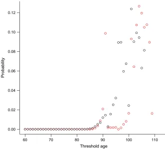
We first examine the analysis of models (6) and (8) separately. For model (6) with a log-linear mortality function at old age, the (conditional) probabilities for various threshold agesx0are displayed in Fig. 2. The probability that the transition from an unstructured (GAM) model to a parsimonious parametric form should happen at an age less than 85 years is negligible. Thereafter the parametric model becomes more competitive. For males, the total probability that a threshold is between 96 and 105 years is 0.80. For females, there is probability of around 0.1 that the threshold is at agex0=91 years but the bulk (0.81) of the total probability is on a threshold being between 101 and 108 years.
In Fig. 3, we present the model-averaged graduation for ages 60 years and older, based on model (6). This graduation incorporates uncertainty about the value of the thresholdx0by com-puting the graduated estimates by using expression (13), where the model indexk represents different values ofx0. Although models for males and females are fitted separately, the extrap-olated (log-)mortality rates are very close. In fact the extrapolation shows the rates for females overtaking those for males, but only by a very small amount relative to the overall uncertainty. Note that, although all individual models are log-linear, their average, which is calculated on the mortality scale via expression (13) is not log-linear, explaining the slight curvature in the extrapolated mortality function.
60 70 80 90 100 110 0.00
0.02 0.04 0.06 0.08 0.10 0.12
Threshold age
[image:11.485.77.408.56.355.2]Probability
Fig. 2. Threshold probabilities plotted against threshold agesx0for the log-linear old age model (6) (for each potential threshold agex0, these represent the probability thatx0is the optimal threshold at which the GAM, for mortality rates for England and Wales (2010–2012), is replaced by the log-linear old age model (6)):, males; , females
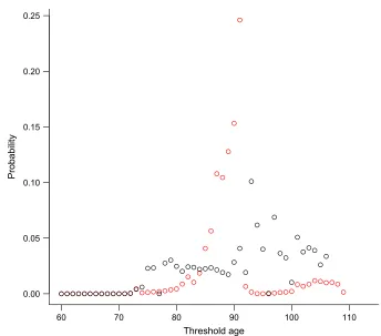
various threshold valuesx0are displayed in Fig. 4. Now, thresholds below age 85 years are more probable, although the probability that the transition from an unstructured (GAM) model to a parsimonious parametric form should happen at an age less than 70 years remains negligible. For females, there is a relatively narrow range of thresholds supported by the data, with the total probability thatx0is between 85 and 91 years estimated as 0.84. For males, in contrast, there remains considerable uncertainty about the threshold with almost all values ofx075 years having non-negligible probability. The highest probability region forx0is between 90 and 99 years, with a total probability of 0.43.
In Fig. 5, we present the model-averaged graduation for ages 60 years and older, based on model (8). As in Fig. 3, this graduation incorporates uncertainty about the value of the threshold x0by computing the graduated estimates by using expression (13), where the model indexk represents different values ofx0. Again models for males and females are fitted separately, and here there is a slightly more pronounced deviation between the extrapolated (log-)mortality rates. The extrapolation shows rates for females converging to the limiting value of 1 faster than the rates for males, resulting in a crossover. Again, the estimated differences are small and occur at ages beyond which very few data are available, and where uncertainty is greatest. It should not be taken as evidence that female mortality exceeds male mortality at the highest ages.
60 80 100 120 140 Age
Mor
tality r
ate
[image:12.485.72.406.59.357.2]10−3 10−2 10−1 1
Fig. 3. Crude central mortality rates for England and Wales (2010–2012) for ages 60 years and older, together with smooth rates estimated by a model average of old age log-linear models for various threshold agesx0: upper— , males, 2010; , males, 2011; , males, 2012; , males, smooth rates; lower— , females, 2010; , females, 2011; , females, 2012; , females, smooth rates
probabilities which quantify uncertainty both about threshold agesandabout the relative merits of the log-linear and logistic models for mortality in the highest age groups. The total probability of log-linear models (6) across all threshold agesx0is computed by using expression (16) to be 0.087 for females and 0.292 for males. Hence the data are generally more supportive of the logistic model (8) with its implied limiting mortality rate than the log-linear model of ever-increasing mortality. This is particularly so for females. For males, we remain more equivocal about the relative merits of models (6) and (8). When we estimate mortality rates by using the model-averaged combination of all the models, we obtain the estimates that are displayed in Fig. 6. Again, males and females have been fitted separately, but as shown in Fig. 3 we see convergence of estimated mortality rates until around age 120 years. Thereafter, the full model-averaged mortality rate estimates for males and females diverge, because of the greater weight on the log-linear model for males. Again, we caution against overinterpreting an extrapolation this far beyond the range of observed data.
Deceleration of mortality at older ages is an area of a vivid debate, which is intrinsically linked to a more general discussion on the limits of human lifespan and life expectancy (Olshansky
60 70 80 90 100 110 0.00
0.05 0.10 0.15 0.20 0.25
Threshold age
[image:13.485.72.416.51.354.2]Probability
Fig. 4. Threshold probabilities plotted against threshold agesx0for the logistic old age model (8) (for each potential threshold agex0, the symbols represent the probability thatx0is the optimal threshold at which the GAM, for mortality rates for England and Wales (2010–2012), is replaced by the logistic old age model (8)):
, males; , females
results that are presented in this paper for England and Wales support the deceleration hypoth-esis, at population level, albeit with a large uncertainty. Besides, the use of logistic models has an additional conceptual appeal, as they can be used to represent heterogeneity within cohorts that is caused by differences in individual frailty (Pitacco, 2016). Furthermore, our approach also allows for being agnostic about the pace of deceleration for both sexes, as it lets the data determine the deceleration rates in a given population. Generally, we believe that Fig. 6 repre-sents a graduation which provides an acceptable compromise between models (6) and (8) and between models with different threshold agesx0.
The graduated rates in Fig. 6 are presented without any uncertainty measure associated with them. This is simply because the standard life table presentation does not incorporate an uncertainty analysis. However, we consider that extending the methodology that is described here to provide uncertainty intervals is a valuable extension of the current approach and takes advantage of our Bayesian model specification. This is especially important in regions where we have sparse data, e.g. at older ages, as point estimates for these ages do not reflect the uncertainty in estimation.
60 80 100 120 140 Age
Mor
tality r
ate
[image:14.485.72.405.62.357.2]10−3 10−2 10−1 1
Fig. 5. Crude central mortality rates for England and Wales (2010–2012) for ages 60 years and older, together with smooth rates estimated by a model average of old age logistic models for various threshold agesx0: upper— , males, 2010; , males, 2011; , males, 2012; , males, smooth rates; lower— , females, 2010; , females, 2011; , females, 2012; , females, smooth rates
with model probabilities given by expression (16). Then corresponding mortality rates{m.j/x } are sampled from their conditional (given modelk.j/) posterior distribution, so
m.j/
x |k.j/,y∼p.mx|k.j/,y/:
In computing the model-averaged mortality estimates in expression (17), we use a series of approximations. Here, we sample from an approximate posterior distribution, which is a normal distribution for log.mx/with mean log.mˆ.k/x /, the (penalized) MLEs ofmxunder modelk, and standard deviation ˆσ.k/x , the predictive standard error of log.mˆx/under modelk. Hence, we use the approximation
log.mx/∼N{log.mˆ.k/x /,.σˆ.k/x /2} under modelk.
60 80 100 120 140 Age
Mor
tality r
ate
[image:15.485.79.412.59.357.2]10−3 10−2 10−1 1
Fig. 6. Crude central mortality rates for England and Wales (2010–2012) for ages 60 years and older, together with smooth rates estimated by a model average of old age logistic and log-linear models for various threshold agesx0: upper— , males, 2010; , males, 2011; , males, 2012; , males, smooth rates; lower— , females, 2010; , females, 2011; , females, 2012; , females, smooth rates
model (7), for agesx < x0. Hence, uncertainty is quantified by simple computation involving only generation from a discrete distribution over the model space, together with generating normal variables with means and standard deviations given by the outputs of the standard statistical procedures that are used to estimate mortality under each model. As the method does not involve exact computation of the posterior distributionsp.mx|k,y/, computation is much more straightforward than under the fully Bayesian approach. Similarly, a parametric bootstrap, which would require carrying out multiple repetitions of the complete analysis on resampled death counts, would be computationally much more demanding. In the analysis below, we use a simulation sample size of 100 000.
0 20 40 60 80 100 120 Age
Mor
tality r
ate
10−4
10−3
10−2
10−1
1
80 90 100 110 120 10−1
[image:16.485.46.438.72.388.2]1
Fig. 7. Smooth mortality rates estimated by a model average of old age logistic and log-linear models for England and Wales (2010–2012) for various threshold agesx0together with the 90% probability interval for smooth rates (the inset additionally shows crude central mortality rates for England and Wales (2010–2012) for ages 80 years and older): upper— , males, 2010; , males, 2011; , males, 2012; , males, smooth rates; , males, 90% probability interval; lower— , females, 2010; , females, 2011; , females, 2012;
, females, smooth rates; , females, 90% probability interval
5. The life table
The key component of the life tables is the valueslx, which represent the expected number of survivors to exact agexfrom a birth population of sizel0=100 000. Thelxare derived indirectly, from the mortality ratesmx, viaqx, which represent the conditional probability of death before exact agex+1 given survival to exact agex. The relationship betweenlandqis straightforward to derive as
lx=l0 x−1
z=0
.1−qz/, x=1, 2,: : : :
mortality rates vary sufficiently smoothly with age that this is a reasonable approximation, and an approximation which we strongly prefer to the alternative of assuming a piecewise linear survival function in each [x,x+1/, which typically implies a non-monotonic hazard at high ages.
We have already shown thatmx, given in model (1), can be expressed in terms ofμ as in model (2). Therefore the computation ofqxby using graduatedmxis now straightforward, as the standard relationship between (constant) hazard and survival function gives
qx=1−exp{−μ.x+12/} =1−exp.−mx/:
As is conventional, life table columns are presented for ages for whichl0:5. For the 17th ELTs, this required extrapolation of mortality rates to ages 114 years for females and 112 years for males. Clearly, this extrapolation goes well beyond the highest age at which we might reasonably extrapolate a semiparametric smoothing model, such as a GAM. In producing the 17th ELTs, we have made one small adjustment to the graduated rates that are provided by expression (17). The graduated estimates give a negligible positive difference between rates for females and males over a very narrow age range (112–115 years). Hence, the final entry of the life table for males (at age 112 years) would show a lower mortality (in the fourth decimal place) than the corresponding value for females. We have chosen to report the same value (based on the female graduation) at age 112 years for males and females. The final graduated life tables, the 17th ELTs, are available from Office for National Statistics (2015).
6. Conclusions
In this paper we have developed a method of graduation which takes advantage of the ease with which a wide range of smooth and parametric models can routinely be fitted, while acknowl-edging that in regions of sparse data there remains considerable uncertainty about the model which should be used to estimate and extrapolate the mortality rates. This uncertainty should be incorporated in estimation and this approach provides a computationally straightforward approach for achieving this.
In the literature review we pointed out that the history of modelling mortality as a function of age primarily uses non-parametric models for smoothing. This reflects the fact that mortality is not a simple function of age across the whole range of ages. The simplest way of graduating mortality rates would be to use a GAM over the whole age range; however, this raises the question of how to extrapolate the rates where the data are sparse. The approach that is described in this paper provides therefore a straightforward and coherent way of accurately and smoothly estimating mortality rates across the whole age range, including older ages where data are sparse or non-existent. This is naturally more complex than a single GAM, but with the benefit of not overfitting the extra variability at higher ages.
The issue with the older age groups is not poor quality of data in the sense of data in-accuracies, but more that the observed numbers of deaths are low because of low exposures (population numbers) at these ages. Hence, there is greater natural (random) variability of the observed (crude) log-mortality rates at those ages. At these ages, there is the potential for com-plex smoothing models to overfit this extra variability. Where this becomes an issue, there is a robustness–efficiency trade-off, which makes a simple parametric model a better choice. A sim-pler model allows greater borrowing of strength across ages, which is important in the regions of sparse data.
smoothing and simple parametric models is optimal, based on how well the resulting model would predict unobserved mortality rates. Furthermore, our (partial) Bayesian approach allows uncertainty about the threshold position to be coherently incorporated, so that the resulting estimates are smooth. One other way of doing this would be to use a full Bayes model. However, compared with the full Bayes method, our approach is very simple and computationally very cheap as it requires no Markov chain Monte Carlo sampling and we use pre-existing R functions. R code for the analyses in this paper is available from
http://wileyonlinelibrary.com/journal/rss-datasets
Acknowledgements
The majority of this work was supported through a research contract between the Office for National Statistics and the University of Southampton with additional support from the Eco-nomic and Social Research Council Centre for Population Change—phase II (ES/K007394/1). The views that are presented in the paper are those of the authors and do not necessarily reflect the views of the Office for National Statistics. We are grateful to the three reviewers for their comments, which have improved the earlier draft. Any remaining errors are ours.
References
Andreev, K., Jdanov, D., Soroko, E. and Shkolnikov, V. (2003) Kannisto-Thatcher database on old age mortality at the Max Planck Institute for Demographic Research: Methodology. Max Planck Institute for Demographic
Research, Rostock. (Available from http://www.demogr.mpg.de/databases/ktdb/xservices/
method.htm.)
Anson, J. (1991) Model mortality patterns: a parametric evaluation.Popln Stud.,45, 137–153.
Beard, R. E. (1963) A theory of mortality based on actuarial, biological, and medical considerations. InProc. Int.
Population Conf., vol. 1, pp. 611–625. New York: International Union for the Scientific Study of Population.
Brass, W. (1971) On the scale of mortality. InBiological Aspects of Demography(ed. W. Brass), pp. 69–110. London:
Taylor and Francis.
Carlin, B. P., Gelfand, A. E. and Smith, A. F. M. (1992) Hierarchical Bayesian analysis of changepoint problems. Appl. Statist.,41, 389–405.
Chakrabarti, A. and Ghosh, J. K. (2007) Some aspects of Bayesian model selection for prediction.Baysn Statist.,
8, 51–90.
Coale, A. J. and Demeny, P. G. (1966)Regional Model Life Tables and Stable Populations. Princeton: Princeton
University Press.
Dellaportas, P., Smith, A. F. M. and Stavropoulos, P. (2001) Bayesian analysis of mortality data.J. R. Statist. Soc.
A,164, 275–291.
Eklund, J. and Karlsson, S. (2007) Forecast combination and model averaging using predictive measures.Econmetr.
Rev.,26, 329–363.
Feldkircher, M. (2012) Forecast combination and bayesian model averaging: a prior sensitivity analysis.J.
Fore-cast.,31, 361–376.
Gallop, A. (2002) Mortality at advanced ages in the United Kingdom. InLiving to 100 and Beyond: Survival at
Advanced Ages. London: Society of Actuaries
Ghosh, P., Basu, S. and Tiwari, R. C. (2009) Bayesian analysis of cancer rates from SEER program using parametric
and semiparametric joinpoint regression models.J. Am. Statist. Ass.,104, 439–452.
Gompertz, B. (1825) On the nature of the function expressive of the law of human mortality, and on a new mode
of determining the value of life contingencies.Phil. Trans. R. Soc. Lond.,115, 513–583.
Haberman, S. and Olivieri, A. (2014) Risk classification/life.Wiley StatsRef: Statistics Reference Online. Hoboken:
Wiley.
Heligman, L. and Pollard, J. H. (1980) The age pattern of mortality.J. Inst. Act.,107, 49–80.
Hoeting, J. A., Madigan, D., Raftery, A. E. and Volinsky, C. T. (1999) Bayesian model averaging: a tutorial. Statist. Sci.,14, 382–401.
Hsieh, J. J. (1991) A general theory of life table construction and a precise abridged life table method.Biometr. J.,
33, 143–162.
Kostaki, A. (1992) A nine-parameter version of the Heligman-Pollard formula.Math. Popln Stud.,3, 277–288.
Manton, K. G., Stallard, E. and Vaupel, J. W. (1986) Alternative models for the heterogeneity of mortality risks
among the aged.J. Am. Statist. Ass.,81, 635–644.
Murray, C. J., Ferguson, B. D., Lopez, A. D., Guillot, M., Salomon, J. A. and Ahmad, O. (2003) Modified logit
life table system: principles, empirical validation, and application.Popln Stud.,57, 165–182.
Oeppen, J. and Vaupel, J. W. (2002) Broken limits to life expectancy.Science,296, 1029–1031.
Office for National Statistics (2009)English Life Tables No. 16: Methodology, 2000-02. Newport: Office for National
Statistics.
Office for National Statistics (2015)Decennial Life Tables: English Life Tables, No. 17, 2010-12. Newport: Office
for National Statistics. (Available fromhttps://tinyurl.com/ELT17.)
O’Hagan, A. and Forster, J. J. (2004)Bayesian Inference: Kendall’s Advanced Theory of Statistics, vol. 2B. London:
Arnold.
Olshansky, S. J. and Carnes, B. A. (1997) Ever since Gompertz.Demography,34, 1–15.
Olshansky, S. J., Carnes, B. A. and Cassel, C. (1990) In search of Methuselah: estimating the upper limits to
human longevity.Science,250, 634–640.
Perks, W. (1932) On some experiments in the graduation of mortality statistics.J. Inst. Act.,63, 12–57.
Pitacco, E. (2016) High age mortality and frailty: some remarks and hints for actuarial modeling.Working Paper
2016/19. Australian Research Council Centre of Excellence in Population Ageing Research, University of New South Wales, Sydney.
Pollard, J. H. and Valkovics, E. J. (1992) The Gompertz distribution and its applications.Genus,48, 15–28.
Tabeau, E., Willekens, F. and van Poppel, F. (2002) Parameterisation as a tool in analysing age, period and cohort
effects on mortality: a case study of the Netherlands. InThe Life Table: European Studies of Population, vol. 11
(eds G. Wunsch, M. Mouchart and J. Duchˆene). Dordrecht: Springer.
Thatcher, A. R. (1999) The long-term pattern of adult mortality and the highest attained age (with discussion). J. R. Statist. Soc.A,162, 5–43.
Thatcher, A. R., Kannisto, V. and Vaupel, J. W. (1998)The Force of Mortality at Ages 80 to 120. Odense: Odense
University Press.
Thiele, T. (1871) On a mathematical formula to express the rate of mortality throughout the whole of life.J. Inst.
Act.,16, 313–329.
United Nations (1982)Model Life Tables for Developing Countries. New York: United Nations Population
Divi-sion.
United Nations (1983)Manual X: Indirect Techniques for Demographic Estimation. New York: United Nations
Population Division.
Vaupel, J. W., Manton, K. G. and Stallard, E. (1979) The impact of heterogeneity in individual frailty on the
dynamics of mortality.Demography,16, 439–454.
Wilmoth, J. R., Andreev, K., Jdanov, D., Glei, D. A., Boe, C., Bubenheim, M., Philipov, D., Shkolnikov, V. and Vachon, P. (2007) Methods protocol for the human mortality database. University of California, Berkeley, and
Max Planck Institute for Demographic Research, Rostock. (Available fromhttp://mortality.org.)
Wood, S. (2006)Generalized Additive Models: an Introduction with R. Boca Raton: CRC Press.
Wood, S. (2015) Package ‘mgcv’. Department of Statistics, University of Bath, Bath. (Available fromhttp://