Dispersion in Closed, O
ff
-Axis Orbit Bumps
R. Apsimona,b, J. Esbergc, H. Owenb,d
aThe University of Lancaster, Lancaster LA1 4YW, United Kingdom
bThe Cockcroft Institute, Sci-Tech Daresbury, Daresbury, Warrington, United Kingdom
cCERN, Meyrin, Switzerland
dThe University of Manchester, Manchester M13 9PL, United Kingdom
Abstract
In this paper we present a proof to show that there exists no system of linear or nonlinear optics which can simultaneously close
multiple local orbit bumps and dispersion through a single beam transport region. The second combiner ring in the CLIC drive
beam recombination system, CR2, is used as an example of where such conditions are necessary. We determine the properties of a
lattice which is capable of closing the local orbit bumps and dispersion and show that all resulting solutions are either unphysical
or trivial.
Keywords: Dispersion; Orbit bump; Off-axis; Beam dynamics
1. Introduction
1
Typical local orbit bumps in beam transport systems vary on
2
the timescale of 0.1-100 s and therefore may use conventional
3
dipole magnets. Faster orbit bumps can be achieved with the
4
use of kicker magnets which may operate on timescales from
5
10 ns up to 100 ms. Such systems can be designed to
cor-6
rect the dispersion function either side of the local orbit bump
7
with relative ease. For some applications, such as the injection
8
into the second combiner ring CR2 for the CLIC drive beam
9
recombination system, multiple local orbit bumps are required
10
on sub-nanosecond timescales; thus RF deflectors are required
11
rather than conventional dipole magnets or kicker magnets.
12
The CLIC drive beam requires 2×24 pulses, each consisting
13
of 2904 bunches with a bunch spacing of 82 ps. To achieve this,
14
the CLIC drive beam linac produces 24×24 sub-pulses with a
15
bunch spacing of 2 ns. A recombination system is used to
inter-16
leave bunches over 3 stages to produce the required pulse trains
[image:1.595.309.562.459.634.2]17
(Figure 1). Further details of this system can be found in [1].
18
The second combiner ring stores bunch trains for up to 3.5
19
turns; on each turn an additional bunch train is injected such
20
that the bunches are interleaved with the stored bunches. The
21
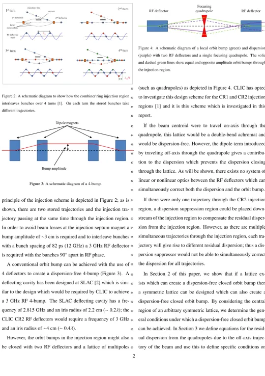
Figure 1: A schematic diagram of the CLIC drive beam recombination system
Figure 2: A schematic diagram to show how the combiner ring injection region
interleaves bunches over 4 turns [1]. On each turn the stored bunches take
different trajectories.
Figure 3: A schematic diagram of a 4-bump.
principle of the injection scheme is depicted in Figure 2; as is
22
shown, there are two stored trajectories and the injection
tra-23
jectory passing at the same time through the injection region.
24
In order to avoid beam losses at the injection septum magnet a
25
bump amplitude of∼3 cm is required and to interleave bunches
26
with a bunch spacing of 82 ps (12 GHz) a 3 GHz RF deflector
27
is required with the bunches 90◦apart in RF phase.
28
A conventional orbit bump can be achieved with the use of
29
4 deflectors to create a dispersion-free 4-bump (Figure 3). A
30
deflecting cavity has been designed at SLAC [2] which is
sim-31
ilar to the design which would be required by CLIC to achieve
32
a 3 GHz RF 4-bump. The SLAC deflecting cavity has a
fre-33
quency of 2.815 GHz and an iris radius of 2.2 cm (∼0.2λ); the
34
CLIC CR2 RF deflectors would require a frequency of 3 GHz
35
and an iris radius of∼4 cm (∼0.4λ).
36
However, the orbit bumps in the injection region might also
37
be closed with two RF deflectors and a lattice of multipoles
38
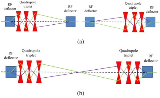
Figure 4: A schematic diagram of a local orbit bump (green) and dispersion
(purple) with two RF deflectors and a single focusing quadrupole. The solid
and dashed green lines show equal and opposite amplitude orbit bumps through
the injection region.
(such as quadrupoles) as depicted in Figure 4. CLIC has opted
39
to investigate this design scheme for the CR1 and CR2 injection
40
regions [1] and it is this scheme which is investigated in this
41
report.
42
If the beam centroid were to travel on-axis through the
43
quadrupole, this lattice would be a double-bend achromat and
44
would be dispersion-free. However, the dipole term introduced
45
by traveling off-axis through the quadrupole gives a
contribu-46
tion to the dispersion which prevents the dispersion closing
47
through the lattice. As will be shown, there exists no system of
48
linear or nonlinear optics between the RF deflectors which can
49
simultaneously correct both the dispersion and the orbit bump.
50
If there were only one trajectory through the CR2 injection
51
region, a dispersion suppression region could be placed
down-52
stream of the injection region to compensate the residual
disper-53
sion from the injection region. However, as there are multiple
54
simultaneous trajectories through the injection region, each
tra-55
jectory will give rise to different residual dispersion; thus a
dis-56
persion suppressor would not be able to simultaneously correct
57
the dispersion for all trajectories.
58
In Section 2 of this paper, we show that if a lattice
ex-59
ists which can create a dispersion-free closed orbit bump then
60
a symmetric lattice can be designed which can also create a
61
dispersion-free closed orbit bump. By considering the central
62
region of an arbitrary symmetric lattice, we determine the
gen-63
eral conditions under which a dispersion-free closed orbit bump
64
can be achieved. In Section 3 we define equations for the
resid-65
ual dispersion from the quadrupoles due to the off-axis
trajec-66
tory of the beam and use this to define specific conditions on
[image:2.595.32.559.83.783.2](a)
[image:3.595.318.556.76.257.2](b)
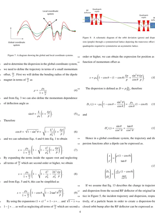
Figure 5: Diagrams illustrating the orbit deviation (green) and dispersion
(pur-ple) to show that the reflection of an asymmetric solution is also a solution (a)
and that the two can be joined to form a symmetrised solution (b).
the lattice parameters for a dispersion-free closed orbit bump
68
to exist. In Section 4 we investigate the specific conditions
un-69
der which a dispersion-free closed orbit bump may exist and
70
show that these lead to solutions which are either unphysical
71
or trivial, thus showing that no solution exists for a linear
lat-72
tice. In Section 5 we consider a non-linear lattice and show that
73
the results from Section 4 imply that no solution exists for a
74
non-linear solution either.
75
2. Requirements for a linear solution
76
2.1. Symmeterisation of an arbitrary lattice 77
If we consider an arbitrary lattice which is able to create a
78
dispersion-free closed orbit bump then by symmetry the
reflec-79
tion of this lattice must also create a dispersion-free closed
or-80
bit bump (Figure 5a). By combining the original lattice and its
81
reflection and removing the central RF deflectors, a new
lat-82
tice can be created which is symmetric and able to create a
83
dispersion-free closed orbit bump (Figure 5b). We define this
84
new lattice as the symmeterised lattice [3].
85
In order to correctly form the symmeterised lattice from the
86
original lattice, there is a transverse offset between the elements
87
in the two halves of the symmeterised lattice, as depicted in
88
Figure 8. To explain the origin of this transverse offset, we
89
should first derive expressions for the trajectory and dispersion
90
Figure 6: A diagram of the trajectory through a dipole field for a reference
particle (black) and an off-momentum particle (red).
functions due to a dipole. From figure 6 it can be shown that
91
the trajectory after the dipole is
92
x
x0
=
ρ(1−cosθ)
tanθ
, (1)
where ρ is the radius of curvature of a particle through the
93
dipole field andθis the deflection angle.
94
The dispersion through a sector bend dipole is often
ex-95
pressed as [4]
96
Dx
D0
x
=−
ρ(1−cosθ)
sinθ
, (2)
however, this expression provides the dispersion in terms of the
97
local (curvilinear) coordinate system where longitudinal axis,
98
S, is the tangent of the reference orbit at some point. We need
99
to determine the dispersion in terms of a global coordinate
sys-100
tem where the longitudinal axis,z, is fixed because this is the
101
coordinate system that the trajectory is determined in for Eq. 1.
102
Figure 7 shows the difference between the local and global
co-103
ordinate systems.
104
In the global coordinate system, the length of the dipole can
105
be expressed in terms ofρandθas
106
[image:3.595.42.303.84.243.2]Figure 7: A diagram showing the global and local coordinate systems.
and to determine the dispersion in the global coordinate system,
107
we need to define the trajectory in terms of a small momentum
108
offset, δpp. First we will define the bending radius of the dipole
109
magnet in terms of δpp as
110
ρ= ρ0
1+δpp (4)
and from Eq. 3 we can also define the momentum dependence
111
of deflection angle as
112
sinθ= L
ρ0 1+
δp p
!
. (5)
Therefore
113
cosθ= p1−sin2θ=
s
1−L
2
ρ2 0
1+δp
p
!2
(6)
and we can substitute Eqs. 4 and 6 into Eq. 1 to obtain
114
x= ρ0
1+δpp
1−
s
1−L
2
ρ2 0
1+δp
p
!2
. (7)
By expanding the terms inside the square root and neglecting
115
all terms of δpp which are second order or higher, we obtain
116
x= ρ0
1+δpp
1−
s
1−L
2
ρ2 0
−2L
2
ρ2 0
δp p
. (8)
and from Eqs. 5 and 6, this can be simplified as
117
x= ρ0
1+δpp
1−cosθ
s
1−2 tan2θδp
p
. (9)
By using the expansions (1+x)−1 =1−x+. . .and
√
1−x=
118
1−2x+. . .as well as neglecting all terms ofδpp which are second
[image:4.595.25.553.56.817.2]119
Figure 8: A schematic diagram of the orbit deviation (green) and
disper-sion (purple) through a symmeterised lattice depicting the transverse offset in
quadrupoles required to symmeterise an asymmetric lattice.
order or higher, we can obtain the expression for position as a
120
function of momentum offset as
121
x=ρ0 1−cosθ−(1−cosθ)δp
p +
sin2θ cosθ
δp p
!
. (10)
The dispersion is defined asD=p∂δp∂x, therefore
122
Dx(z)=−ρ0 1−cosθ− sin2θ
cosθ
!
= ρ0
cosθ(1−cosθ) (11)
and
123
D0x(z)=
sinθ cos3θ =
tanθ
cos2θ. (12)
Hence in a global coordinate system, the trajectory and
dis-124
persion functions after a dipole can be expressed as.
125
x
x0
=
ρ(1−cosθ)
tanθ
Dx
D0x
=
ρ
cosθ(1−cosθ) tanθ cos2θ
(13)
If we assume that Eq. 13 describes the change in trajectory
126
and dispersion from the second RF deflector of the original
lat-127
tice in Figure 5, the incident trajectory and dispersion,
respec-128
tively, of a particle beam in order to create a dispersion-free
129
closed orbit bump after the RF deflector can be expressed as
Figure 9: A schematic diagram of the orbit deviation (green) and
disper-sion (purple) through a symmeterised lattice depicting the transverse offset in
quadrupoles required to symmeterise an asymmetric lattice.
x0 x0 0 =
ρ(1−cosθ)
−tanθ
Dx
D0x
= ρ
cosθ(1−cosθ)
−costan2θθ . (14)
Figure 9 shows that if the dipole is replaced with a drift space,
131
x=0 andDx=0 occur at different locations. We can determine
132
the lengths,LxandLD, forx=0 andDx=0 respectively as
133
Lx=−x0
x0
0 =
ρ(1−cosθ) tanθ
LD=−Dx,0
D0 x,0 =
ρcos2θ(1−cosθ)
tanθcosθ =Lxcosθ
. (15)
If we replace the central RF deflectors in the symmeterised
134
lattice (Figure 5b) with drift lengths LD then the dispersion
135
Dx = 0 in the centre of the lattice as required, but the
trajec-136
tory has an offsetx=x0(1−cosθ)=ρ(1−cosθ)2. Therefore
137
if the elements in the first half of the lattice are given a
trans-138
verse offset of −ρ(1−cosθ)2 relative to the longitudinal axis
139
of symmetry and the elements in the second half of the lattice
140
are given a transverse offset ofρ(1−cosθ)2 thenx=Dx =0
141
at the midpoint of the lattice as required.
[image:5.595.50.558.78.468.2]142
Figure 10: Diagrams to show the central region for a symmeterised lattice.
2.2. Central region 143
Having shown that a symmetric lattice must exist if any
so-144
lution exists, we are able to greatly simplify the problem. By
145
applying the symmeterisation technique described above to an
146
arbitrary lattice, the trajectory and dispersion must form odd
147
functions about the midpoint of the symmeterised lattice. We
148
shall define the ‘central region’ as the symmetric doublet at the
149
centre of the symmeterised lattice as depicted in Figure 10.
150
In order to obtain an odd function through the central
re-151
gion for the trajectory and dispersion, we require the
follow-152
ing boundary conditions to be satisfied, where the subscripts 0
153
and 1 represents the initial and final states respectively for the
154
trajectory and dispersion functions.
155 x1
x01
=
−x0
x00
Dx,1 D0 x,1 =
−Dx,0
D0 x,0 . (16)
We define the transfer matrix through the central region asN,
156
where detN=1. Therefore
157 x1
x01
=
N11 N12
N21 N22
x0
x00
Dx,1
D0 x,1 =
N11 N12
N21 N22
Dx,0
D0 x,0 + Ddoub D0 doub (17)
whereDdoub andD0doub are the residual dispersion and deriva-158
tive introduced by the off-axis trajectory of the beam through
159
the quadrupoles; these terms will be defined explicitely in
Sec-160
tion 4. From Eqs. 16 and 17, we can define simultaneous
tions which must be satisfied for the trajectory to form an odd
162
function through the central region.
163
x0=−
N12 1+N11
x00
x0= 1−N22
N21
x00
(18)
The simultaneous equations in Eq. 18 describe two lines
164
which intersect at the point x0 = x00 = 0, which is a trivial
165
solution. In order for non-trivial solutions to exist, we require
166
that the two lines are equivalent, thus we obtain
167
detN=1+N11−N22. (19)
Since detN=1, we obtain the constraintN11=N22in order
168
to satify the condition on trajectory from Eq. 16. For the
disper-169
sion function, from Eqs. 16 and 18 we obtain the simultaneous
170
equations
171
Dx,0=
x0
x00D
0
x,0−
Ddoub
1+N11
Dx,0=
x0
x00D
0
x,0−
D0
doub
N21
. (20)
Therefore in order to create a dispersion-free closed orbit
172
bump the following condition must be satified.
173
N21Ddoub−(1+N11)D0doub =0. (21)
3. Calculation of residual dispersion
174
In order to determine whether a closed orbit bump through a
175
symmeterised lattice can be designed to be dispersion-free we
176
must evaluate Eq. 21 in terms of lattice parameters and
deter-177
mine under which conditions such a solution may exist. We
178
define the transfer matrix for the quadrupoles asMand remind
179
the reader that the transfer matrices for a focussing and
defo-180
cussing quadrupole respectively can be expressed as
181
Mf =
cos pkflq
sin
√
kflq
√
kf
−p
kfsin
p
kflq
cos pkflq
Md=
cosh√kdlq sinh(
√
kdlq)
√
kd √
kdsinh
√
kdlq
cosh√kdlq
(22)
and the transfer matrix,P, for a drift length,Ldr, as
182
P=
1 Ldr
0 1
. (23)
The transfer matrix, N, for the quadrupole doublet can be
183
expressed as
184
N= 2M2
11+LdrM11M21−1 (LdrM11+2M12)M11
(LdrM21+2M11)M21 2M211+LdrM11M21−1
. (24)
The residual dispersion and derivative due to the off-axis
185
beam trajectory through a quadrupole can be expressed as [4]
186
Dq=M12
lq
Z lq
0
M11(s)
ρ(s) ds−M11
lq
Z lq
0
M12(s) ρ(s) ds
D0q=M22
lq
Z lq
0
M11(s)
ρ(s) ds−M21
lq
Z lq
0
M12(s) ρ(s) ds
.
(25)
Whereρ(s) can be expressed as[3]
187
ρ(s)=∓
1+M21x0+M22x00
2 3 2
kM11x0+M12x00
. (26)
Where the∓symbol represents the sign due to a focusing
188
or defocusing quadrupole. By substituting the matrix elements
189
from Eq. 24 and using the angle sum identities for trigonometric
190
and hyperbolic functions, Eq. 25 can be simplified and used to
191
describe the residual dispersion and its derivative through the
192
first quadrupole in the central region as
193
Dq1=
Z lq
0
M12
lq−s
ρ(s) ds
D0q1=
Z lq
0
M11
lq−s
ρ(s) ds
. (27)
As the trajectory through the central region is an odd
func-194
tion about the midpoint of the lattice, the trajectory through the
195
second quadrupole has the opposite sign to the first quadrupole
196
thus the transverse deflection to the beam will have the
oppo-197
site sign and the dispersion and its derivative through the second
198
quadrupole can be expressed as
Dq2=−
Z lq
0
M12
lq−s0
ρ
lq−s0 ds 0
D0q2=− Z lq
0
M11
lq−s0
ρ
lq−s0 ds 0
. (28)
By using the change of variable s0= lq−s, the integrals in
200
Eq. 28 can be expressed as
201
− Z lq
0
Mi j
lq−s0
ρ
lq−s0 ds 0=
Z 0
lq
Mi j(s)
ρ(s) ds=−
Z lq
0
Mi j(s)
ρ(s) ds. (29)
Therefore we can expressDq1andD0q1respectively as
202
Dq1=M11
lq
Dq2−M12
lq
D0q2 D0q1=M21
lqDq2−M22
lqD0q2
. (30)
Eq. 30 can be rearranged to expressDq2andD0q2in terms of
203
Dq1andD0q1as
204
Dq2=−M11
lqDq1+M12
lqD0q1 D0q2=−M21
lqDq1+M22
lqD0q1
. (31)
The total residual dispersion and its derivative from the
cen-205
tral region is
206 Ddoub D0 doub =
M11 M12
M21 M22
1 Ldr 0 1 Dq1 D0 q1 + Dq2 D0 q2 . (32)
Substituting Eq. 31 into Eq. 32 and using the fact thatM11 =
207
M22, we can express the total residual dispersion from the
cen-208
tral region in terms of the residual dispersion from the first
209
quadrupole as
210
Ddoub=(LdrM11+2M12)D0q1
D0doub=(LdrM21+2M11)D0q1
. (33)
Substituting Eqs. 24 and 33 into Eq. 21, we obtain the
condi-211
tion for a dispersion-free closed orbit bump in terms of lattice
212
parameters.
213
−2 (LdrM21+2M11)D0q1=0 (34)
Therefore in order to create a dispersion-free closed orbit
214
bump, we require that eitherLdrM21+2M11=0 orD0q1=0.
[image:7.595.17.558.49.780.2]215
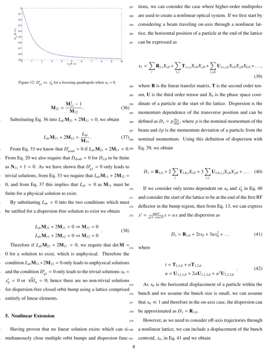
Figure 11:D0q1vs.lqfor a focusing (blue) and defocusing (red) quadrupole.
4. Results
216
4.1. D0q1=0
217
In order to determine under what conditions D0q1 = 0
oc-218
curs, Eqs. 18 and 26 are substituted into Eq. 27, the function
219
was integrated numerically in Matlab and the results shown in
220
Figure 11. For the defocusing quadrupoleD0q1increases
mono-221
tonically andD0
q1 = 0 only occurs atlq = 0 or x0 = x00 = 0,
222
which are trivial solutions. For the focusing quadrupole,
non-223
trivial solutions forD0
q1 =0 occur whenx0 =0, which implies
224
LdrM11+2M12 =0 from Eq. 18.
225
As we require x0 = 0 in order for D0q1 = 0 for a focusing
226
quadrupole, from Eq. 26,D0
q1can be expressed as
227
D0q1=− q
kfx00
Z lq
0
cos pkflq−ssin pkfs
1+x002cos2 pk
fs
32
ds (35)
wherelq = √1
kf
π−tan−1
√
kfLdr
2
!!
. Eq. 35 is an elliptic
inte-228
gral of the third kind andD0q1=0 only occurs whenx0=x00=0
229
(Figure 12) or when
√
klq = 0 (Figure 11) for a focusing
230
quadrupole, both of which are trivial solutions. Therefore there
231
are no non-trivial solutions for D0
q1 = 0 for any linear lattice
232
which can simultaneously close an off-axis orbit and dispersion
233
bump.
234
4.2. LdrM21+2M11=0
235
From Eq. 22 we can state that detM =1 andM11 =M22,
236
from which we obtain
[image:7.595.321.546.87.206.2]Figure 12:D0q1vs.x00for a focusing quadrupole whenx0=0.
M21=
M211−1
M12
. (36)
Substituting Eq. 36 intoLdrM21+2M11 =0, we obtain
238
LdrM11+2M12=
Ldr
M11
. (37)
From Eq. 33 we know thatD0
doub=0 ifLdrM21+2M11 =0.
239
From Eq. 20 we also require thatDdoub=0 forDx,0to be finite
240
asN11+1 =0. As we have shown thatD0q1 =0 only leads to
241
trivial solutions, from Eq. 33 we require thatLdrM11+2M12 =
242
0, and from Eq. 37 this implies that Ldr = 0 asM11 must be
243
finite for a physical solution to exist.
244
By substitutingLdr =0 into the two conditions which must
245
be satified for a dispersion-free solution to exist we obtain
246
LdrM21+2M11=0⇒M11 =0
LdrM11+2M12=0⇒M12 =0
. (38)
Therefore if LdrM21+2M11 = 0, we require that detM =
247
0 for a solution to exist, which is unphysical. Therefore the
248
conditionLdrM11+2M12 =0 only leads to unphysical solutions
249
and the conditionD0q1=0 only leads to the trivial solutionsx0 =
250
x00 = 0 or
√
klq = 0; hence there are no non-trivial solutions
251
for dispersion-free closed orbit bump using a lattice comprised
252
entirely of linear elements.
253
5. Nonlinear Extension
254
Having proven that no linear solution exists which can
si-255
multaneously close multiple orbit bumps and dispersion
func-256
tions, we can consider the case where higher-order multipoles
257
are used to create a nonlinear optical system. If we first start by
258
considering a beam traveling on-axis through a nonlinear
lat-259
tice, the horizontal position of a particle at the end of the lattice
260
can be expressed as
261
x1=
X
i
R1,iXi,0+
X
i,j
T1,i,jXi,0Xj,0+
X
i,j,k
U1,i,j,kXi,0Xj,0Xk,0+. . . , (39)
whereRis the linear transfer matrix,Tis the second order
ten-262
sor,Uis the third order tensor andX0 is the phase space
coor-263
dinate of a particle at the start of the lattice. Dispersion is the
264
momentum dependence of the transverse position and can be
265
defined asDx=p∂δp∂x1, wherepis the nominal momentum of the 266
beam andδpis the momentum deviation of a particle from the
267
nominal momentum. Using this definition of dispersion with
268
Eq. 39, we obtain
269
Dx=R1,6+2
X
i
T1,6,iXi,0+3
X
i,j
U1,6,i,jXi,0Xj,0+. . . (40)
If we consider only terms dependent onx0andx00in Eq. 40
270
and consider the start of the lattice to be at the end of the first RF
271
deflector in the bump region, then from Eq. 13, we can express
272
x0= tanθ
ρ(1−cosθ)x=αxand the dispersion as
273
Dx=R1,6+2tx0+3ux20+. . . (41)
where
274
t=T1,1,6+αT1,2,6
u=U1,1,1,6+2αU1,1,2,6+α2U1,2,2,6
. (42)
Asx0 is the horizontal displacement of a particle within the
275
bunch and we assume the bunch size is small, we can assume
276
thatx01 and therefore in the on-axis case, the dispersion can
277
be approximated asDx=R1,6. 278
However, as we need to consider off-axis trajectories through
279
a nonlinear lattice, we can include a displacement of the bunch
280
centroid,xb, in Eq. 41 and we obtain
Dx=R1,6+2t(x0+xb)+3u(x0+xb)2+. . . =
R1,6+2txb+3ux2b+. . .
+(2t+6uxb+. . .)x0+3ux20+. . . .
(43)
As previously stated, we assume thatx0 1, hence we can
282
neglect any terms dependent onx0 and the dispersion from an
283
off-axis trajectory becomes
284
Dx=R1,6+2txb+3ux2b+. . . (44)
where each higher order term is a perturbation to the linear
285
transfer matrix due to traveling off-axis through a higher order
286
multipole. Hence traveling off-axis through a multipole
intro-287
duces lower order multipole terms and to determine the
disper-288
sion through a nonlinear lattice, we only need to consider dipole
289
and quadrupole terms introduced. If we now consider the
mag-290
netic field experienced by a particle traveling on-axis through a
291
multipole we obtain
292
By,n= pc e knx
n
0 (45)
wheren is the order of the multipole wheren =0 is a dipole,
293
n =1 is a quadrupole and so forth. The magnetic field
experi-294
enced by a particle traveling off-axis through the multipole is
295
By,n= pcekn(x0+xb) n = pc
ekn
xn
0+nxbx
n−1
0 +. . .+nx
n−1
b x0+x n b
. (46)
By only considering the dipole and quadrupole terms from
296
Eq. 46 we obtain
297
˜ By,n= pc
enx n−1
b kn
x0+
xb n
= pc e
˜
kn
x0+
xb n
(47)
If we now consider the magnetic field experienced by the
298
beam due to traveling off-axis through a quadrupole, we obtain
299
By,2=
pc
e k2(x0+xb). (48)
By comparing Eqs. 47 and 48, we can see that traveling off
-300
axis through a higher order multipole with a horizontal
dis-301
placement xb it is equivalent to traveling off-axis through a
302
quadrupole with a horizontal displacementxb
n. As we have pre-303
viously shown that there exists no linear lattice in which a
dis-304
persion free closed off-axis orbit bump exists, hence no such
305
solution can exist in the nonlinear case either; although as the
306
order of the multipole, n, increases, the trajectory
asymptoti-307
cally converges with a closed solution.
308
As the order of the multipole increases, the dispersion
be-309
comes increasingly more strongly dependent on the beam
posi-310
tion. In a real machine it is likely that the residual dispersion
311
introduced by beam jitter would become a limiting factor on the
312
maximum order multipole that could be used in such a system.
313
6. Summary
314
In this paper we have shown that there is no possible linear
315
solution to simultaneously close orbit and dispersion functions.
316
We showed that if a solution exists then it must be possible
317
to create a symmetric lattice which is also a solution. For a
318
symmetric lattice, both the orbit and dispersion must be either
319
symmetric or anti-symmetric about the midpoint of the lattice.
320
This allows us to investigate just the central region of the lattice
321
to determine whether a solution is possible. By considering a
322
quadrupole singlet at the centre of the injection region, we are
323
able to draw conclusions about any lattice consisting of an odd
324
number of quadrupoles. Similarly by considering a doublet at
325
the centre, we are able to draw conclusions about any lattice
326
consisting of an even number of quadrupoles. By considering a
327
quadrupole singlet as the special case of a quadrupole doublet
328
with a drift lengthLdr =0, we are able to investigate all cases
329
and show that no non-trivial linear solutions exist.
330
After proving that no linear solution exists, we were able to
331
extend the proof to nonlinear optical systems. By considering
332
the multipole terms experienced by an off-axis beam and by
333
neglecting small terms, we were able to show that the lattice
334
is equivalent to traveling off-axis through a quadrupole with a
335
smaller offset. By relating this to the proof for linear optics, we
336
were able to show that no non-trivial nonlinear optics exist; thus
337
completing the proof that no solution exists to simultaneously
correct multiple local orbit bumps and dispersion functions with
339
linear or nonlinear optics.
340
Acknowledgment
341
The authors wish to thank Dr Oznur Mete-Apsimon, Dr
342
Graeme Burt and Mr Davide Gamba for their useful insight and
343
suggestions with regards to this paper.
344
References
345
[1] CLIC Collaboration, A Multi-TeV Linear Collider based on CLIC
Tech-346
nology, CLIC CDR (2012) CERN-12-007.
347
[2] V. A. Dolgashev, M. Borland and G. Waldshmidt, (2007)
SLAC-PUB-348
12955.
349
[3] R. Apsimon and J. Esberg, (2014) CLIC-Note-1035.
350
[4] H. Weidemann, Particle Accelerator Physics I: Vol. 1 (2003).
![Figure 1: A schematic diagram of the CLIC drive beam recombination system[1].](https://thumb-us.123doks.com/thumbv2/123dok_us/9411023.442327/1.595.309.562.459.634/figure-schematic-diagram-clic-drive-beam-recombination.webp)