1
A Reliability Analysis Method using BDDs in Phased Mission
Planning
*D.R. Prescott, R. Remenyte-Prescott, S. Reed, J.D. Andrews
Department of Aeronautical and Automotive Engineering, Loughborough University, Loughborough, Leicestershire, LE11 3TU, UK
C.G. Downes
BAE Systems, Warton, Preston, Lancashire, PR4 1AX, UK
*corresponding author: tel +441509227278 fax +441509227275
email [email protected]
Abstract
The use of autonomous systems is becoming increasingly common in many fields. A significant example of this is the ambition to deploy UAVs (unmanned aerial vehicles) for both civil and military applications. In order for autonomous systems such as these to operate effectively they must be capable of making decisions regarding the appropriate future course of their mission responding to changes in circumstance in as short a time as possible. The systems will typically perform phased missions and, due to the uncertain nature of the environments in which the systems operate, the mission objectives may be subject to change at short notice. The ability to evaluate the different possible mission configurations is crucial in making the right decision about the mission tasks that should be performed in order to give the highest possible probability of mission success.
Since Binary Decision Diagrams (BDD) may be quickly and accurately quantified to give measures of the system reliability it is anticipated that they are the most appropriate analysis tools to form the basis of a reliability-based prognostics methodology. This paper presents a new Binary Decision Diagram based approach for phased mission analysis, which seeks to take advantage of the proven fast analysis characteristics of the BDD and enhance it in ways which are suited to the demands of a decision making capability for autonomous systems. The BDD approach presented allows BDDs representing the failure causes in the different phases of a mission to be constructed quickly by treating component failures in different phases of the mission as separate variables. This allows flexibility when building mission phase failure BDDs since a global variable ordering scheme is not required. An alternative representation of component states in time intervals allows the dependencies to be efficiently dealt with during the quantification process. Nodes in the BDD can represent components with any number of failure modes or factors external to the system that could affect its behaviour, such as the weather. Path simplification rules and quantification rules are developed that allow the calculation of phase failure probabilities for this new BDD approach.
The proposed method provides a phased mission analysis technique that allows the rapid construction of reliability models for phased missions and, with the use of BDDs, rapid quantification.
2
1. Introduction
A phased mission is one in which a system is required to perform a number of different tasks or functions in sequence. The periods in which each of these successive tasks or functions takes place are known as phases. Each phase must be completed successfully in order that the mission can be considered a success. Many systems operate such phased missions, with aircraft being a prime example. When performing an unreliability assessment for phased mission systems failure probabilities are calculated for each of the individual phases and these are used to obtain the mission failure probability for the entire mission.
Systems whose components can undergo repair during a phased mission are known as repairable phased mission systems, whereas systems for which repair are not permitted during the mission are known as non-repairable phased mission systems. Markov techniques can deal with the dependencies introduced when repairable phased mission systems are analysed [1]. Fault tree techniques are suitable when modelling non-repairable phased mission systems since the absence of repair processes facilitates the use of such techniques that require independence [2]. Non-repairable phased missions are considered in this paper.
The size and complexity of many systems means that exact fault tree quantification is impossible and upper bounds are often used to approximate the failure probabilities. For this reason it is common to convert fault trees to Binary Decision Diagrams (BDD) before quantification takes place. The conversion process requires variables, representing fault tree basic events, to follow a specified ordering scheme and can be time-consuming for large fault trees. However, advantages are gained when converting fault trees to BDDs, since the structure of BDDs allows system failure quantification to be carried out quickly and accurately, with exact solutions being obtained without the need for approximations [3].
The BDD approach has been applied to phased mission analysis for non-repairable systems in
[4]. A fault tree is constructed, taking into account the success of previous mission phases, that represents mission failure in each phase under consideration, as well as the overall mission failure probability. In order to do this a basic event transformation, detailed in [2], is used, which replaces all basic events in a phase fault tree by a number of basic events that represent occurrence of each of the basic events in each mission phase. This results in a considerable increase in the number of basic events to be included in the analysis. The fault tree representing mission failure in the phase under consideration is then converted to a BDD, which is quantified to give an exact mission phase failure probability. In order to construct this BDD a global variable ordering scheme must be specified that encapsulates all variables in the previous successful phases as well as the phase currently considered for mission failure. This variable ordering scheme can have a significant effect on the size of the resultant BDD and, as a consequence, will affect the time taken to perform the quantification process. In [5]
a similar global variable ordering scheme is required, which then allows quantification of the overall mission failure probability, with a phase algebra being used to deal with dependencies across phases. Thus, in methods such as those in [4] and [5], if an unsuitable ordering scheme is chosen, a lengthy process of BDD construction can occur prior to quantification.
In the phased mission analysis method presented in [6] a notation is introduced for components that explicitly expresses the time periods over which components work or fail. This is used to obtain the mission failure conditions and calculate the mission failure probability. However, the method presented requires that minimal cut sets and minimal path sets be obtained, using FTA, in advance, for each phase. This requires considerable, perhaps impractical, computational effort.
3
to facilitate the use of the decision making strategy presented in [7]. A brief overview of BDDs and phased mission analysis is followed by the BDD methodology proposed to meet the challenge of providing a real-time prognostics capability within a decision making strategy. It is also described how events with multiple failure modes and external factors are incorporated in the methodology.
2. Background
2.1 Binary Decision Diagrams
Binary Decision Diagrams provide an alternative approach to fault trees to represent the failure logic of a system. BDDs can be used for the accurate quantification [8, 9] of fault trees, because exact solutions can be calculated without the requirement to evaluate minimal cut sets as an intermediate step. This method improves the accuracy and efficiency of conventional approaches [10] and is proving to be of considerable use in system reliability analysis.
2.1.1 Binary Decision Diagram Definition
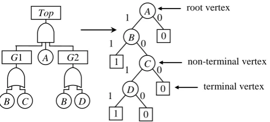
A BDD is a directed acyclic graph, where all paths through the BDD start at the root vertex and terminate in one of two states – a 1-state (system failure), or a 0-state (system success). The BDD is composed of terminal and non-terminal vertices, which are connected by branches. Terminal vertices correspond to the final state of the system and non-terminal vertices correspond to the basic events of the fault tree. By connection, all left branches leaving a vertex are the 1-branches (component fails), all right branches are the 0-branches (component functions). The construction of the BDD requires the basic events to be ordered. In Figure 1 an example fault tree is converted to a BDD with the ordering A < B < C < D. The ordering scheme employed can have a considerable effect on the number of nodes in the BDD, particularly for large fault trees. For this reason, it is important to select an ordering scheme that will minimise the size of the BDD and hence allow fast quantification.
Each path that terminates in a 1 state gives a cut set, i.e. a combination of component failure conditions where the existence of all of them will result in system failure, when only failed states of components are considered. For example, following the first path in Figure 1 gives a cut set {A, B}.
The BDD encodes the logic function of the system failure in its disjoint form, therefore, the probability of occurrence of the top event, QSYS, can be expressed as the sum of the
probabilities of the disjoint paths through the BDD. Since paths through the BDD are mutually exclusive, the probability of failure for the system in Figure 1, QSYS, is expressed as:
B
C DA B A
SYS
q
q
q
q
q
q
Q
1
. (1)4
Figure 1 - Example fault tree converted to BDD
2.1.2 Binary Decision Diagram Construction
A commonly used method of constructing BDDs was developed by Rauzy [3]. This approach applies an if-then-else (ite) technique to each of the gates in the fault tree. If f(x) is the Boolean function for the top event then the given ite structure ite(x, f1, f2) means that if
variable x occurs (fails) then consider f1, else consider f2, where f1 and f2 are Boolean
functions, known as the residues of f, with x=1 and x=0 respectively. Therefore, in the BDD structure f1 lies below the 1-branch of the node encoding x and f2 lies below the 0-branch.
First of all, a variable ordering for basic events needs to be established. Then the conversion of every gate to the BDD is performed according to the following rules. For gates whose inputs have already been defined as an ite structure the rule of the conversion process is applied, i.e. if J = ite(x, f1, f0) and H = ite(y, g1, g0) represent two inputs to a gate of logic type
, then:
ordering. the
in if
) ,
, (
ordering, the
in if
) ,
, (
0 0 1 1
0 1
y x g f g f x
y x H f H f x H
J
ite ite
(2)
The resulting BDD shown in Figure 1 is an ordered BDD, where traversing the BDD along any path from the root vertex will encounter the nodes in the order specified. Using this approach the variable ordering is retained throughout the BDD because every step of the connection is performed according to the ordering of the elements. Also, the method automatically uses sub-node sharing, storing each ite structure in the memory only once and reusing calculated ite structures further in the process.
2.2 Phased Mission Analysis
A phased mission defined in this paper has the following characteristics: A mission contains a number of consecutive and sequential phases.
A specified task has to be accomplished in each phase and therefore there are different failure criteria in each phase.
For a mission to be successful all phases must be completed successfully. The duration of each phase is known.
All components are working before the start of the mission.
The mission is non-repairable and component failures remain once they have occurred.
The phased mission is represented by a number of fault trees, each of them expressing the conditions leading to the failure of a particular phase. A method of calculating the mission failure probability is detailed in [4]. The method works by calculating the probability of failure, Qi, in each of the mission phases, i, and then adding these to give the total mission
failure probability, QMISS.
Top
G2
B D
G1
B C
A
A
1 0
1 0 B 1
C
1 0
1
0 0 D 1
0 0
root vertex
5
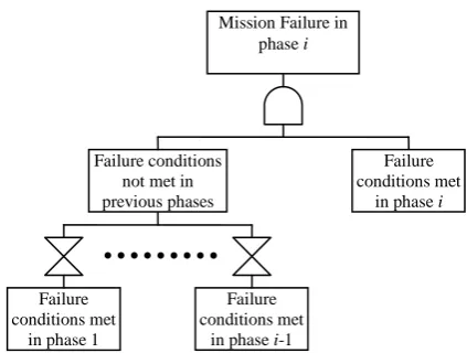
Figure 2 - Fault Tree for Mission Failure In Phase i
For any phase the method combines the causes of success of previous phases with the causes of failure for the phase being considered. The general fault tree for this is shown in Figure 2. As can be seen from the diagram, in order for the mission to fail in phase i, the failure conditions must not have been met in any of the previous i – 1 phases and then the failure conditions for phase i must be met. Let Fj represent the logical expression for the failure
conditions being met in phase j and Phj represent the logical expression for mission failure in
phase j. Then:
j j
j
F
F
F
F
F
Ph
F
F
Ph
F
Ph
1 3
2 1
2 1 2
1 1
(3)These logical expressions are represented by fault trees such as that in Figure 2. Fault tree analysis can be used to quantify the probability of mission failure during mission phase i,
ii
P
Ph
Q
. (4)The total mission failure probability is given by adding these mission phase failure probabilities:
n
i i
MISS Q
Q
1
. (5)
When efficiency and accuracy of the analysis is important, the fault trees for mission failure in phase i, representing Phi, are converted to BDDs in order to be able to accurately obtain the
probability of mission failure. This means that the logical expressions for mission failure in phase i presented in equation (3) are effectively converted to a BDD format which allows fast, efficient quantification of the mission phase failure probabilities.
3. Autonomous System Mission Planning Methodology
3.1 Motivation
The motivation behind this research is to develop a strategy for the reliability analysis of phased missions which could be used as part of a decision making capability for autonomous systems. In [7] a decision making strategy for autonomous systems is presented, for which a phased mission analysis capability is required. Since results from this phased mission analysis capability are required in order to make decisions as to how the phased mission being performed should progress, it is imperative that reliable results can be obtained in as short a time as possible.
Mission Failure in phase i
Failure conditions met
in phase 1
Failure conditions met
in phase i-1 Failure conditions
not met in previous phases
Failure conditions met
6
For example, consider a UAV that is required to perform whichever of a number of possible missions is most likely to be completed successfully. Consider also that it must autonomously make a decision as to which mission to perform in a short period of time, since the window of opportunity for performing each of the missions is small. A technique is required that allows the UAV to quickly quantify the probability of success for each of the possible missions in order to decide which mission to perform. The chosen mission will be the one with the highest probability of success.
The methodology presented here is aimed at performing a phased mission analysis in order to quantify the probability, Qi, of system failure in each of the i mission phases of a particular
mission being performed and also the probability of failure over the course of the entire mission, QMISS.
3.2 Overview
BDDs offer the potential to move towards the real-time quantitative phased mission analysis demanded by a prognostics capability in a decision making strategy. They allow fast quantification of the mission phase failure probabilities, Qi, which can then be used to
calculate the total mission failure probability, QMISS. However, considerable time can be spent
converting fault trees to BDDs, time which would severely impact on the ability to offer real-time analysis of phased mission systems. For this reason, the phased mission modelling methodology presented is focussed on reducing this construction time and having phased mission BDDs available as early as possible in order that analysis can begin soon after a mission configuration becomes known. Essentially, the idea is that certain parts of the methodology are carried out offline, before a mission configuration is known, and other parts online, once the mission configuration is known. The goal is to minimise the online processes that must take place before quantification can begin and therefore move towards a real time analysis that can be used in a decision making process. The idea is that in starting the quantification sooner it may be apparent at an earlier time whether or not the failure probability of a certain mission configuration is acceptable.
Figure 3 gives a representation of the steps involved in the phased mission analysis. These are briefly described below:
1. This step can be carried out offline, before a mission configuration is known, For any system to which the decision making capability will be applied, the failure of all possible tasks (mission phases) that can possibly be performed must be represented using fault trees. These are then converted to the BDDs that will be used to represent the failure conditions being met in each of the mission phases, Fi. The methodology
allows these BDDs to be constructed independently and thus time can be taken in choosing a suitable variable ordering scheme for each BDD that enables its size to be minimised. These BDDs will then effectively be stored in a library ready for later use. Since this step is carried out offline, as much time as is available can be taken to perform this step.
2. This is the first of the online steps, and will contribute towards the time taken to perform an analysis after a phased mission becomes known. The mission is defined in terms of a mission profile. This specifies the order of the tasks that the system is to perform and the time to be taken doing each of them. This information is applied to the appropriate BDDs from the library, resulting in BDDs representing Fi, which are
thus ready to be used to construct the BDDs for mission failure in the various mission phases, Phi. The time taken to perform this step will be minimal since it is a very
simple process, as will be described later.
3. This step is crucial in being able to begin quantitative analysis as quickly as possible. Rather than having to combine the BDDs representing Fi and follow a global variable
7
be taken into account, in constructing BDDs representing Phi, there is a simple
connection process that will take little time to perform. It requires no further variable ordering and allows rapid connection of the Fi BDDs, each of which follows its own
variable ordering scheme that was assigned during step 1 in order to attempt to minimise its own size.
4. Quantification of the Phi BDDs can begin. The calculated failure probabilities can be
monitored during the quantification process for acceptability.
[image:7.595.195.407.213.403.2]In the following sections the BDD based phased mission methodology is described in more detail. It is also described how a number of categories of variable can be dealt with using the methodology.
Figure 3 - Stages of the Methodology
3.3 Notation
In the proposed methodology there are three categories of variable that will be considered. Two of these categories are components of the system and the final one represents factors external to the system that influence its operation during the mission. Descriptions of each of these follow, along with the notation that will be used for each.
3.3.1 Single Failure Mode Variables
These variables represent components of the system that can exist in only two states, either working or failed. Each component has an indicator variable,
x
k(
t
i,
t
j)
, defined as follows:
otherwise.
,
0
,
time
to
time
from
fails
component
if
,
1
)
,
(
i j i jk
t
t
k
t
t
x
(6)where k = 1,…,nS and ns is the number of single failure mode components in the system.
When considering the success state of single failure mode variables this equivalence holds:
)
,
(
)
,
(
0 i
k i
k
t
t
x
t
x
. (7)This means that when component k does not fail from time t0 until time ti,it can fail after time
ti,, where t0 is the start time of the mission.
3.3.2 Multiple Failure Mode Variables
These variables represent components of the system that can exist in a working state or one of a number of known failed states. For example, consider a valve that can fail in an open or a closed position. Each of these components has an indicator variable defined as:
1. Phase failure logic BDD construction, Fi
2. Mission definition
3. Connect phase BDDs to give mission phase BDDs, Phi
4. Quantification, giving Qi and
QMISS
Offline:
Online:
Online:
8
otherwise.
,
0
,
mode
in
time
to
time
from
fails
component
if
,
1
)
,
(
t
t
k
t
t
l
x
i j i jl
k (8)
where k = 1,…,nM,nM being the number of multiple failure mode components in the system, l
= 1,…,m, with m being the number of failure modes of component k.
When considering multiple failure mode variables in their success state a similar equivalence to the one for single failure mode variables holds:
)
,
(
)
,
(
0 i
lk i
l
k
t
t
x
t
x
. (9)This means that when component k does not fail from time t0 until time ti in its failure mode l,
it can fail in that failure mode after time ti.
3.3.3 External Factor Variables
These variables represent factors that would appear in a system’s phase fault tree but not be a part of the system. Examples of such factors are an electrical storm or rain that could affect the performance of an aircraft. The indicator variable for these factors is defined as:
otherwise.
,
0
,
time
to
time
from
appears
factor
external
if
,
1
)
,
(
i j i je k
t
t
k
t
t
x
(10)where k = 1,…,nE and nE is the number of external factors.
3.4 Methodology Steps
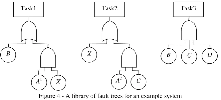
[image:8.595.108.488.477.650.2]The methodology involves a number of steps, given that fault trees are known for all of the possible phases that can be performed by the system. These fault trees will represent certain tasks or functions that the system can perform. A number of these are configured in sequence in order to fulfil the requirements of a mission. Note that, as the methodology is described here, the mission configuration for the system is initially unknown, i.e. the ordering and length of phases is not yet determined. The steps in the methodology are described in the following subsections. Each step will be applied to an example system, which can perform 3 possible tasks, represented by the fault trees shown in Figure 4.
Figure 4 - A library of fault trees for an example system
A number of basic events appear in the fault trees for the example system: basic events A, B, C and D represent system components and basic event X is an external factor that influences the behaviour of the system. All system components, except A, are single failure mode components, and component A can fail in two modes, i.e. A1 and A2.
A1 X
Task3
B C D
Task2
X
A2 C Task1
9
3.4.1 Convert System Phase Fault Trees to BDDs
In order to be ready to evaluate the probability of mission failure in as short a time as possible when the mission configuration is decided the fault trees for the potential mission phases, i.e. the tasks that can be performed by the system, are converted to BDDs using the techniques outlined earlier. This means that the time taken to construct the BDDs does not impinge on the time available to quantify them once the mission configuration is decided. Each BDD is converted using its own variable ordering scheme, which is chosen in order to minimise, as much as possible, the size of the BDD. The variables of the BDDs will each fall into one of the three categories outlined above (single or multiple mode failure or external factor).
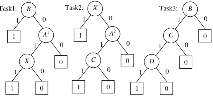
[image:9.595.126.472.296.452.2]Performing this step on the example system requires that a variable ordering be assigned to each fault tree before the fault trees are converted to BDDs. Using a simple top-down left-right traversal of basic events in the fault trees for tasks 1, 2 and 3 sets the variable ordering schemes, i.e. for Task1 – B < A1 < X, for Task2 - X < A2 < C and for Task3 – B < C < D. The BDDs obtained are shown in Figure 5. This library of BDDs is now ready to be used in the phased mission analysis as soon as the mission configuration is known.
Figure 5 - The library of BDDs representing example system tasks.
3.4.2 Mission Definition and Variable Time Association
When the mission is defined for the system the tasks or functions that must be performed, and the sequence in which they should occur, are known. The time at which each task or function will start and end is also known and this means that the phases of the mission have now been determined. Given this information it is now necessary to assign the time interval over which each of the variables contributes to phase failure for each of the phase failure logic BDDs representing Fi. Thus, each indicator variable, as defined in equations (6), (8) and (10) will
now have an associated ti and tj. These will be determined as follows for the three variable
categories:
For the single failure mode and multiple failure mode variables: ti is given by the start
time for the mission and tj by the end time for the phase with which the variable is
associated. This is because the failure of components represented by these variables can contribute to the failure of the phase at any time during the period from the start of the mission to the end of that phase.
For the external factor variables: ti and tj are given by the start and end times
respectively of the phase with which the variable is associated. This is due to the fact that whether or not the external factor occurred before the phase is not important to the failure of this phase. All that matters is whether or not the external factor occurs in that phase. For example, if one considers rain affecting a system in a certain phase, it will not matter if the rain occurred at an earlier time, only if it occurs in the phase
X
1
1
0
1
1 0
C
0 1
0 A2
0
1
1 0
D
0 1
0 C
0 1
0 B
0 Task3:
Task2: B
1
1
0
1
1 0
X
0 1
0 A1
10
under consideration. If this assumption is not true, and, for example, rain in a phase could affect the performance of the system in a later phase, then the external factor must be treated as a single failure mode variable. In this case time ti and tjare given by
the start and end times respectively of the interval when the external factor affects the system performance.
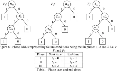
Consider the case where the example system will perform a mission consisting of three phases, where Phase I is represented by Task1, Phase II – by Task3 and Phase III – by Task2. Given this mission configuration, BDDs representing F1, F2 and F3 are selected from the BDD
library to be used in the subsequent phased mission analysis. Start and end times are assigned to each phase as shown in Table 1. Thus the time intervals over which each of the variables will contribute to phase failure is known and thus each node in the BDDs selected for the mission phases is assigned two time indices as shown in Figure 6. The BDDs in Figure 6 now encode the failure logic of each phase, taking into account the time intervals over which the variables can contribute to phase failure. That is, not only for the current phase but also for preceding phases, if appropriate. For example, for the single failure mode variables in the phase 2 BDD (F2) the state of the components in phases 1 and 2 is taken into account. The
[image:10.595.97.496.323.577.2]dependencies between related variables in different phases are taken account of during quantification.
Figure 6 - Phase BDDs representing failure conditions being met in phases 1, 2 and 3, i.e. F1,
F2 and F3
Phase Start time End time I t0 = 0 t1 = 1
II t1 = 1 t2 = 2
III t2 = 2 t3 = 3
Table1 - Phase start and end times
3.4.3 Connection of Phase Failure Logic BDDs
This step of the methodology involves building the logical expressions for mission failure in phase i, Phi, represented in equation (3) by using the appropriate BDDs for the failure
conditions being met in phase i, Fi. When using BDDs to represent Fi and times are associated
with the variables as described above the process of constructing BDDs representing Fi is
relatively simple. In order to consider the success of the mission in a certain phase the 0 and 1 terminal nodes of the BDD are swapped. This gives a dual BDD representing success in a phase. The AND connection of two BDDs, performed when building the Phi BDDs, is done
by connecting all terminal 1 nodes of one BDD to the root node of the BDD to be connected to that BDD. Although different BDDs might contain identical variables that would normally be required to adhere to a specific ordering scheme covering both BDDs, this is not the case with this method. Instead, upon connection the variables are treated as independent, with the times associated with the variables being used to take into account dependencies between them during quantification. This vastly reduces time taken to construct the mission phase
1 01
A B01
1
1
0
1
1 0
X01
0 1
0 0 F1:
2 03
A
X23
1
1
0
1
1 0
C03
0 1
0 0 F3:
1
1 0
D02
0 1
0 C02
0 1
0 B02
11
failure BDDs representing Phi, allowing fast, efficient connection of the phase BDDs
representing Fi.
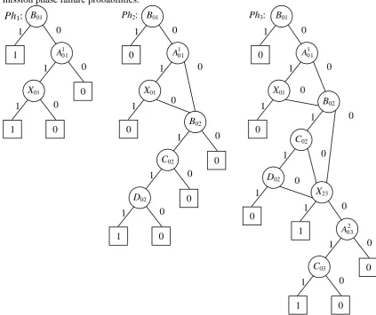
For the example mission the BDDs representing Phi, obtained after using the rules above to
connect the BDDs representing Fi as required to represent previous phase success and current
[image:11.595.87.511.155.510.2]phase failure, are shown in Figure 7. These BDDs are now ready to be quantified to obtain the mission phase failure probabilities.
Figure 7 - BDDs representing Ph1, Ph2 and Ph3
3.4.4 Phase Failure Quantification
In this step of the methodology the Phi BDDs constructed by connecting the phase failure
logic BDDs, Fi, are quantified to give the mission phase failure probabilities, as in equation
(4). The quantification process involves tracing through the BDD from the root node along all possible paths to terminal 1 nodes. Traversing the 1 branch from a node corresponds to component failure or occurrence and traversing along the 0 branch corresponds to component success or non-occurrence. When considering the success state related to a variable equations (7) and (9) are used. Since all paths are disjoint, the path probabilities are added to give the total mission phase failure probability. A general path in the BDD to be quantified will contain more than one instance of a variable due to the fact that a global variable ordering scheme for the BDDs was not required. Each instance represents the same component failure in different time intervals. Taking account of these time intervals allows dependencies between related variables in different phases to be considered. In order to allow quantification to take place a process of simplifying the path failure logic must take place as the path is traced through the BDD. This process works by performing simple calculations with the times associated with each variable encountered on the path, applying simplification rules described below. In this way, upon reaching a terminal 1 node, every variable encountered along the
1 01
A B01
1
0
0
1
0
X01 0
1 0
1
0
D02 0
1 C02
0 1
B02
0
X23
1
1
0
1
1 0
C03
0 1
0 0
2 03
A Ph3:
1 01
A B01
1
0
0
1
0 X01
0
1 0
1
1 0
D02
0 1
0 C02
0 1
0 B02
0 Ph2:
1 01
A B01
1
1
0
1
1 0
X01
0 1
12
specific path leading to that node will have associated with it a start and an end time, dependencies between variables will have been removed and quantification may take place. The time intervals within which the variables occur (given by the associated start and end times) govern the quantification process that occurs for each variable on the path as the terminal 1 node is reached. The process for the three different types of variable is given below. Once all of the probabilities have been calculated for the individual variables along the path to be quantified they are multiplied together to give the path probability.
Single Failure Mode Variables
Simplification rules applied to single failure mode variables are defined as follows:
0
)
,
(
i j
k
t
t
x
, ift
i
t
j (11))) , min( ), , (max( ) , ( ). ,
( i1 j1 k i2 j2 k i1 i2 j1 j2
k t t x t t x t t t t
x (12)
Applying these rules to a path leads to a variable xk(ti, tj) which may or may not be equal to 0.
If not, then a probability for this variable is calculated as follows:
j i t t k j ik
t
t
f
t
dt
x
P
,
1
(
)
(13)where fk(t) is the failure probability density function for component k.
This probability can then be used in the quantification of a path containing component k.
Multiple Failure Mode Variables
Two cases are presented for multiple failure mode variables, the first being when only one failure mode appears on a path and the second when more than one failure mode appears on a path.
If there is only one failure mode (out of all the possible failure modes) considered on a path equivalent rules to equations (11) and (12) are used:
0
)
,
(
i j
lk
t
t
x
, ift
i
t
j (14)))
,
min(
),
,
(max(
)
,
(
).
,
(
i1 j1 kl i2 j2 kl i1 i2 j1 j2l
k
t
t
x
t
t
x
t
t
t
t
x
(15)If two different failure modes, l1 and l2, are considered on a path l1 ≠ l2, equation (12) is
expressed as follows:
0
)
,
(
).
,
(
2 22 1 1 1
j i l k j i lk
t
t
x
t
t
x
. (16)This is due to the fact that a component cannot fail in more than one failure mode. Equation (16) is applied if
t
j1
andt
j2
.If
t
j1
andt
j2
,x
kl1(
t
i1,
t
j1)
is expressed asx
lk1(
t
0,
t
i1)
, using equation (9). Then equation (16) is expressed as given below:)
,
(
)
,
(
).
,
(
2 22 2 2 2 1 0 1 j i l k j i l k i l
k
t
t
x
t
t
x
t
t
x
. (17)
This rule is explained by the fact that if a component has failed in a particular failure mode l2
then it cannot have failed in any other failure mode.
Applying these rules to a path containing components with multiple failure modes yields a variable l
(
i,
j)
k
t
t
x
which may or may not be equal to 0. If not, then a probability for this13
Case 1 - Only one of the possible failure modes for a variable appears in the simplified path logic.
In this case the failure probability for the variable is calculated in the same way that it was for the single failure mode variable, i.e.
ji t t l k j i l
k t t f t dt
x
P , 1 ( ) (18)
where fk l
is the failure probability density function for component k in failure mode l.
Case 2 - More than one of the possible failure modes for a variable appears in the path logic.
It only occurs in situations when working states of multiple failure mode variables are considered, since the combinations of more than one failed states of the same variable have been removed using equation (16). When this occurs the failure probability for the variable is calculated as follows:
, ... , 1
.1 0 , ... , 1 , ... , 0 1 0 1 0 1 0 1 1 1 im lm k i l k im lm k i l k im lm k i l k t t x t t x P t t x t t x P t x t x P (19)
Since
x
lk1(
t
0,
t
i1)
…x
klm(
t
0,
t
im)
are mutually exclusive, i.e. component k cannot fail in more than one failure mode at the same time, this expression is equivalent to:
.
...
1
1
,
...
1
,
1
0 1 0 1 0 1 0 1
i timt lm k t t l k im lm k i l k
dt
f
dt
f
t
t
x
P
t
t
x
P
(20) External FactorsFor variables that represent external factors no rules for the simplification of paths need to be considered, since external factors occur independently in each phase. Quantification takes account of the mission phases under consideration
i je k j
i e
k
t
t
q
t
t
x
P
,
1
,
. (21)
i je k j
i e
k
t
t
q
t
t
x
P
,
1
1
,
. (22)
The BDDs representing Phi for the example system shown in Figure 7 are traversed from the
top node to each terminal 1 vertex and the paths are identified. For Phase I there are two paths:
1.
B
012.
B
1A
011X
01No simplification rules need be applied to these Phase 1 paths, since no components are represented by more than one variable in each path. In addition to this, for the variable representing the component with multiple failure modes, A101, this also appears in isolation in
the path.
For simplicity use l ij k
q
, which describes the failure probability of component k failing inmode l in time interval (ti, tj). For example, 1
01
A
q
is the probability of component A failing inits first failure mode in time interval (t0, t1). Using this terminology and the quantification
14
e X A B
B
q
q
q
q
Q
01 1 01 01 011
(
1
)
.For Phase II there also are two paths, shown below on the left. Here the simplification rule (12) is applied to a single failure mode variable
B
1B
02
B
12 leading to the two simplified expressions of the path logic shown on the right.1.
B
1A
011X
01B
02C
02D
022. 02 02 02
1 1
1
A
B
C
D
B
1.
B
12A
011X
01C
02D
022. 02 02
1 1 12
A
C
D
B
The Phase II failure probability Q2is calculated as:
02 02 1 01 12 02 02 01 1 01 12
2
(
1
)
C D B(
1
A)
C De X A
B
q
q
q
q
q
q
q
q
q
Q
.Considering Phase III there are twelve paths in the BDD for Ph3, shown on the left below.
1.
B
1A
011X
01B
02C
02D
2X
23 1.B
12A
011X
01C
02D
2X
232.
B
1A
011X
01B
02C
02D
2X
23A
032C
03 2. -3.
B
1A
011X
01B
02C
2X
23 3.B
12A
011X
01C
2X
234.
B
1A
011X
01B
02C
2X
23A
032C
03 4. -5.
B
1A
011X
01B
2X
23 5.B
2A
011X
01X
236.
B
1A
011X
01B
2X
23A
032C
03 6. -7. 02 02 2 23
1 1
1 A B C D X
B 7. 02 2 23
1 1
12A C D X
B
8. 03 2 03 23 2 02 02 1 1
1
A
B
C
D
X
A
C
B
8. 02 2 232 03
12
A
C
D
X
B
9. B1A11B02C2X23 9.
B
12A
11C
2X
2310.
B
1A
11B
02C
2X
23A
032C
03 10.B
12A
032C
23X
2311. 2 23
1 1 1 A B X
B 11. 23
1 1 2 A X
B
12. 03 2 03 23 2 1 1
1 A B X A C
B 12. 23 03
2 03 2 A X C
B
For these paths a number of simplification rules is applied. For single failure mode variables equation (12) is used to simplify
B
1B
02
B
12,B
1B
2
B
2,C
02C
03
C
02 and23 03 2
C
C
C
. For multiple failure mode variables equations (15), (16) and (17) are appliedto give 032 0
1 01A
A and 032
2 03 1 01 2 03 1
1
A
A
A
A
A
. Therefore, paths 2, 4 and 6 are seen to be zero and the others now have simplified path logic as shown on the right.The Phase III failure probability, Q3, can now be calculated in the same way that Q1 and Q2
were calculated, quantifying the probability of each path by multiplying probabilities of each component and then summing the individual path probabilities. The overall mission failure probability can then be calculated using equation (5), i.e.
3 2 1
Q
Q
Q
Q
MISS
.4. Conclusions
15
known. The quantification process involves path simplification and quantification rules that will make up the greater part of the time spent in the online implementation of the methodology. The quantification process is therefore the greatest contributor to this online implementation with the time taken increasing with the complexity of the systems and number of phases in the mission. A benefit of using this technique is that there is little time taken in constructing the mission BDD model online, regardless of the complexity of the systems or number of mission phases. The methodology involves:
Fault tree conversion to BDDs in advance of any knowledge of mission configuration.
A simple method, using component time requirements, of representing the phase of the mission in which a task is performed, which can then be used during quantification to account for phase variable dependencies.
Simple connection of the BDDs representing the logical expressions for failure conditions being met in phase i when constructing the logical expressions for mission failure in phase i. There is no need for a global ordering scheme to be applied.
The potential to minimise the size of the mission phase failure BDDs to be quantified, taking advantage of the fact that a global ordering scheme need not be followed and instead that phase failure logic BDDs may be individually minimised.
The methodology also includes rules that govern how components with multiple failure modes and variables that represent effects external to the system can be incorporated into the BDD analysis.
5. Acknowledgements
Financial support for this work has been provided by DTI, EPSRC and BAE SYSTEMS as part of the ASTRAEA (Autonomous Systems Technology Related Airborne Evaluation and Assessment) and NECTISE (Network Enabled Capability Through Innovative Systems Engineering) research programmes.
6. References
1 Smotherman, M. and Zemoudeh, K. A Non-homogeneous Markov Model for Phased Mission Reliability Analysis. IEEE Trans. Reliability,1989, vol. 38, 585-590.
2 Esary, J.D. and Ziehms, H. Reliability Analysis of Phased Missions. Reliability and Fault Tree Analysis, 1975, 213-236.
3 Rauzy, A. New Algorithms for Fault Tree Analysis. Reliability Engineering and System Safety, 1993, vol. 40, 203-211.
4 LaBand, R. and Andrews, J.D. Phased Mission Modelling Using Fault Tree Analysis. Proceedings of the IMechE, Part E: Journal of Process Mechanical Engineering, 2004, vol. 218, 83-91.
5 Zang, X., Sun, H. and Trivedi, K.S. A BDD-Based Algorithm for Reliability Analysis of Phased-Mission Systems. IEEE Transactions on Reliability, 1999, vol. 48, 50-60.
6 Kohda, T., Wada, M. and Inoue, K. A Simple Method for Phased Mission Analysis. Reliability Engineering and System Safety,1994, vol. 45, 299-309.
7 Prescott, D.R., Remenyte-Prescott, R. and Andrews, J.D. A Systems Reliability Approach to Decision Making in Autonomous Multi-Platform Missions Operating a Phased Mission. Proceedings of the Annual Reliability and Maintainability Symposium, 2008, 8-14.
8 Sinnamon, R.M. and Andrews, J.D. Improved Accuracy in Quantitative Fault Tree Analysis. Quality and Reliability Engineering International, 1997, vol. 13, 285-292.
9 Sinnamon, R.M. and Andrews, J.D. Improved Efficiency in Qualitative Fault Tree Analysis. Quality and Reliability Engineering International, 1997, vol. 13, 293-298.