Abstract— Designing generic problem solvers that perform well across a diverse set of problems is a challenging task. In this work, we propose a hyper-heuristic framework to automatically generate an effective and generic solution method by utilizing grammatical evolution. In the proposed framework, grammatical evolution is used as an online solver builder, which takes several heuristic components (e.g. different acceptance criteria and different neighborhood structures) as inputs and evolves templates of perturbation heuristics. The evolved templates are improvement heuristics which represent a complete search method to solve the problem at hand. To test the generality and the performance of the proposed method, we consider two well-known combinatorial optimization problems; exam timetabling (Carter and ITC 2007 instances) and the capacitated vehicle routing problem (Christofides and Golden instances). We demonstrate that the proposed method is competitive, if not superior, when compared to state of the art hyper-heuristics, as well as bespoke methods for these different problem domains. In order to further improve the performance of the proposed framework we utilize an adaptive memory mechanism which contains a collection of both high quality and diverse solutions and is updated during the problem solving process. Experimental results show that the grammatical evolution hyper-heuristic, with an adaptive memory, performs better than the grammatical evolution hyper-heuristic without a memory. The improved framework also outperforms some bespoke methodologies which have reported best known results for some instances in both problem domains.
Index Terms—Grammatical Evolution, Hyper-heuristics, Timetabling, Vehicle Routing
I. INTRODUCTION
ombinatorial optimization can be defined as the problem of finding the best solution(s) among all those available for a given problem [1]. These problems are encountered in many real world applications such as scheduling, production planning, routing, economic systems and management [1]. Many real world optimization problems are complex and very difficult to solve. This is due to the large,
Nasser R. Sabar and Masri Ayob are with Data Mining and Optimisation Research Group (DMO), Centre for Artificial Intelligent (CAIT), Universiti Kebangsaan Malaysia, 43600 UKM Bangi, Selangor, Malaysia.
email:[email protected], [email protected]
Graham Kendall and Rong Qu are with ASAP Research Group, School of Computer Science, The University of Nottingham, Nottingham NG8 1BB, UK.email:[email protected], [email protected]
and often heavily constrained, search spaces which make their modeling (let alone solving) a very complex task [2]. Usually, heuristic methods are used to solve these problems, as exact methods often fail to obtain an optimal solution in reasonable times. The main aim of heuristic methods, which provide no guarantee of returning an optimal solution (or even near optimal solution), is to find a reasonably good solution within a realistic amount of time [3, 4]. Meta-heuristic algorithms provide some high level control strategy in order to provide effective navigation of the search space. A vast number of meta-heuristic algorithms, and their hybridizations, have been presented to solve optimization problems. Examples of meta-heuristic algorithms include scatter search, tabu search, genetic algorithms, genetic programming, memetic algorithms, variable neighborhood search, guided local search, GRASP, ant colony optimization, simulated annealing, iterated local search, multi-start methods and parallel strategies [3],[4].
Given a problem, an interesting question that comes to mind is:
Which algorithm is the most suitable for the problem at hand and what are the optimal structures and parameter values?
The most straightforward answer to the above question might be to employ trial-and-error to find the most suitable meta-heuristic from the large variety of those available, and then employ trial-and-error to determine the appropriate structures and parameter values. While these answers seem reasonable, in terms of the computational time involved, it is impractical in many real world applications. Many bespoke meta-heuristic algorithms that have been proposed over the years are manually designed and tuned, focusing on producing good results for specific problem instances. The manually designed algorithms (customized by the user and not changed during problem solving) that have been developed over the years are problem specific, i.e. they are able to obtain high quality results for just a few problem instances, but usually fail on other instances even of the same problem and cannot be directly applied to other optimization problems. Of course, the No Free Lunch Theorem [5] states that a general search method does not exist, but it does not mean that we cannot investigate more general search algorithms to explore the limits of such an algorithm [6-8].
Numerous attempts have been made to develop automated search methodologies that are able to produce good results
Grammatical Evolution Hyper-heuristic for Combinatorial
Optimization problems
Nasser R. Sabar, Masri Ayob, Graham Kendall,
Senior Member, IEEE
and Rong Qu,
Senior
Member,
IEEE
across several problem domains and/or instances. Hyper-heuristics [6], meta-learning [9], parameter tuning [10], reactive search [11], adaptive memetic algorithms [12] and multi-method [13], are just some examples. The performance of any search method critically depends on its structures and parameter values [6]. Furthermore, different search methodologies, coupled with different structures and parameter settings may be needed to cope with problem instances or different problem domains [9],[10]. A search may even benefit from adapting as it attempts to solve a given instance. Therefore, the performance of any search method may be enhanced by automatically adjusting their structures or parameter values during the problem solving process. Thus, the ultimate goal of automated heuristic design is to develop search methodologies that are able to adjust their structures or parameter values during the problem solving process and work well, not only across different instances of the same problem, but also across a diverse set of problem domains [6], [9], [10]. Motivated by these aspects, particularly the hyper-heuristic framework [6], in this work, we propose a grammatical evolution hyper-heuristic framework (GE-HH) to generate local search templates during the problem instance solving process, as depicted in Fig 1.
Fig.1.The GE-HH framework
The evolved templates represent a complete local search method which contains the acceptance criteria of the local search algorithm (to determine away of escaping from local optima), the local search structures (neighborhoods), and their combination. The GE-HH operates on the search space of heuristic components, instead of the solution space. In addition, GE-HH also maintains a set of diverse solutions, utilizing an adaptive memory mechanism which updates the solution quality and diversity as the search progresses. We choose grammatical evolution to search the space of heuristic components due to its ability to represent heuristic components and it being able to avoid the problem of code bloat that is often encountered in traditional genetic programming. Our objectives are:
- To design an automatic algorithm that works well across different instances of the same problem and also across two different problem domains.
- To merge the strengths of different search algorithms in one framework.
- To test the generality and consistency of the proposed method on two different problem domains.
The performance and generality of the GE-HH is assessed using two well-known NP-hard combinatorial optimization problems; examination timetabling (Carter [14] and ITC 2007 [15] instances) and the capacitated vehicle routing problem (Christofides [16] and Golden [17] instances). Although both domains have been extensively studied by the research community, the reasons of choosing them are twofold. Firstly, they represent real world applications and the state of the art results, we believe, can still be improved. Currently, a variety of algorithms have achieved very good results for some
instances. However, most methodologies fail on generality and consistency. Secondly, these two domains have been widely studied in the scientific literature and we would like to evaluate our algorithm across two different domains that other researchers have studied. Although our intention is not to present an algorithm that can beat the state of the art, but rather can work well across different domains, our results demonstrate that GE-HH is able to update the best known results for some instances.
The remainder of the paper is organized as follows: the generic hyper-heuristic framework and its classification are presented in Section II. The grammatical evolution algorithm is presented in Section III, followed by our proposed GE-HH framework in Section IV. The experimental results and result comparisons are presented in Section V and VI, respectively. Finally discussions and concluding remarks are presented in Sections VII and VIII.
II. HYPER-HEURISTICS
Meta-heuristics are generic search methods that can be applied to solve combinatorial optimization problems. However, to find high quality solutions, meta-heuristics often need to be designed and tuned (as do many classes of algorithms, including those in this paper) and they are also often limited to one problem domain or even just a single problem instance. The objective for a solution methodology that is independent of the problem domain, serves as one of the main motivations for designing hyper-heuristic approaches [6],[18].
Recently, significant research attention has been focused on hyper-heuristics. Burke et al. [6] defined hyper-heuristics as
An automated methodology for selecting or generating heuristics to solve hard computational search problems.
One possible hyper-heuristic framework is composed of two levels, known as high and low level heuristics (see Fig.2).
been provided for the problem. During the problem solving process, the high level strategy decides which heuristic is called (without knowing what specific function it performs) at each decision point in the search process. Unlike meta-heuristics, hyper-heuristics operate over a search space of heuristics, rather than directly searching the solution space.
Fig.2. A generic hyper-heuristic framework
The low level heuristics correspond to a pool of candidates of problem dependent human-designed heuristics or components of existing heuristics which operate directly on the solution space for a given problem instance. Based on their past performance, heuristics compete with each other through learning, selection or generating mechanisms at a particular point to construct or improve a solution for a given problem instance.
The fact that the high level strategy is problem independent means that it can be applied to different problem domains with little development effort. Indeed, one of the goals of hyper-heuristics is to raise the level of generality of search methodologies and to build systems which are more generic than other methods [6].
Burke et al. [6] classified hyper-heuristics into two dimensions, based on the nature of the heuristic search space and the source of feedback during learning (see Fig.3).The nature of the heuristic search space can either be heuristics to
choose heuristics or heuristics to generate heuristics.
Heuristics can be called from a given pool of heuristics. For example, Burke et al. [19] used tabu search with reinforcement learning as a heuristic selection mechanism to solve nurse rostering and timetabling problems. Heuristics can also be generated by combining existing heuristic components. For example, Burke et al. [20],[21] employed genetic programming to evolve new low level heuristics to solve the bin packing problem.
The nature of the heuristic search space can be further classified depending on the type of low level heuristics as either constructive or perturbative. Constructive based hyper-heuristics start with an empty solution, and select low level
heuristics to build a solution step by step. Perturbation based hyper-heuristics start with an initial solution and, at each decision point, select an appropriate improvement low level heuristic to perturb the solution. Based on the employed learning methods, two subclasses are distinguished: on-line or off-line.
Fig.3. A classifications of hyper-heuristic approaches, according to two dimensions: (i) the nature of the heuristic search space and (ii) the source of feedback during learning [6].
In on-line hyper-heuristics, the learning takes place during the problem solving. Examples of online approaches include those based on genetic algorithms [22], tabu search[19], and local based search [23]. In off-line hyper-heuristics, learning occurs during the training phase before solving other problem instances, examples include those based on genetic programming [20] and learning classifier systems [24]. Recently, GE was utilized in [21] as an off-line heuristic builder to solve the bin packing problem. Our work differs from [21], where we use GE as an online solver builder, and is a much more general methodology that is able to address two problem domains, and produce best known results. In addition, the GE in [21] has been specifically designed and tested on the bin packing problem only (i.e. the grammar has been specifically designed for the bin packing problem only).
Our proposed GE-HH framework can be classified as an on-line generational hyper-heuristic. In this respect, it is the same as a genetic programming hyper-heuristic which generates heuristics. Genetic programming hyper-heuristics have been utilized to solve many combinatorial optimization problems including SAT [25],[26], scheduling [27] and bin packing [20],[28]. A recent, and comprehensive, review on hyper-heuristics is available in [29].
Most of the proposed genetic programming based hyper-heuristic approaches, however, are constructive hyper-heuristics. Their general limitation is that they are tailored to solve specific problems (e.g. SAT, bin packing, and TSP) using a restricted constructive heuristic component. This limitation restricts their applicability to cope with different problem domains without any redevelopment (e.g. redefine the terminals and functions). In addition, previous genetic programming based hyper-heuristics were only applied to one single domain, which raises the question to what extent they will generalize to other domains.
evolution. The proposed framework takes several heuristic components (e.g. acceptance criteria and neighborhood structures) as input and automatically generates a local search template by selecting the appropriate combination of these heuristic components. The differences between our approach and the previous genetic programming based hyper-heuristics in the literature are:
1. The proposed framework generates a perturbation local search template rather than constructive heuristics. 2. The proposed framework is not tailored to a particular
problem domain e.g. it can be applied to several domains (the user only needs to change the neighborhood structures when applying it to another problem domain). 3. The proposed framework utilizes an adaptive memory
mechanism to maintain solution diversity.
III. GRAMMATICAL EVOLUTION
Grammatical evolution (GE) [30] is a variant of genetic programming (GP) [31]. It is a grammar based GP that can evolve a variable-length program in an arbitrary language. Unlike GP, GE uses a linear genome representation rather than a tree. The clear distinction between the genotype and phenotype in GE allows the evolutionary process (e.g. crossover) to be performed on the search space (variable length linear genotypic) without needing to tailor the diversity-generating operator to the nature of the phenotype[30],[31]. The mapping process of genotype and phenotype to generate a program is governed by a grammar which contains domain knowledge [30]. The grammar is represented by Backus Naur Form (BNF). The program is generated by using a binary string (genome) to determine which production rule in the BNF definition will be used. The GE general framework is composed of three procedures: grammar, search engine and a mapper procedure (see Fig.4).
Fig.4.Grammatical evolution
A. The BNF Grammar
GE utilizes BNF to generate the output program [30],[31]. A suitable BNF grammar must be defined when solving a problem, and the definitions vary from one problem to another. The BNF grammar can be represented by a tuple <T,
N, S, P> where T is the terminal set, N is the set of non terminals, S is the start symbol (a member of N) and P is a set of production rules. If more than one production rule is used within a particular N, the choice is delimited with the ‘|’
symbol. Below is an example of BNF grammar (adopted from [30]):
T= {Sin, Cos, Tan, Log, +, -, /, *, (,)} // set of terminal
N= {expr, op, pre_op} // set of non-terminal
S= <expr>// starting symbol
and P can be represented as // production rules (1) <expr>::= <expr><op><expr> (0)
| (<expr><op><expr>) (1)
|<pre-op>(<expr>) (2)
|<var> (3)
(2) <op>::= + (0)
| - (1)
| / (2)
| * (3)
B. The Search Engine
GE uses a standard genetic algorithm as its search engine[30]. A candidate solution (genotype or chromosome) is represented by a one dimensional variable length string array. The gene in each chromosome is called a codon. Each codon is an 8-bit binary number (see Fig.5).
Fig.5. An example of genotype
The codon values are used in the mapper procedure to determine which rule to be selected for the non-terminal symbol when it is converted [30] (see Section III-C). The GA starts with a population of chromosomes, which are randomly generated. The fitness of each chromosome is calculated by executing its corresponding program. The fitness function varies from one domain to another. GA operators (selection, crossover, mutation and replacement) are then applied. At each generation, the evolved solutions (children) from the crossover and mutation operators are evaluated by converting them into its corresponding program via the mapper function. If the fitness of the new solution is better than the worst solution in the population, it will replace it. The process is repeated until a stopping condition is satisfied (e.g. number of generations).
C. The Mapper Procedure
The mapper function converts the genotype into a phenotype (i.e. a program). The function takes two inputs, the binary string (genotype) and the BNF grammar [30]. The
(3) <var> ::= X (0)
conversion from genotype to phenotype is carried out using the following rule:
Rule= (codon integer value) MOD (number of rules for
the current non-terminal)
The mapper function begins by mapping the starting symbol into terminals. It converts each codon to its corresponding integer value. Assume we have the above BNF grammar (See Section III-A) and genotype (see Fig.5). First of all, convert all codon values to integers (with reference to Fig 4, this will be 220, 203, 17, 3, 109, 215, 104, 30). Then, starting from the starting symbol, apply the mapping rule to convert the leftmost non-terminal into a terminal until all non-terminals have been converted into terminals. The genotype-to-phenotype mapping process of the above BNF grammar and the solution (genotype) is illustrated in Table 1.
TABLE 1AN EXAMPLE OF THE MAPPING PROCESS
Input No. of
Choices Rule Result
<expr> 4 220 MOD 4= 0 <expr><op><expr> <expr><op><expr> 4 203 MOD 4= 3 <var><op><expr>
X <op><expr> 4 17 MOD 4= 1 X -<expr> X -<expr> 4 3 MOD 4= 3 X -<var>
X-X
The mapper begins (see Table 1) with the starting symbol <expr>, and then reads the first codon (220). The starting symbol <expr> has four production rules to select from (see Section III-A). Following the mapping rules, the codon value and the number of production rules are used with the modular function to decide which rule to select, i.e. 220 MOD 4= 0, which means we select the first production rule (<expr><op><expr>). Since this production rule is not a complete expression (it has at least one non-terminal), rules will be applied again. The process will continue from the leftmost non-terminal in the current production rule. Continuing with <expr><op><expr>, take the next codon value (203), the next production rule will be (203 MOD 4= 3) <var><op><expr>. Since <var> has only one choice, <var> will be replaced by X and the production rules will be
X<op><expr>. Continuing with the same mapper rules until all non-terminals are converted to terminals, the complete expression will be X-X.
During the conversion process, not all codons may be used, or after using all codon values not all non-terminals have been replaced by terminals. In the case where non-terminals have been replaced with terminals but not all codon values have been used, the mapper process will simply ignore the rest. If all codon values have been used but the expression is still invalid, a wrapper procedure is invoked. The wrapper procedure reads the codon value from the left to right for a predefined number of iterations. If the wrapper procedure is finished but the complete expression is still not available, the genotype is given the lowest fitness value.
IV. THE GRAMMATICAL EVOLUTION HYPER-HEURISTIC FRAMEWORK
In this section we present the grammatical evolution hyper-heuristic (GE-HH) framework. Then, we introduce the adaptive memory mechanism, hybridizing it with GE-HH.
A. The Proposed Framework
It is well established that the efficiency of any problem solver relies on its ability to explore regions of the search space, which is strongly influenced by its structures and parameter values [7],[10],[12]. Therefore, the performance of any search methodology can potentially be enhanced by automatically adjusting its structures and/or parameter values. In this work, we propose a grammatical evolution hyper-heuristic (GE-HH) framework that generates a different local search template (problem solver) to suit the given problem instance. The proposed framework takes several basic heuristic components as input and generates a local search template by combining these basic components. The process of combining heuristic components will be carried out automatically. Thus, the benefit of this framework is not only to generate different local search templates by combining basic heuristic components, but also to discover new kinds of heuristics, without relying on human interference.
As we mentioned earlier (Section III), there are three essential procedures of grammatical evolution algorithm: a grammar, a search engine and a mapper function. Our search engine (genetic algorithm), and the mapper function are implemented as in the original algorithm [30]. The BNF grammar, which is problem dependent, must be defined in order to suit the problem at hand. Generally, the design of the BNF grammar, which decides which production rule will be selected, has a significant impact on the output, i.e. the programs. In our GE-HH framework, the basic heuristic components are represented by BNF. To design a complete BNF grammar one needs to carry out the following steps [30]:
Determine the terminals, non-terminals and starting symbol.
Design the BNF syntax which may have problem specific function(s).
In this work, three different heuristic components (acceptance criteria (Ac), neighborhood structures (Ns) and neighborhood combinations (Nc)) are used as basic elements of the BNF grammar. We have selected these three components because they are recognized as crucial components in designing problem solvers [3],[18]. These are explained as follows: 1. The acceptance criteria (Ac) decides whether to accept or
reject a solution. A number of acceptance criteria have been proposed in the literature and each one has its own strengths and weaknesses. The strength of one acceptance criterion can compensate for the weakness of another if they can be integrated into one framework. In this work, we have employed several acceptance criteria. The acceptance criteria that are used in our GE-HH framework have been widely used in the literature [3],[6],[18],[29], and are presented below.
Ac Description
IO
to100 non-improvement iterations [18].
AM
All Moves: All generated solutions are accepted without taking into consideration their quality. This criterion can be seen as a mutational operator which aims to diversify the search. The local search template that uses this acceptance criterion will be run for a pre-defined number of iterations. In this work, we have experimentally set the pre-defined number of iterations to 50[18].
SA
Simulated Annealing: A move to a neighbor of the current solution is always accepted if it improves (or is equal to) the current objective value. However, non-improving moves are accepted based on a probability acceptance function, R<exp (-δ/t), where R is a random number between [0, 1] and δ is the change in the objective value. The ratio of accepted moves to worse solutions is controlled by a temperature t which gradually decreases by β during the search process. In this work, β= 0.85 and the initial temperature t is 50% of the value of the initial solution, as suggested in [32],[33]. The local search template that uses the SA acceptance criteria is terminated when t= 0.
EMC
Exponential Monte Carlo: Improving solutions are always accepted. Worse solutions are accepted with a probability of R<exp (-δ), where R is a random number between [0, 1] and δ is the change in the objective value. The probability of accepting worse solutions will decrease as δ increases [34]. The local search template that uses this acceptance criterion will be run for a pre-defined number of iterations. In this work, we have experimentally set the pre-defined number of iterations to 100.
RR
Record-to-Record Travel: A move to a neighbor solution is always accepted if it improves (or is equal to) the current objective value. Worse solutions are accepted if the objective value is less than R+D, where R is the value of the initial solution and D is a deviation. In this work, we set D= 0.03 and R is updated every iteration to equal the current solution. The local search template that uses the RR acceptance criteria is repeated until the stopping condition is met, set to 100 iterations [3].
GD
Great Deluge: Improving solutions are always accepted. A non-improving solution is accepted if its objective value is less than the level initially set to the value of the initial solution. The value of level is gradually decreased by β. β is calculated by β = (f(initial solutions) - estimated(lower bound) / number of iterations). In this work, we set the number of iterations to 1000. The local search template that uses the great deluge acceptance criteria will terminate when the level is equal to, or less than, the best known solution found so far [3],[33].
NV
Naive acceptance: accepts all improving moves. Non improving moves are accepted with 50% probability. The local search template that uses this acceptance criterion is executed for a pre-defined number of iterations (100 iterations) [35].
AA
Adaptive Acceptance: accepts all improving moves. Non improving moves are accepted according to an acceptance Rate, which is updated during the search. Initially, acceptance Rate is set to zero. However, if the solutions cannot be improved for a certain number of non improvement iterations (i.e. 10 consecutive non improvement iterations), then acceptance Rate is increased by 5%. Whenever a solution is accepted, acceptance Rate is reduced by 5%. The local search template that uses this acceptance criterion will be run for a pre-defined number of iterations, experimentally set in this work as 100 iterations [35].
2. The second heuristic component that is used in our GE-HH framework are the neighborhoods structures (Ns) or move operators. The aim of any neighborhood structure is to explore the neighbor of current solutions or to generate a neighborhood solution. The neighborhood solution is generated by performing a small perturbation or changing some attribute(s) of the current solution. The neighborhood structures are critical in the design of any local search method [36]. Traditionally, each neighborhood structure has its own characteristics (weaknesses and strengths), thus, several types of neighborhood structures may be
needed to cope with changes in the problem landscape as the search progresses. In this work, we have employed several neighborhoods which are problem dependent. The descriptions of the neighborhood structures that have been used in our work, which are different from one domain to another, are presented in problem description sections (see Sections V-B4 and V-C4).
3. The third heuristic component employed in our framework is the neighborhood combinations/operators (Nc). The aim of the neighborhood combinations/operators is to combine the strength of two or more neighborhood structures into one structure. Such combination has been shown to be very efficient in solving many optimization problems [37]. The benefit of such an idea was first demonstrated using strategic oscillation in tabu search [38]. Recently, Lu et al. [37] conducted a comprehensive analysis to assess the performance of neighborhood combinations within several local search methods (tabu search, iterated local search and steepest decent algorithm) in solving university course timetabling problems. Their aim was to answer why some neighborhood structures can produce better results than others and what characteristics constitute a good neighborhood structure. They concluded that the use of neighborhood combinations can dramatically improve local search performance. Other works which have also studied the benefit of using neighborhood combinations include [39],[40],[41]. In this work, three kinds of
neighborhood combinations/operators are used
[37],[40],[18], which are described below.
Nc Description
+ Neighborhood Union: involves the moves that can be generated by using two or more different neighborhoods structures. For example, consider two different neighborhoods N1 and N2, which can be represented as N1∪N2 or N1+N2, then the union move includes the solution that can be obtained by consecutively applying N1 followed by N2 then calling the acceptance criterion to decide whether to accept or reject the generated solution. Besides combining the strength of different neighborhoods [37], when the search space is highly disconnected, such a combination might help escape from disconnected search spaces, that may not happen when using N1 alone. For example, in exam timetabling, the single move neighborhood structure which moves one exam from one timeslot to another one might lead the search to a disconnected search space when all exams which clash with another exam in every other timeslot often cannot be moved at all [42]. Thus, combining a single move neighborhood with another neighborhood i.e. swap two exams, can help to find a clash free timeslot for the selected exam to be moved to. The same issue can also be observed in capacitated vehicle routing problems when using a single move neighborhood that moves a customer from one route to another.
Random Gradient: A neighborhood structure is repeatedly applied until no improvement is possible. This is followed by applying other neighborhood structures. For example, consider two different neighborhoods; N1 and N2 are random gradient operators which can be represented as
2
1 N
N . The local search template will keep
applying N1 as long as the generated solution is accepted by the local search acceptance criteria. When no improvement is possible the local search template stops applying N1 and restarts from the local optimum obtained by N1, but with neighborhood N2 [6],[18].
optimum obtained by the previous neighborhood structure. If the generated template reaches the end of the sequence, it restarts the search from the first neighborhood in the sequence using the local optimum obtained by the last neighborhood structure in the sequence [37],[40],[43]. In this work, the token-ring search is set as a default in all generated local search template (there is no special symbol for it in the BNF grammar). Note that if there is no operator between neighborhood structures e.g. N1 N2, each neighborhood is applied only one time. For example, if we have N1 N2 N3 the local search template will apply N1 one time only, and then move to N2 which will also be applied once, and then move to N3. This is because there is no combination operator between these sequences
of neighborhood structures.
After determining the basic elements of the BNF grammar, we now need to specify the starting symbol (S), terminals (T), non-terminals (N) and the production rules (P) that will represent the heuristic components. These are as follows:
Objective Symbols Description
starting symbol ( S) LST Local Search Template
non-terminal (N)
Ac Acceptance Criteria
Lc LST Configurations
Ns Neighborhood Structures
Nc Neighborhood Combinations
terminal (T)
IO Improving Only or equal
AM All Moves
SA Simulated Annealing
EMC Exponential Monte Carlo
RR Record-to-Record Travel
GD Great Deluge
NA Naive Acceptance
AA Adaptive Acceptance
+ Neighborhood Union
Random Gradient
Nb1 First neighborhood e.g. 2-opt
Nb2 Second neighborhood e.g. Swap
.
.
.
.
Nbn Neighborhood n
production rules (P)
(1) <LST>::= AcLc (0) Starting symbol rule. Number of choices available for LST =0 (2) <Ac>::= IO (0)
|AM (1)
|SA (2)
|EMC (3)
| RR (4)
| GD (5)
| NA (6)
| AA (7)
Acceptance Criteria production rules Number of choices available for Ac =8
(3) <Lc>::= NsLc (0)
| NsNcNs (1)
| NsNsLc (2)
| NcNsNs (3)
| NsNsNcNs (4)
| Lc (5)
LST Configurations production rules. Number of choices available for Lc =6
(4) <Ns>::= Nb1 (0)
| Nb2 (1)
| . (2)
| . (3)
| . (4)
| . (5)
| . (6)
| Nbn (n)
Neighborhood structures production rules. Number of choices available for Nb =1 to n
Note that n represent the number of neighborhood structures that are used for each problem domain (see SectionsV-B4 and V-C4).
(5) <Nc>::= + (0)
| (1)
Neighborhoods combination production rules. Number of choices available for Nc =2
The above BNF grammar is valid for every local search template (LST) for both problem domains in the work. This is because each local search template (LST) has different rules and characteristics. Finding the best BNF grammar for every local search template (LST) would be problem
will accept any solution that does not violate any hard constraints regardless of its quality.
The programs in our GE-HH represent local search templates or problem solvers. The local search template starts with an initial solution and then iteratively improves it. The initial solution can be randomly generated or by using heuristic methods (see Sections V-B3 and V-C3). Please note that the initial solution generation method is not a part of the GE-HH. In this work, we use two fitness functions. The first one, penalty cost, is problem dependent, and is used by the inner loop of the generated local search template in deciding whether to accept or reject the perturbed solution (see Sections V-B and V-C for more details about the penalty cost). The second fitness function is problem independent and it measures the quality of the generated program (local search template) after executing it. At every iteration, if the generated programs are syntactically correct (all non-terminals can be converted into terminals), the programs are executed and their fitness is computed from their output. In this work, the fitness function of the generated programs is calculated as a percentage of improvement (PI). Assume f1is the fitness of the initial solution and f2 is the fitness of the solution after executing the generated programs, then PI= | (f1-f2)/ f1| * 100, if f2<= f1. If f2 > f1 discard the generated program.
With all the GE-HH elements (grammar, search engine, mapper procedure and fitness function) defined, the proposed GE-HH framework is carried out as depicted in Fig.6.
Fig.6.The proposed GE-HH framework
B. Hybrid Grammatical Evolution Hyper-heuristic and
Adaptive Memory Mechanism
Traditionally, previous hyper-heuristic frameworks that have been proposed in the literature operate on a single solution [6],[18],[29]. Single solution based perturbative
hyper-heuristics start with an initial solution and iteratively move from the current solution to another one by applying an operator such as 2-opt. Although single solution based methods have been widely used to solve several kinds of problems, it is accepted that pure single solution based methods are not well suited to fine tuning for large search spaces and heavily constrained problems [44],[45]. As a result, single solution based methods have been hybridized with other techniques to improve their efficiency [45]. Generally, it is widely believed that a good search methodology must have the ability of exploiting and exploring different regions of the solution search space rather than focusing on a particular region. That is, we must address the problem of exploitation vs. diversification, which is a key feature in designing efficient search methodologies [44].
In order to enhance the efficiency of the GE-HH framework and to diversify the search process, we hybridize it with an adaptive memory mechanism. This method has been widely used with several meta-heuristic algorithms such as tabu search, ant colonies, genetic algorithms and scatter search [46]. The main idea is to enhance the diversification by maintaining a population of solutions. For example, the reference set in scatter search [46] which includes a collection of both high quality and diverse solutions.
In this work, the adaptive memory mechanism (following the approach in [47],[48]) contains a collection of both high quality and diverse solutions, which are updated as the algorithm progresses. The size of the memory is fixed (equal to the number of acceptance criteria, which is 8). Our adaptive memory works as follows:
Generate a set of diverse solutions. The set of solutions can be generated randomly or by using a heuristic method. In this work, the solutions are generated using a heuristic method (see SectionsV-B3 and V-C3).
For each solution, associate a frequency matrix which will be used to measure solution diversity. The frequency matrix saves the frequency of assigning an object (exam or customer) to the same location. For example, in exam timetabling, the frequency matrix stores how many times the exam has been assigned to the same timeslot. Whilst, in the capacitated vehicle routing problem, it stores how many times a customer has been assigned to the same route. Fig.7 shows an example of a solution and its corresponding frequency matrix. The frequency matrix is initialized to zero. We can see five objects (represented by rows) and there are five available locations (represented by columns). The solution on the left of Fig.7 can be read as follows: object1 is assigned to location 1, object 2 is assigned to location 3, etc. The frequency matrix on the right side of the Fig.7 can be read as follows: object 1 has been assigned to location 1 twice, to location 2 three times, to location 3 once, to location 4 four times and to location 5 once; and so on for the other objects.
O
b
je
ct
s
1 2 3 4 5 1 2 3 4 5
1 1 0 0 0 0
O
b
je
ct
s
1 2 3 1 4 1
2 0 0 1 0 0 2 1 1 1 2 2
3 0 0 0 0 1 3 2 2 2 2 1
4 0 0 0 1 0 4 2 1 3 1 1
5 0 1 0 0 0 5 2 1 2 1 3
solution frequency matrix
Fig.7. Solution and it is corresponding frequency matrix.
If any solution is improved by the GE-HH framework, we update the frequency matrix.
Calculate the quality and the diversity of the improved solution. In this work, the quality represents the penalty cost which calculates the number of soft constraint violations (see Sections V-B and V-C). The diversity is measured using entropy information theory (1), (2) as follows [47],[48]:
e m e
m e
e
j
ij ij
i
log log .
1
…. (1)
e
e
i i
1
………. (2)Where
- eij is the frequency of allocating object i to location j. - m is the number of objects.
- εi is the entropy for object i.
- ε is the entropy for one solution (0 ≤ εi≤ 1).
Add the new solution to the adaptive memory by considering the solution quality and diversity.
Fig.8 shows the hybrid GE-HH framework with an adaptive memory mechanism. Algorithm 1 presents the pseudo-code of GE-HH.
Fig.8.Hybrid grammatical hyper-heuristic framework and adaptive memory mechanism
The algorithm starts by generating a set of initial solutions for the adaptive memory mechanism (see SectionsV-B3 and V-C3) and defining the BNF grammar (see Section IV-A). It then initializes the genetic algorithm parameters and creates a population of solutions by assigning a random value between 0 and 255 for each chromosome gene (codons) [30].
For each solution (chromosome) in the population, the corresponding program is generated by invoking the mapping function. In order to ensure that there is no duplication in the generated program (i.e. the program does not have two consecutive operators) the program is checked by the edit function. For example, if the generated program
is SA: N1N2++N2+N4, with consecutive ++ operators, the
edit function will remove one of the + operators and the program will be SA: N1N2+N2+N4. One solution from the adaptive memory mechanism is then selected, to which the generated programs are applied. The adaptive memory is then updated.
Subsequently, the genetic algorithm is executed for a pre-defined number of generations. At every generation, offspring are generated by applying selection, crossover and mutation. The generated offspring (programs) are then executed. If the offspring is better than the worst chromosome, it is added to the population and the adaptive memory mechanism is updated.
Algorithm 1: Pseudo-code of grammatical evolution hyper-heuristic framework
Init
ial
iz
ati
on
step Generate a set of initial solutions and initialize the adaptive
memory, adaptivememory
Defined the BNFgrammar, BNFgrammar
Set number of generations, populationsize, chromosomnumbits, pcrossover, pmuataion
population← initializepopulation(populationsize, chromosomnumbits)
foreach soli population do
soli-integer ←convert (chromosomnumbits) soli-program ←map (BNFgrammar, soli-integer) edit(soli-program )
initialsol ←selectsoltuion(adaptivememory) soli-cost ←execute (soli-program, initialsol) update adaptivememory
end
Ge
ne
rate
ini
ti
al
populat
ion
while not stopping condition () do
parenti← SelectParents(populationsize) parentj← SelectParents(populationsize)
se
lec
ti
on
cr
os
sov
er
child1←Crossover (parenti, parentj, pcrossover) child2←Crossover (parenti, parentj, pcrossover)
child1m← Mutation (child1, pmuataion) child2m←Mutation (child2, pmuataion)
mutati
on
conv
er
ti
ng
child1m -integer ←convert (child1m) child2m -integer ←convert (child2m)
mapping
child1m –program ← map (child1m -integer, BNFgrammar) edit(child 1m –program)
child2m -program ←map (child2m -integer, BNFgrammar) edit(child 2m –program)
ex
ec
uti
ng initialsol ←selectsoltuion(adaptivememory) child1m -cost ←execute (child1m –program,initialsol) child2m -cost ←execute (child2m –program, initialsol)
updati
ng population ← populationUpdate(child
1, child2) update adaptivememory
end
V. EXPERIMENTAL RESULTS
In this section, we evaluate and compare the proposed GE-HH with the state of the art of hyper-heuristics, and other search methodologies.
A. GE-HH Parameters Setting
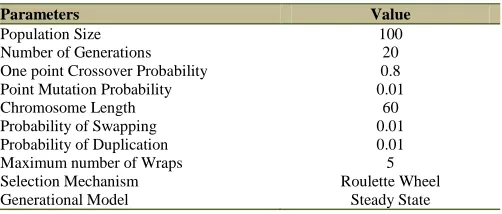
[image:10.612.327.562.364.507.2]In order to find appropriate parameter values for GE-HH, we utilize the Relevance Estimation and Value Calibration method (REVAC) [49]. REVAC is a steady state genetic algorithm that uses entropy theory to determine the parameter values for algorithms. Our aim is not to find the optimal parameter values for each domain, but to find generic values that can be used for both domains. To use the same parameter settings across instances of both domains, we tuned GE-HH for each domain separately and then used the average of them in value obtained by REVAC for all tested instances. In order to have a reasonable trade-off between solution quality and the computational time needed to reach good quality solutions, the execution time for each instance is fixed to 20 seconds. The number of iterations performed by REVAC is fixed at 100 iterations (see [49] for more details). For each domain, the average values over all tested instances for each parameter are recorded. Then, the average values over all parameters are set as the generic values for GE-HH. The parameter settings of GE-HH that have been used for both domains are listed in Table 2.
TABLE 2 GE-HH PARAMETERS
Parameters Value
Population Size 100
Number of Generations 20
One point Crossover Probability 0.8
Point Mutation Probability 0.01
Chromosome Length 60
Probability of Swapping 0.01
Probability of Duplication 0.01
Maximum number of Wraps 5
Selection Mechanism Roulette Wheel
Generational Model Steady State
B. Problem Domain I: Exam Timetabling Problems
Exam timetabling is a well known NP-hard combinatorial optimization problem [50] and is faced by all academic institutions. The exam timetabling problem can be defined as the process of allocating a set of exams into a limited number of timeslots and rooms so as not to violate any hard constraints and to minimize soft constraint violations as much as possible[51]. In this work, we carried out experiments on the most widely used un-capacitated Carter benchmarks (Toronto b type I in [51]) and also on the recently introduced exam timetable dataset from the 2007 International Timetabling Competition, ITC 2007 [15].
1) Test Set I: Carter Uncapacitated Datasets
The Carter datasets have been widely used in the scientific literature[14],[51]. They are un-capacitated exam timetabling problems where room capacities are ignored. The constraints are shown in Table 3.
TABLE 3 CARTER HARD AND SOFT CONSTRAINTS
Symbols Description Hard Constraints
H1Carter: No student can sit more than one exam at the same time.
Soft Constraints
S1Carter: Conflicting exams (with common enrolled students) should be spread as far apart as possible to allow sufficient revision time between exams for students.
The quality of a timetable is measured based on how well the soft constraints have been satisfied. The proximity cost is used to calculate the penalty cost (equation 3) [14].
} 4 , 3 , 2 , 1 , 0 { , / ) ( 1 1 1
i S s w Soft kl m k l i m k carter ... (3) Where: wi=2|4-i| is the cost of scheduling two conflicting exams el and ek (which have common enrolled students) with i timeslots apart, if i=|tl-tk|<5, i.e. w0=16, w1=8, w2=4, w3=2 and w4=1; tl and tk as the timeslot of exam el and ek, respectively.
skl is the number of students taking both exams ek and el, if i=|tl-tk| <5;
m is the number of exams in the problem
S is the number of students in the problems
Table 4 gives the characteristics of the un-capacitated exam timetabling benchmark problem (Toronto b type I in [51]) which comprises 13 real-world derived instances.
TABLE 4 CARTER’S UN-CAPACITATED BENCHMARK EXAM TIMETABLING DATASET
Datasets No. of timeslots No. of exams No. of Students Conflict Density
Car-f-92-I 32 543 18419 0.14
Car-s-91-I 35 682 16925 0.13
Ear-f-83-I 24 190 1125 0.27
Hec-s-92-I 18 81 2823 0.42
Kfu-s-93 20 461 5349 0.06
Lse-f-91 18 381 2726 0.06
Pur-s-93-I 43 2419 30032 0.03
Rye-s-93 23 486 11483 0.07
Sta-f-83-I 13 139 611 0.14
Tre-s-92 23 261 4360 0.18
Uta-s-92-I 35 622 21267 0.13
Ute-s-92 10 184 2750 0.08
Yor-f-83-I 21 181 941 0.29
Note: conflict density = number of conflicts / (number of exams)2
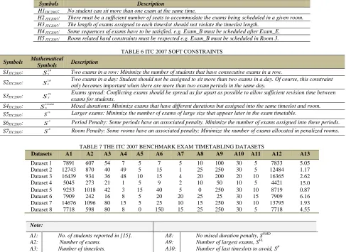
2) Test Set II: ITC 2007 Datasets
The second dataset was introduced in the second International Timetabling Competition, ITC 2007, aiming to facilitate a better understanding of real world timetabling problems and to reduce the gap between research and practice [15]. It is a capacitated problem and has several hard and soft constraints (see Tables 5&6, respectively).
The objective function from [15] is used (see equation 4). The ITC 2007 problem has 8 instances. Table 7shows the main characteristics of these instances.
S
w
S
w
S
w
S
w
S
w
S
w
S
w
R R P p FL FL NMD NMD S s PS S PS D S D R S R ITC Soft
2 2 2 2 22007 ( )
[image:10.612.45.296.370.477.2]TABLE 5 ITC 2007 HARD CONSTRAINTS Symbols Description
H1ITC2007: No student can sit more than one exam at the same time.
H2 ITC2007: There must be a sufficient number of seats to accommodate the exams being scheduled in a given room. H3 ITC2007: The length of exams assigned to each timeslot should not violate the timeslot length.
H4 ITC2007: Some sequences of exams have to be satisfied. e.g. Exam_B must be scheduled after Exam_E. H5 ITC2007: Room related hard constraints must be respected e.g. Exam_B must be scheduled in Room 3.
TABLE 6 ITC 2007 SOFT CONSTRAINTS
Symbols Mathematical Symbols Description
S1ITC2007: S
R S 2
Two exams in a row: Minimize the number of students that have consecutive exams in a row.
S2ITC2007: S
D S
2 Two exams in a day: Student should not be assigned to sit more than two exams in a day. Of course, this constraint only becomes important when there are more than two exam periods in the same day.
S3ITC2007: S
PS S
Exams spread: Conflicting exams should be spread as far apart as possible to allow sufficient revision time between exams for students.
S4ITC2007: S
NMD S 2
Mixed durations: Minimize exams that have different durations but assigned into the same timeslot and room. S5ITC2007: S
FL Larger exams: Minimize the number of exams of large size that appear later in the exam timetable.
S6ITC2007: S
P
Period Penalty: Some periods have an associated penalty. Minimize the number of exams assigned into these periods. S7ITC2007: S
[image:11.612.99.514.264.454.2]R Room Penalty: Some rooms have an associated penalty; Minimize the number of exams allocated in penalized rooms.
TABLE 7 THE ITC 2007 BENCHMARK EXAM TIMETABLING DATASETS
Datasets A1 A2 A3 A4 A5 A6 A7 A8 A9 A10 A11 A12 A13
Dataset 1 7891 607 54 7 5 7 5 10 100 30 5 7833 5.05
Dataset 2 12743 870 40 49 5 15 1 25 250 30 5 12484 1.17
Dataset 3 16439 934 36 48 10 15 4 20 200 20 10 16365 2.62
Dataset 4 5045 273 21 1 5 9 2 10 50 10 5 4421 15.0
Dataset 5 9253 1018 42 3 15 40 5 0 250 30 10 8719 0.87
Dataset 6 7909 242 16 8 5 20 20 25 25 30 15 7909 6.16
Dataset 7 14676 1096 80 15 5 25 10 15 250 30 10 13795 1.93
Dataset 8 7718 598 80 8 0 150 15 25 250 30 5 7718 4.55
Note:
A1: No. of students reported in [15]. A8: No mixed duration penalty, SNMD
A2: Number of exams. A9: Number of largest exams, SFL
A3: Number of timeslots. A10: Number of last timeslots to avoid, SP
A4: Number of rooms. A11: Front load penalty, SR, soft constraints weight[15]
A5: Two in a day penalty, S2D A12: Number of actual students in the datasets.
A6: Two in a row penalty, S2R A13: Conflict density
A7: Timeslots spread penalty, SPS
3) Problem Domain I: Initial Solutions
As mentioned in Section IV-A, GE-HH starts by initializing the adaptive memory mechanism which contains a population of solutions. In this work, we employ hybrid graph coloring heuristics [52] to generate an initial population of feasible solutions for both the Carter and the ITC 2007 instances. The three graph coloring heuristics we utilize are:
Least Saturation Degree First (SD): exams are ordered dynamically, in an ascending order, by the number of remaining timeslots.
Largest Degree First (LD): exams are ordered, in a decreasing order, by the number of conflicts they have with all other exams.
Largest Enrolment First (LE): exams are ordered by the number of students enrolled, in decreasing order. The solution construction method starts with an empty timetable and applies the hybridized heuristics to select and assign the unscheduled exams one by one until all exams have been scheduled. To select an exam, the hybridized heuristic (SD+LD+LE) firstly sorts the unscheduled exams
in a non-decreasing order of the number of available timeslots (SD). Those with equal SD evaluations are then arranged in a non-increasing order of the number of conflicts they have with other exams (LD) and those with equal LD evaluations are then arranged in a non-increasing order of the number of student enrolments (LE). The first exam in the final order is assigned to the timetable. We assign exams to a random timeslot when it has no conflict with those that have already been scheduled (in case of ITC 2007, an exam is assigned to best fit a room), ensuring that all hard constraints are satisfied. If some exams cannot be assigned to any available timeslot, we stop the process and start again. Although there is no guarantee that a feasible solution can be generated, for all the instances used in this work, we were always able to obtain a feasible solution.
4) Problem Domain I: Neighborhood Structures
The neighborhood structures that we employed in the GE-HH framework for both Carter and ITC 2007, which are commonly used in the literature [42], are as follows: Nbe1: Select one exam at random and move it to any feasible
Nbe2: Select two exams at random and swap their timeslots (if feasible).
Nbe3: Select two timeslots at random and swap all their exams. Nbe4: Select three exams at random and exchanges their timeslots at
random (if feasible).
Nbe5: Move the exam causing the highest soft constraint violation to any feasible timeslot.
Nbe6: Select two exams at random and move them to another random feasible timeslots.
Nbe7: Select one exam at random, select a timeslot at random (distinct from the one that was assigned to the selected exam) and then apply the Kempe chain neighborhood operator. Nbe8: Select one exam at random, select a room at random (distinct
from the one that was assigned to the selected exam) and then move the exam to the room (if feasible).
Nbe9: Select two exams at random and swap their rooms (if feasible).
Note that neighborhoods Nbe8 and Nbe9 are applied to ITC 2007 datasets only because they consider rooms. The neighborhood solution is accepted if it does not violate any hard constraints. Thus, the search space of GE-HH is limited to feasible solutions only.
C. Problem Domain II: Capacitated Vehicle Routing
Problems
The capacitated vehicle routing problem (CVRP) is a well-known challenging combinatorial optimization problem [53]. The CVRP can be defined as the process of designing a least cost set of routes to serve a set of customers [53]. In this work, we test GE-HH on two sets of benchmark capacitated vehicle routing problem datasets. These are the 14 instances introduced by Christofides [16] and 20 large scale instances introduced by Golden [17]. The CVRP can be represented as an undirected graph G (V, E), where V= {v0, v1…vn} is a set of vertices which represents a set of fixed locations (customers) and E= {(vi, vj): vi, vj
V, i<j} represents the arc between locations (customers). E is associated with non-negative costs or travel time defined by matrix C= (cij), where cij represents the travel distance between customers vi and vj. Vertex v0represents the depot which is associated with m vehicles of capacity Q1…Qm to start their routes R1…Rm. The remaining vertices v1 … vn represent the set of customers and each customer requestsq1…qn goods and serving time δi. The aim is to find a set of tours that do not violate any hard constraints and minimize the distance. The hard constraints that must be respected are: Each vehicle starts and ends at the depot
The total demand of each route does not exceed the vehicle capacity
Each customer is visited exactly once by exactly one vehicle
The duration of each route does not exceed a global upper bound.
The cost of each route is calculated using (5) [53]:
n
j n
j j i
i c
R C
0 i 1
)
( ……….. (5)
and the cost for one solution is calculated using (6):
m
i i R C f
1
) (
…….. (6)
The two sets of benchmark problems that we have considered in this work have similar constraints and objective function. However, the complexity, instance sizes and customer distributions are different from one set to another.
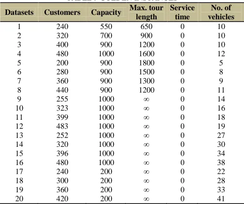
1) Test Set I: Christofides Datasets
[image:12.612.321.569.275.441.2]The first set comprises of 14 instances and was introduced by Christofides [16]. The main characteristics of the problem are summarized in Table 8. The instance size varies from 51 to 200 customers, including the depot. Each instance has a capacity constraint. Instances 6-10, 13 and 14 also have a maximum route length restriction and non-zero service times. The problem instances can be divided into two types: in instances 1-10, the customers are randomly located, whilst, in instances 11-14 the customers are in clusters.
TABLE 8 CHRISTOFIDES INSTANCES
Datasets Customers Capacity Max. tour length
Service time
No. of vehicles
1 51 160 ∞ 0 5
2 76 140 ∞ 0 10
3 101 200 ∞ 0 8
4 151 200 ∞ 0 12
5 200 200 ∞ 0 17
6 51 160 200 10 6
7 76 140 160 10 11
8 101 200 230 10 9
9 151 200 200 10 14
10 200 200 200 10 18
11 121 200 ∞ 0 7
12 101 200 ∞ 0 10
13 121 200 720 50 11
14 101 200 1040 90 11
2) Test Set II: Golden Datasets
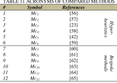
The second CVRP dataset involves 20 large scale instances presented by Golden [17] (see Table 9). The instances have between 200 and 483 customers, including the depot. Instances 1-8 have route length restrictions.
TABLE 9 GOLDEN INSTANCES
Datasets Customers Capacity Max. tour length
Service time
No. of vehicles
1 240 550 650 0 10
2 320 700 900 0 10
3 400 900 1200 0 10
4 480 1000 1600 0 12
5 200 900 1800 0 5
6 280 900 1500 0 8
7 360 900 1300 0 9
8 440 900 1200 0 11
9 255 1000 ∞ 0 14
10 323 1000 ∞ 0 16
11 399 1000 ∞ 0 18
12 483 1000 ∞ 0 19
13 252 1000 ∞ 0 27
14 320 1000 ∞ 0 30
15 396 1000 ∞ 0 34
16 480 1000 ∞ 0 38
17 240 200 ∞ 0 22
18 300 200 ∞ 0 28
19 360 200 ∞ 0 33
[image:12.612.321.568.508.715.2]