The glacial mid depth radiocarbon bulge and its implications for the overturning circulation

The glacial mid-depth radiocarbon bulge and its implications

for the overturning circulation

Andrea Burke1,2, Andrew L. Stewart2,3, Jess F. Adkins2, Raffaele Ferrari4, Malte F. Jansen5,

and Andrew F. Thompson2

1

Department of Earth and Environmental Sciences, University of St. Andrews, St. Andrews, UK,2Division of Geological and Planetary Sciences, California Institute of Technology, Pasadena, California, USA,3_{Department of Atmospheric and Oceanic}

Sciences, UCLA, Los Angeles, California, USA,4Department of Earth, Atmospheric and Planetary Sciences, MIT, Cambridge, Massachusetts, USA,5_{Department of the Geophysical Sciences, University of Chicago, Chicago, Illinois, USA}

Abstract

Published reconstructions of radiocarbon in the Atlantic sector of the Southern Ocean indicate that there is a mid-depth maximum in radiocarbon age during the Last Glacial Maximum (LGM). This is in contrast to the modern ocean where intense mixing between water masses results in a relatively homogenous radiocarbon profile. Ferrari et al. (2014) suggested that the extended Antarctic sea ice cover during the LGM necessitated a shallower boundary between the upper and lower branches of the meridional overturning circulation. This shoaled boundary lay above major topographic features associated with strong diapycnal mixing, isolating dense southern sourced water in the lower branch of the overturning circulation. This isolation would have allowed radiocarbon to decay and thus provides a possible explanation for the mid-depth radiocarbon age bulge. We test this hypothesis using an idealized, 2-D, residual-mean dynamical model of the global overturning circulation. Concentration distributions of a decaying tracer that is advected by the simulated overturning are compared to published radiocarbon data. Wefind that a 600 km (~5° of latitude) increase in sea ice extent shoals the boundary between the upper and lower branches of the overturning circulation at 45°S by 600 m and shoals the depth of North Atlantic Deep Water convection at 50°N by 2500 m. This change in circulation configuration alone decreases the radiocarbon content in the mid-depth South Atlantic at 45°S by 40‰, even without an increase in surface radiocarbon age in the source region of deep waters during the LGM.

1. Introduction

Atmospheric CO2 reconstructed from Antarctic ice cores is highly correlated with Antarctic atmospheric

temperatures, varying between 180 and 290 ppmv from glacial to interglacial periods [Petit et al., 1999;

Siegenthaler, 2005]. The magnitude and pacing of these atmospheric CO2variations over the past 800 kyr

(thousand years) suggest that the ocean plays a key role in driving these changes. In particular, the similar-ity between Antarctic temperature and atmospheric CO2suggests that the mechanisms connecting climate

changes in the Southern Ocean to atmospheric CO2 are likely major drivers of glacial-interglacial CO2

variations [Fischer et al., 2010]. One such hypothesis invokes changes in the strength or position of the westerly winds [Toggweiler et al., 2006;Anderson et al., 2009;Denton et al., 2010], suggesting that a decrease in the strength or an equatorward displacement of the westerlies during the last glacial period would reduce the Ekman transport and upwelling in the Southern Ocean, and thus would reduce the transport of carbon to the surface ocean (and atmosphere) [Toggweiler et al., 2006]. However, ice core evidence sug-gests that there was no significant change in the strength of the westerly winds between the glacial period and today [Fischer et al., 2007], and the evidence to support a latitudinal shift in the westerlies is inconclu-sive [Kohfeld et al., 2013;Sime et al., 2013]. Furthermore, it is necessary to take into account the eddy-driven circulation as well as the wind-driven (Ekman) circulation in order to determine the transport of tracers (such as carbon) in the Southern Ocean. Eddy-resolving models show a much reduced sensitivity of the overturning circulation to changes in wind strength compared to lower resolution models [Munday et al., 2013], indicating that the sensitivity of overturning circulation to changes in the wind might not be as strong as originally thought.

Recent research on the Southern Ocean shows that the combination of eddy and Ekman transport is supported by surface buoyancy forcing [Karsten and Marshall, 2002], and so past variations in surface buoyancy forcing provide an alternative mechanism to alter Southern Ocean circulation (and potentially

Paleoceanography

RESEARCH ARTICLE

10.1002/2015PA002778

Andrea Burke and Andrew L. Stewart contributed equally to this work.

Key Points:

•Greater extent of glacial Antarctic sea ice requires a shoaling of NADW

•Shoaled glacial NADW resulted in more depleted14C at mid-depths

•Isopycnal mixing is important for setting14C distributions in the ocean

Supporting Information:

•Text S1 and Equations (S1)–(S10)

Correspondence to:

A. Burke,

[email protected]

Citation:

Burke, A., A. L. Stewart, J. F. Adkins, R. Ferrari, M. F. Jansen, and A. F. Thompson (2015), The glacial mid-depth radiocarbon bulge and its implications for the over-turning circulation,Paleoceanography,

30, doi:10.1002/2015PA002778.

Received 7 JAN 2015 Accepted 27 MAY 2015

Accepted article online 2 JUN 2015

atmospheric CO2) [Watson and Garabato, 2006].

Furthermore, because the extent of sea ice (which varied by ~5° latitude between the Last Glacial Maximum (LGM; 18–22 ka) and today [Gersonde et al., 2005]) would strongly influence the surface buoyancy forcing in the Southern Ocean, it provides a mechanistic link that ties Antarctic temperature to Southern Ocean circulation and potentially atmospheric CO₂ rise [Fischer et al., 2010]. A recent paper [Ferrari et al., 2014] further extends this connection by linking the extent of glacial sea ice in the Southern Ocean with the depth of North Atlantic Deep Water (NADW) and the boundary between the upper and lower branches of the overturning circulation in the Atlantic, which shoaled to ~2 km in the LGM [Curry and Oppo, 2005;Lund et al., 2011].

Although physical oceanographers rely on surface buoyancyfluxes to place constraints on the rate of deep water formation and overturning circula-tion [Speer and Tziperman, 1992], there is no obvious way to reconstruct past buoyancy fluxes from the sediment record. Instead, paleoceanogra-phers typically use geochemical tracers in the interior of the ocean to reconstruct past circulation [Curry and Oppo, 2005;Lund et al., 2011; Adkins, 2013]. The radiocarbon content of water (as recon-structed from foraminifera or deep-sea corals) is a particularly useful tracer because it provides infor-mation on the amount of time that has elapsed since the water was last at the sea surface. For instance, a comparison (Figure 1) between radio-carbon in the modern Atlantic sector of the Southern Ocean [Key et al., 2004] versus the recon-structed radiocarbon [Barker et al., 2010; Skinner et al., 2010; Burke and Robinson, 2012] from the LGM 8 indicates that the glacial ocean was more isolated from the atmosphere (i.e., the water was

“older” or more depleted in radiocarbon). Additionally, in the LGM profiles there appears to be a “mid-depth age bulge,” where the most radiocarbon-depleted (“oldest”) water is not the deepest water. This feature is mostly absent in the modern Southern Ocean, although there is a slight radiocarbon age bulge in the Pacific sector of the Southern Ocean (Figure 2). The presence of a mid-depth age bulge in the Atlantic sector of the glacial Southern Ocean sug-gests a circulation that differed greatly from the modern.

[image:2.612.174.372.92.359.2]

We combine the insights about surface buoyancy forcing on glacial Southern Ocean circulation [Watson and Garabato, 2006;Fischer et al., 2010] with ocean interior14C reconstructions [Barker et al., 2010;Skinner et al., 2010;Burke and Robinson, 2012] to test the new idea [Ferrari et al., 2014] that the extent of the quasi-permanent sea ice edge around Antarctica plays a crucial role in setting the depth of the boundary between the upper and lower overturning branches and thus the mixing between northern sourced and southern sourced water masses. We hypothesize that the circulation geometry and dynamics that are required by this mechanistic link between the sea ice edge and the boundary between the northern and southern sourced water masses can help to explain the radiocarbon distribution in the glacial high-latitude South Atlantic.

Figure 1.(top) Radiocarbon data plotted as atmosphere normalizedΔ14C (see section 2 for explanation) from the Atlantic sector of the Southern Ocean. Modern water column data are plotted as lines and come from GLODAP [Key et al., 2004]. Measurement uncertainties are smaller than the line width. Data reconstructed from the LGM are plotted as stars

[Burke and Robinson, 2012;Skinner et al., 2010;Barker et al.,

Today, the quasi-permanent sea ice edge approximately coincides with the transition between positive and negative buoyancyfluxes in the Southern Ocean [Ferrari et al., 2014]. South of the sea ice boundary, water becomes denser as a result of cooling and brine rejection. In contrast, north of the sea ice boundary water becomes less dense due to atmospheric warming, precipitation, and melting of transported sea ice and icebergs. These buoyancyfluxes can be used to diagnose the direction of the meridionalflow if the system is in steady state: since surface water increases in density toward the pole, water that is subjected to a negative buoyancy flux flows poleward, and water that is subjected to a positive buoyancyflux flows northward. Thus, water that is upwelled south of the sea ice boundaryflows poleward, forming the lower overturning branch, whereas water that is upwelled north of this boundaryflows equatorward forming the upper overturning branch.

In today’s ocean, the circulation forms one continuous overturning cell [Lumpkin and Speer, 2007;Talley, 2013]. Water sinks in the North Atlantic and is adiabatically upwelled along isopycnals south of the sea ice boundary in the Southern Ocean. It is transformed into Antarctic Bottom Water (AABW) near the continent andflows northward into the Indo-Pacific and Atlantic Basins. In the Atlantic, AABW is mixed with the south-wardflowing North Atlantic Deep Water (NADW) and is thus brought back up to the surface again south of the sea ice edge. In the Indian and Pacific Oceans however, diapycnal diffusion transforms AABW into Indian and Pacific Deep Water (PDW), which is less dense than NADW and thus outcrops farther north in the Antarctic Circumpolar Current. While a fraction of PDW outcrops south of the sea ice boundary and is recycled back into the lower cell as AABW, the remainder outcrops north of the sea ice boundary andflows northward supplying the upper overturning branch, which eventually feeds back into the North Atlantic, thus closing the full overturning circulation. This circulation can be thought of as one continuous overturning loop or a

“figure-eight”circulation.

[image:3.612.216.538.89.275.2]

At the LGM,Ferrari et al. [2014] suggest that a greater equatorward extent of Antarctic sea ice shifted the boundary between negative and positive buoyancy forcing to the north, which resulted in a shoaling of the boundary between the upper and lower overturning circulations in the Atlantic and Indo-Pacific Basins. Shoaling the boundary between these two cells moves it away from the regions of intense mixing near the rough topography of the seafloor [Polzin, 1997;Lund et al., 2011;Adkins, 2013]. The depth of the south-ward PDW return flow to the Southern Ocean was likely similar during the glacial to what it is today (~2000 m) because the depths of the major bathymetric features were the same. Therefore, if the boundary between the upper and lower overturning branches shoals to depths shallower than PDW, then PDW must upwell south of the sea ice edge and so cannot supply the northwardflowing component of the upper cell in the Atlantic [Ferrari et al., 2014]. Instead, the upper cell must close on itself, splitting the LGM overturning circulation into two distinct overturning cells instead of afigure-eight [Ferrari et al., 2014]. We hypothesize that this two-celled circulation is the reason for the pronounced radiocarbon depletion at mid-depths in

the glacial Southern Ocean: not only would radiocarbon-enriched northern sourced waters be limited to the upper ocean, the reduced mixing between northern and southern sourced waters would accentuate the radiocarbon depletion at mid-depth as seen in the modern Pacific [Roussenov et al., 2004].

In this study we test this hypothesis using a two-dimensional residual overturning model with a radioactive tracer. This model setup cannot recreate the modernfigure-eight circulation since it only has one basin, and thefigure-eight circulation requires two distinct basins. However, the model is suitable for testing the impact of expanded sea ice cover in the Southern Ocean on the depth of the boundary between the upper and lower branches of the overturning circulation in the LGM, and allows us to explore the implications of that depth on the radiocarbon distribution in the high-latitude South Atlantic. In section 2 we describe the radiocarbon data compiled from the last glacial period, as well as from modern water column measurements. In section 3 we provide background on the modern theory for the meridional overturning circulation and introduce a two-dimensional model based on that theory. In section 4 we present and discuss results from the model, and we summarize our conclusions in section 5.

2. Radiocarbon Pro

fi

les at the LGM

2.1. Water Column Radiocarbon Data

To highlight the dramatic radiocarbon changes reconstructed for the LGM water column we compare these data to modern profiles near the sample sites. The modern data (both measured and bomb-corrected) for this study were compiled from the Global Data Analysis Project (GLODAP) database [Key et al., 2004]. Measured and bomb-corrected data are plotted in terms ofΔ14C (‰), which is a measure of the relative difference between the radiocarbon activity of an absolute standard and that of the sample, after correcting for both fractionation and the time since the sample was collected. The bomb-corrected data (“naturalΔ14C”) use potential alkalinity to correct the measuredΔ14C for the presence of radiocarbon that can be attributed to nuclear testing and the spike in atmospheric14C.

We plot both individual station data near the locations of sediment cores and corals (Figure 1), as well as regional averages (Figure 2). For the individual stations (Figure 1), we use the measuredΔ14C for deep sam-ples and bomb-correctedΔ14C for shallow and intermediate depths. Although the bomb-correctedΔ14C is an estimate for what the preanthropogenic water column radiocarbon should be, there is unrealistically large and systematic scatter in many bomb-corrected deep samples. Additionally, some deep bomb-corrected14C values are more radiocarbon enriched than what was actually measured, which is the wrong direction of change. In Figure 1, the point at which we switch between measured and bomb-correctedΔ14C is the depth where the two profiles intersect (500 m in the Drake Passage and 1500 m in the South Atlantic). For the regional averages (Figure 2), measured and bomb-corrected radiocarbon data were considered separately, although we only included bomb-corrected data from locations that also had measured radiocarbon (rather than the gridded GLODAPfield). The radiocarbon data from 35–45°S were interpolated to a 200 m depth resolution. Then the data were binned by geographical area (west and east regions of the Atlantic, Pacific, and Indian Oceans), and an average radiocarbon profile was calculated from the interpolated station data within each bin. Error bars represent one standard error of theΔ14C values in each bin.

2.2. LGM Radiocarbon Data

LGM radiocarbon data from the Atlantic sector of the Southern Ocean come from foraminifera from two sedi-ment cores—MD07-3076 (44.1°S, 14.2°W; 3770 m) [Skinner et al., 2010] and TN057-21 (41.1°S, 7.8°E; 4981 m) [Barker et al., 2010]—and a uranium-thorium dated deep-sea coral from the Drake Passage [Burke and Robinson, 2012] (Figure 1, stars). We plot these data as atmosphere-normalizedΔ14C (‰), which is directly com-parable to modern water columnΔ14C (‰) as it takes into account that atmospheric radiocarbon in the LGM was ~40% higher than it is today. In order to calculate this value, it is necessary to have an accurate calendar age for the sample, which is either the uranium-thorium age for the coral or the age model for the sediment core. The calendar age and the radiocarbon age of the sample can then be combined (equation (1)) to determine theΔ14Csample:

Δ14_C sample¼

e

14_{C age} =8033

e Calendar age=8266

1

0 @

1

The two different decay rates (1/8033 years and 1/8266 years) in this equation derive from the initial determination of the radiocarbon half-life (5568 years, known as the Libby half-life [Libby, 1955]), which is still used to convert a measured14C/12C ratio into radiocarbon years, and the more accurate half-life of radio-carbon which was later determined to be 5730 ± 40 years [Godwin, 1962]. After calculatingΔ14C_sample, we nor-malize it with the concurrentΔ14Catm(determined from the IntCal13 atmospheric record [Reimer et al., 2013]) to

get the atmosphere normalizedΔ14C:

Δ14_C

atm normalized¼

Δ14_C samp

1000 þ1

Δ14_C atm

1000 þ1

1

0 @

1

A1000: (2)

For sediment core MD07-3076, there arefive depth intervals within the LGM (18–22 ka) with benthic radiocarbon measurements [Skinner et al., 2010]. For core TN057-21, on the updated age model [Barker and Diz, 2014] there are four depth intervals with benthic radiocarbon measurements within the LGM. In Figure 1 we plot the average and standard deviation of the atmosphere normalizedΔ14C during the LGM at the within of these sediment cores, taking into account uncertainty in the calendar age, radiocarbon measurement, and atmosphericΔ14C record. The shallowest data point (820 m) in Figure 1 comes from a deep-sea coral from the Drake Passage with a U-Th age of 20.27 ± 0.17 kyr B.P. [Burke and Robinson, 2012], and the plotted uncertainty of the atmospheric nor-malizedΔ14C represents one standard deviation based on uncertainty in the U-Th age, the14C measurement, and the atmosphericΔ14C record.

As shown in Figure 1, the Atlantic sector of the glacial Southern Ocean has a radiocarbon depth profile that is characterized by a mid-depth depletion in radiocarbon (maximum in radiocarbon age) or a“mid-depth bulge.”This feature is significantly different from the modern radiocarbon profiles at these sites. A similar feature can be seen in pre-LGM (prior to 25.36 ka [Vandergoes et al., 2013]) radiocarbon data from the Pacific sector of the Southern Ocean; there are large benthic-planktic radiocarbon offsets at mid-depths (2700 m) off the coast of New Zealand [Sikes et al., 2000], although deeper radiocarbon data at this site do not yet exist in the published literature.

2.3. Interpretation

The effect of circulation on radiocarbon in the modern ocean can be seen in depth profiles from the Atlantic and Pacific sectors of the Southern Ocean (Figure 2). In the Pacific sector, there is a hint of a mid-depth radio-carbon bulge resulting from relatively old Pacific Deep Water, which is the returnflow of diffusively upwelled AABW. In contrast, in the Atlantic sector of the Southern Ocean, this mid-depth age bulge is absent due to the presence of relatively radiocarbon-enriched NADW. These two main water masses in the Atlantic differ in radiocarbon content by more than 60‰, and a combination of isopycnal and diapycnal mixing works to homogenize the gradients in radiocarbon content of these waters, as shown in Figure 3.

The approximate boundary between NADW and AABW lies along the neutral density surfaceγn= 28.15 kg/m3 [Jackett and McDougall, 1997;Lumpkin and Speer, 2007]. Tracing the evolution of radiocarbon along neutral density surfaces above and below this boundary provides insight into how mixing in the modern ocean affects the radiocarbon distribution (Figures 3a and 3b). The neutral density surfaceγn= 28.20 kg/m3is within AABW, and the radiocarbon along this surface stays relatively constant until it begins increasing at around 30°S. Because this surface does not outcrop in the northern high latitudes, the source of radiocarbon must be from diapycnal mixing with more radiocarbon-enriched waters above. The deeper neutral density surface

γn

NADW and AABW and is deeper than 3500 m over most of the Atlantic Basin. Although radioactive decay would also decrease radiocarbon content along theflow path of NADW, the rapid decrease in radiocarbon content alongγn= 28.05 kg/m3occurs over a short distance (between 40°S and 60°S), and so radioactive decay is unlikely to be the main cause of this decrease. A plot of salinity versusΔ14C (Figure 3c) from the South Atlantic along neutral density surfaces (γn= 28.12–28.18 kg/m3) shows a simple mixing relation-ship between two end-members (southern and northern); if radioactive decay was important over these spatial scales, then the data would lie on a curved line between the two end-members [Broecker and Peng, 1982;Adkins and Boyle, 1999].

There are two main features of the glacial radiocarbon distribution that stand out when compared to the modern distribution of radiocarbon: (1) overall, the glacial ocean is more radiocarbon depleted than the modern ocean and (2) the maximum radiocarbon depletion is at mid-depths, forming a bulge that is absent in the modern high-latitude South Atlantic Ocean (Figure 1). Previous studies have identified that the glacial ocean was more radiocarbon depleted from the atmosphere than the modern ocean [e.g.,

Skinner and Shackleton, 2004;Robinson et al., 2005;Galbraith et al., 2007;Barker et al., 2010;Skinner et al., 2010;Burke and Robinson, 2012], and this feature has been explained by various processes, including decreased air-sea gas exchange due to increased sea ice cover [Schmittner, 2003] and an increase in the residence time of the deep ocean [Sarnthein et al., 2013]. While these processes would indeed contribute to the greater depletion of radiocarbon, they do not offer a straightforward explanation for the change in the depth structure of radiocarbon in the glacial ocean. Previous studies in the glacial Pacific have shown that there was a stronger gradient in radiocarbon content between surface/intermediate-depth (0–1 km) and mid-depth waters (2.7–3.6 km) during the glacial compared to the modern [Sikes et al., 2000;

a)

[image:6.612.181.573.89.392.2]

b) c)

Galbraith et al., 2007], and this feature also appears to be true in the Atlantic sector of the Southern Ocean [Skinner et al., 2010;Burke and Robinson, 2012] (Figure 1). The added constraints on glacial radiocarbon from the abyssal ocean (~5 km depth [Barker et al., 2010]) imply that the deepest ocean is still relatively well ventilated and that the most radiocarbon-depleted waters (or the oldest waters) lie at mid-depths. In other words, the radiocarbon distribution in the glacial Atlantic looks like a more extreme version of the modern North Pacific.

We suggest that the reconstructed glacial radiocarbon distribution is a consequence of reduced mixing between northern and southern sourced waters in the Atlantic, which results in a more isolated southern sourced water mass. Model studies investigating the response of radiocarbon in the modern North Pacific to changes in the diapycnal mixing show stronger gradients (and a more pronounced“bulge”) when the diapycnal mixing is reduced [Roussenov et al., 2004]. In an earlier companion paper [Ferrari et al., 2014], we put forth the idea that extended Antarctic sea ice during the glacial requires there to be a shoaled boundary between the two overturning branches, and this necessarily confines the northern sourced water mass to the upper overturning branch. Moving this boundary away from rough bottom topography would decrease the diapycnal mixing across the boundary between northern and southern sourced waters [Lund et al., 2011]. The simple lack of northern sourced waters at mid-depths in the high-latitude South Atlantic would result in more depleted radiocarbon at these depths (as evidenced by the difference between the Atlantic and Pacific sectors of the Southern Ocean today (Figure 2)). Additionally, the circulation geometry required by the increased extent of sea ice would force northern sourced waters to upwell north of the sea ice edge forming a separate circulation cell [Ferrari et al., 2014], and thus, the isopycnal mixing between northern and southern sourced waters that is observed in the modern ocean would be reduced. In the following sections, we test these ideas with an idealized two-dimensional model and add a decaying tracer to investigate the effect of shoaling the boundary between the upper and lower circulation branches on the distribution of radiocarbon.

3. Conceptual Model of the Meridional Overturning Circulation

To explain the changes in the radiocarbon depth profiles between the LGM and today we construct a conceptual model of the ocean that includes only the physical elements necessary to test our hypothesized changes in the circulation [Ferrari et al., 2014]. Our model describes the zonal- and time-mean density stratification and overturning circulation in an idealized Antarctic Circumpolar Current (ACC) and northern basin, following Nikurashin and Vallis [Nikurashin and Vallis, 2011]. We allow the model’s overturning circulation to advect a radioactively decaying tracer, and investigate the distribution of this tracer under different patterns of circulation. Our model configuration is sketched in Figure 4. In this section we outline the salient features of our model; full details are provided in the supporting information.

3.1. Tracer Advection and the Role of Mesoscale Eddies

The ocean’s overturning circulation has traditionally been quantified using a streamfunction in latitude-depth space, with mass transport following streamlines. Often incorrectly used for this purpose is the Eulerian mean streamfunction, defined as

ψmeanðy;zÞ ¼

∫

0

zv yð ;z′Þ dz′; (3)

wherevis the meridional velocity, and for simplicity, we assign Cartesianyandzcoordinates to latitude and depth, respectively. At each depthψ_meanmeasures the northward transport between that depth and the surface by the mean velocity; the overbar indicates an average in time and longitude. However,ψ_meanis not actually the streamfunction that transports tracers [e.g., Döös and Webb, 1994]: an additional component due to eddies,ψ_eddy, must be added to account for the transport of mass by mesoscale eddies [McIntosh and McDougall, 1996;Karsten and Marshall, 2002],

ψtrc¼ψmeanþψeddy; ψeddy≈

v′γ′ γz :

(4)

addition to advection by the meanflow. Here

γdenotes neutral density, and primes denote departures from the time/longitudinal aver-age, i.e.,γ¼γþγ′. We denote the overturning streamfunction as ψtrc to emphasize that it

describes the paths of tracer particles in the absence of other effects, such as mixing. In the oceanographic literature, ψtrc is also

referred to as the “residual” streamfunction

ψres, or simply asψ.

In practice, the difference betweenψ_meanand

ψtrc is most obvious in the ACC, where the

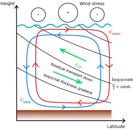
strong westerly winds drive a mean northward Ekman transport within the surface mixed layer. There are no lateral boundaries in the upper ocean across the latitudes spanning the ACC, so the mean streamfunctionψmean

is closed by a southward returnflow beneath the Drake Passage sill depth (~2 km) [Zika et al., 2013]. The tilted isopycnals in the ACC are baroclinically unstable, sustaining a vigorous mesoscale eddy field that releases potential energy by relaxing the isopycnal slopes. The resulting transport of mass via the eddy streamfunction ψeddy almost

com-pletely compensatesψmean, leavingψtrc as a

[image:8.612.177.572.88.315.2]

relatively small residual that tends to be aligned with the isopycnals [Marshall and Radko, 2003]. These concepts are illustrated schematically in Figure 5.

Figure 4.Schematic of our conceptual model of the MOC, corresponding to our Atlantic-like modern reference case. The thick arrows indicate mass transports, and thin curvy arrows indicate the directions of buoyancyfluxes. The green and yellow arrows correspond to lower and upper overturning cells, respectively. In the model,Lbasin≫Lchannel(the schematic is not to scale).

Figure 5.Schematic of the residual overturning circulation in the ACC. Strong westerly winds drive a northward Ekman transport at the ocean surface, with a returnflow at the ocean bed (the“mean” circulation, red arrows). This shoals the density surfaces (isopycnals, black curves) to the south. The energy stored in the tilted isopycnals is released via the generation of mesoscale eddies, untilting the isopycnals in the process. This movement of water associated with this untilting is referred to as the eddy circulation (blue arrows). The mean and eddy circulations oppose each other but have a nonzero sum (the“tracer”or residual circulation,ψtrc,

[image:8.612.173.386.375.585.2]

3.2. Residual-Mean Conceptual Model of the Meridional Overturning Circulation

Our residual-mean model solves for the mean neutral density γ and tracer streamfunction ψtrc

in an idealized ACC/Southern Ocean channel (70°

S45°S) connected to an extended northern basin (45°S–50°N), as shown in Figure 4. For simpli-city the longitudinal extent of the domain is taken to be a constant, L_x= 28,000 km, approximately equal to the Earth’s circumference at 45°S. In the Southern Ocean, above the topographic sill at

Zsill=2 km, the mean and eddy components

of ψtrc are related to the surface wind forcing

and stratification via

ψmean¼

τ ρ0f

;ψeddy¼Ks;

for 70°S<y<45°S; z >2000 m: (5)

The mean componentψ_meanmay be derived by vertically integrating the zonal momentum budget from the ocean surface [Marshall and Radko, 2003], and states that all mean northward transport is con-tained in the wind-driven surface Ekman layer. Hereτis the zonal surface wind stress,ρ0= 1000 kg m3is the

reference density,s¼ γ_y=γ_zis the mean isopycnal slope, andf=104s1is the Coriolis parameter. To sim-plify the interpretation of our model results, we set these parameters as uniform constants. The eddy compo-nentψeddyemploys a Gent and McWilliams [Gent and Mcwilliams, 1990] downgradient parameterization of the

meridional eddy densityflux with diffusivityK, and thereby becomes proportional to the mean isopycnal slope

s. In the northern basin the isopycnals are assumed to beflat, and the vertical transport is determined by the change inψ_trcbetween the northern and southern ends of the basin [Nikurashin and Vallis, 2011]. Below the sill depth, the mean streamfunctionψmeanis reduced linearly to zero at the ocean bed, which serves as a simple

representation of the mean southward geostrophic returnflow in the Southern Ocean [Ito and Marshall, 2008]. The buoyancy diffusivityKis also reduced linearly to zero over the same range of depths in order to avoid creating a singularity at the ocean bed.

Asfluid parcels are advected, they are subject to small-scale diapycnal mixing due to internal wave break-ing, parameterized via a diffusivity κ_dia. In our model, the diapycnal diffusivity varies (Figure 6) from

κsurf= 105m2s1 at the surface toκdeep= 104m2s1in the deep ocean, with a rapid transition across

the sill depthZ_sill,

κdia¼

1

2 κsurfþκdeep

þ1₂ κsurfκdeep

tanh zZsill

Hsill

: (6)

This idealized profile reflects the intensification of diapycnal mixing close to rough bathymetry and was designed to capture the transition between large vertical values at the ocean bottom and small values at depths above the top of most ridges and rises. The top and bottom values are representative values based from oceanic estimates [Nikurashin and Ferrari, 2013;Waterhouse et al., 2014]. HereHsill= 750 m measures

the vertical extent of the transition between the weakly mixed surface and the strongly mixed abyss.

Ferrari et al. [2014] hypothesize that this transition is key to the shoaling of NADW with the expansion of Southern Ocean sea ice at the LGM.

In the Southern Ocean, thermodynamic surface fluxes beneath ice are crudely parameterized as a prescribed uniform density input Γice= 1.5 × 107kg m2s1 over a latitudinal extentLice from the

[image:9.612.199.341.92.296.2]

southern boundary. In the “modern” model ocean (L_ice= 500 km), the total density input beneath Antarctic ice compares closely with the Southern Ocean State Estimate [Mazloff et al., 2010]. North of this,

Figure 6.Diapycnal diffusivity profile used in our 2-D model. The increase with depth reflects the enhanced diapycnal diffusivities found close to major bathymetric features, which extend to around 2000 m depth in the Atlantic and Pacific

we apply a buoyancyflux that restores the density in the surface model grid boxes to a prescribed linear profile over a time scale ofT_γ= 2 weeks, ranging fromγ¼27:9 kg m3_{at the ice edge toγ¼25:9 kg m}3_at

45°S. This reflects the rapid equilibration of ocean surface temperature with the atmosphere [Haney, 1971] and the general warming toward the equator.Ferrari et al. [2014] identifyγ¼27:9 kg m3_{as the isopycnal that}

emanates from the quasi-permanent sea ice edge at the ocean surface and separates the upper and lower branches of the present-day global meridional overturning circulation (MOC).

Our residual-mean model cannot directly simulate the process of deep convection, so at the southernmost and northernmost edges of our model domain, we add convective regions of widthLAABW= 100 km and

LNADW= 150 km, respectively. In these regions we assume that convective motions vertically homogenize

density and linearly map deep isopycnals to the ocean surface, as shown in Figure 4 and explained in the supporting information. In the AABW convective region the surface density input is afixedflux with an exponential profile, but the average density input remains equal to Γice, defined above. The NADW

convective region parameterizes formation of NADW within the deep North Atlantic marginal seas [Spall, 2004, 2011]. The density input takes the form of a relaxation toward a prescribed density

γNADW= 28.1 kg m3, which corresponds approximately to the density of Denmark Strait Overflow Water,

with a time scaleT_NADW= 10 years.

Once our model ocean has established a steady density distribution and tracer streamfunction, we solve for the mean distribution of radiocarbon, which we denote as C for convenience. Radiocarbon is similarly advected byψ_trcand diffused across isopycnal surfaces byκ_dia, in addition to decaying with a half-life of 5730 years. Importantly, radiocarbon, as a dynamically passive tracer, is stirredalongisopycnal surface by mesoscale eddies, an effect that we parameterize using a uniform constant isopycnal diffusivity

κiso. We impose a surfaceflux of radiocarbon that restores the concentration in the model surface grid

boxes, with a time scale ofT_c= 1 year, to a constant value of125‰beneath ice in the Southern Ocean, a constant value of50‰at 45°S and throughout the northern basin, and linearly varying between the two. This profile qualitatively captures the structure of modern surface ocean radiocarbon reconstructions [Bard, 1988;Key et al., 2004]. Radiocarbon is similarly restored to its surface concentration in the high-latitude convection regions, under the assumption that it is mixed rapidly throughout the water column by deep convection. We emphasize here that our goal is not to predict the surface radiocarbon distribution. Rather, we will investigate how the deep radiocarbon distribution is modified by changes in the ocean circulation, treating the modern radiocarbon distribution as a surface boundary condition.

We have purposefully made the simplest choices possible for the various model parameters described above. We have therefore constructed a model of minimal complexity, including only the most salient features of the ocean circulation. To summarize, these features are (1) residual mean overturning circulation in the channel, (2) convection at the northern and southern boundaries of the model domain, (3) stratification in the basin that is set at the northern edge of the channel, and (4) a southward returnflow below the depth of the sill in the channel. Consequently, the model output should not be expected to compare precisely with the real ocean; rather, it illustrates the qualitative response of large-scale features of the ocean circulation and radiocarbon distribution to changes in surface forcing.

and Samuels, 1993]. Although diffusive upwelling of deep waters across the thermocline is missing in our model, they represent a relatively small transport compared to the returnflow of PDW to the Southern Ocean surface. Thus, our model is well posed to assess whether increased sea ice extent in the Southern Ocean would shoal the boundary between the upper and lower overturning branches and the influence of the depth of this boundary on the distribution of radiocarbon in the glacial ocean.

4. Model Results

4.1. The Modern Ocean

We define a reference (or modern) case in which the sea ice extent isLice= 500 km, the surface wind stress is

τ= 0.1 N m2, and the buoyancy diffusivity and isopycnal diffusivity areK=κiso= 1000 m2 s1. This leaves

around 2000 km of the channel surface ice-free and yields an estimate for the ACC isopycnal slope of

s≈103, so that theγ¼27:9 kg m3_{isopycnal lies close to 2000 m depth in the basin region, in agreement}

[image:11.612.216.531.86.480.2]

with observations [Ferrari et al., 2014]. This configuration is Atlantic- like in the sense that there is a deepwater source at the northern boundary. For comparison, we also define a Pacific-like reference case

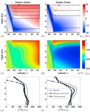
(Figures 7b, 7d, and 7f) with identical parameters, but we remove northern deep water formation by turning off surface restoring in the northern convection region.

Figures 7a and 7b compare the density stratification and overturning streamfunction between our Atlantic-like and Pacific-like reference simulations. In both of these reference simulations, water is exported at all depths from the AABW convective region and enters the northern basin below 4000 m. It then upwells diffu-sively across density classes and returns southward along isopycnals to the surface, where it becomes denser due to density input under sea ice, and thusflows southward. In our Pacific-like simulation, the upper over-turning cell is weak, and northern sourced water sinks to a depth of 1500 m. In our Atlantic-like simulation, the upper overturning cell is much stronger: NADW is exported down to 4000 m from the northern convec-tive region and upwells to around 2000 m as itflows southward. It then upwells along isopycnals to the sur-face of the Southern Ocean, where the sursur-face restoring increases its buoyancy and drives the waters northward. Notice again that the model here is idealized in that it represents the overturning in the two basins as independent. In the real ocean the circulations in the two basins are connected as discussed in section 1.

Figures 7c and 7d show that the presence of North Atlantic deep convection dramatically alters the radiocarbon distribution in the deep ocean. In our Pacific-like simulation the absence of northern deep convection results in water withΔ14C =230‰in the mid-depth northern basin. By contrast, in the Atlantic-like simulation the most radiocarbon-depleted waters haveΔ14C =160‰ and lie at mid-depth close to 45°S. Figures 7e and 7f compare the simulated radiocarbon profiles at 45°S with radiocarbon profiles from the western Atlantic and eastern Pacific (see Figure 2). Below 1500 m, Atlantic radiocarbon is relatively uniform, withΔ14C between 135‰ and 160‰, while the Pacific exhibits a mid-depth bulge ofΔ14C =220‰at 2400 m. Our idealized Atlantic-like and Pacific-like simulations capture the qualitative features of the actual profiles.

Even in our idealized two-dimensional circulation model, several physical processes contribute to the distribution of radiocarbon (see supporting information). In order to identify which processes are most important for radiocarbon as a tracer, we conducted a series of model runs with the same circulation and stratification, but when calculating the radiocarbon distribution we independently activated or deac-tivated the residual circulationψtrc, isopycnal mixingκiso, and diapycnal mixingκdia. Figure 8 shows the

radiocarbon profiles at 45°S for each parameter combination in our Atlantic-like (Figure 8a) and Pacific-like (Figure 8b) simulations. In the simulation with only diapycnal mixing enabled, bottom waters haveΔ14C values of730‰, due to the slow time scale associated with vertical diffusion. Including the residual circulation dramatically improves the profiles, but aΔ14C =260‰(Atlantic) orΔ14C =300‰(Pacific) mid-depth bulge remains due to the long transit time for AABW to travel from the southern boundary to

[image:12.612.203.546.92.230.2]

(a) (b)

Figure 8.Radiocarbon profiles in our (a) Atlantic-like and (b) Pacific-like modern reference simulations, in which changes in radiocarbon due to the overturning circulationψtrc, isopycnal mixingκiso, and diapycnal mixingκdiahave been independently

the northern boundary and then return to 45°S. The Atlantic case has a less pronounced mid-depth bulge because of the presence of northern sourced waters at mid-depths; however, it maintains a bulge because the water at mid-depths has a longer transit time from its source region than the waters above and below. The addition of isopycnal mixing reveals two surprising features: (i) isopycnal mixing is necessary to obtain a mid-depth radiocarbon content that lies even remotely close to observations and (ii) isopycnal mixing

alonecan produce a mid-depth bulge in the Pacific, but not in the Atlantic, as in the modern ocean.

To understand feature (i) physically, we use the radiocarbon evolution equation (equation (S10) in the supporting information) to create a straightforward estimate of the time scales over which advection, isopycnal mixing, diapycnal mixing, and radioactive decay affect the radiocarbon concentration at 45°S,

Tadv¼

HLbasin

ψtrc

½ ; Tiso¼

L2_channel κiso ;

Tdia¼

H2 κdia ;

Tdecay¼

1

r : (7)

These are derived by comparing each term in equation (S10) to the time derivativeCt, and replacing partial

derivatives with simple scalings, e.g.,Cz∼C0/Hor∂ψtrc/∂y∼[ψtrc]/Lchannel, where [ψtrc] is an estimate of the

strength of the overturning streamfunction andC0is a typical radiocarbon concentration. For example, for

diapycnal mixing we take Ct∼ κdiaCz

z, so C0/Tdia∼κdiaC0/H2, and therefore, we choose Tdia=H2/κdia.

Importantly, we useLchannelas the length scale for isopycnal mixing, rather thanLbasin: radiocarbon mixed

isopycnally to mid-depth at 45°S is sourced either from the surface of the Southern Ocean or from the northern convection region. The Southern Ocean surface is much closer (∼Lchannel) and therefore

supplies radiocarbon much more rapidly to 45°S. By contrast,Lbasinis the correct horizontal length scale

for advection becausefluid parcels advected to mid-depth at 45°S must typically traverse the length of the northern basin, following the streamlines shown in Figure 7. SubstitutingH= 5000 m,Lbasin= 10, 000 km,

Lchannel= 2500 km,κiso= 1000 m2s1,κdia= 104m2s1, and [ψtrc] = 0.5 m2s1into equation (7) yields

estimates ofT_adv≈3.2 kyr,T_iso≈0.2 kyr,T_dia≈7.9 kyr, andT_decay≈8.3 kyr. Thus, the time scale for isopycnal mixing is more than an order of magnitude shorter than any other process, and so the relatively high radiocarbon content of the water column at 45°S is principally due to isopycnal mixing.

To understand feature (ii),first note that in Figures 7a and 7b, small variations in the isopycnal slope result in substantial“thickness gradients,”where the vertical spacing between isopycnals changes with latitude. As indicated in Figure 5, these thickness gradients are necessary to support the latitudinal advective transport across the ACC, and therefore to close the overturning cells. However, they have additional implications for isopycnal mixing: where waters upwell from mid-depth in the Pacific to the surface of the Southern Ocean, the isopycnal thickness decreases southward. These density classes therefore outcrop over a relatively narrow surface area and receive a relatively smallflux of radiocarbon from the atmosphere. Thus, isopycnal mixing is less effective at maintaining the radiocarbon content of the mid-depth waters than the near-surface or abyssal waters.

We emphasize that the surprisingly strong influence of isopycnal mixing should not be interpreted to mean that the overturning circulation is unimportant for the radiocarbon content at 45°S. If there were no overturning circulation then no isopycnal thickness gradient would exist in the ACC, and so isopycnal diffusion could no longer produce a mid-depth bulge. Furthermore, Figure 8b shows that the structure of the mid-depth bulge is substantially shaped by the overturning circulation and diapycnal mixing, rather than isopycnal mixing alone.

4.2. Sea Ice Expansion and the Transition From Modern to LGM

Ferrari et al. [2014] analyzed Community Climate System Model version 3 (CCSM3) simulations of the modern and LGM climates [Otto Bliesner et al., 2007], which suggest that the quasi-permanent Antarctic sea ice extended around 5° further north at the LGM. Reconstructions of sea ice extent based upon diatom and radiolarian assemblages from LGM sediment also indicate an increased extent of both summer and winter sea ice [Gersonde et al., 2005]. We therefore define an LGM reference experiment in which the sea ice extends by 600 km, settingLice= 1100 km and keeping all other parameters identical to our modern

[image:14.612.176.374.87.534.2]

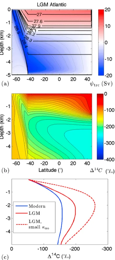
Figure 9a shows the stratification and overturning circulation for our LGM reference simulation. Neutral density is not defined for the LGM, so we have retainedγ¼27:9 kg m3_{as the surface}

density at the sea ice edge for the purpose of comparison (we are free to make this choice because adding a constant to γ everywhere in the domain does not change the solution). The expansion of the sea ice shoals this isopycnal by around 600 m and with it the deep cell of the MOC. As a result, NADW no longer sinks below 2000 m, and thus, it is subject to much weaker diapycnal diffusivity, resulting in a largely adiabatic southwardflow along isopycnals to the surface of the Southern Ocean.

Figure 9b shows that shoaling the NADW above 2000 m ages the waters at the deep northern boundary, producing a radiocarbon distribution that more closely resembles the Pacific-like mod-ern reference simulation. This result is supported by available reconstructions of older (more radio-carbon depleted) water in the deep North Atlantic during the LGM [Keigwin, 2004; Robinson et al., 2005;Skinner et al., 2014]. Shoaling NADW above 2000 m removes the source of radiocarbon-rich water in the mid-depth northern basin, so the

Δ14_{C of mid-depth waters at 45°S decreases by}

~40‰, as shown in Figure 9c. As discussed above, isopycnal mixing also plays a key role in moderat-ing the magnitude of the mid-depth radiocarbon bulge at 45°S, and so the oldest curve in Figure 9c corresponds to an extreme case in which the sea ice is extended toLice= 1100 km and the isopycnal

diffusivity is reduced toκiso= 100 m2s1.

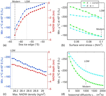
To illustrate the importance of the circulation’s interaction with the vertical mixing profile we have conducted simulations for sea ice extents ranging fromL_ice= 500 km toL_ice= 2000 km, as shown in Figure 10a. As the sea ice expands, the radiocarbon content of mid-depth waters decreases rapidly due to the shoaling of NADW. The NADW shoals most rapidly betweenLice= 500 km andLice= 1100 km

because over this range, theγ¼27:9 kg m3_{isopycnal shoals from the sill depth of 2000 m up to around}

1400 m and the diapycnal diffusivity on that isopycnal decreases from κdia= 105 m2s1 to

κdia≈1 × 105 m2s1 (Figure 6). Recall that γ¼27:9 kg m3 marks the sea ice edge, and thus the

division between the upper and lower overturning cells at the ocean surface. Any NADW that sinks deeper than

γ¼27:9 kg m3_{at the northern boundary must upwell across this isopycnal before reaching the surface in}

the Southern Ocean. In the modern case, strong diapycnal mixing permits a large fraction of the NADW to sink to 4000 m and then upwell acrossγ¼27:9 kg m3_{. At the LGM, weak diapycnal mixing shallower in the water}

column essentially confines NADW to lie shallower thanγ¼27:9 kg m3_{, with the same northern boundary}

conditions as in our modern simulations. This is consistent with theFerrari et al. [2014] hypothesis that NADW can only sink below the sill depth as long as theγ¼27:9 kg m3_{isopycnal also lies below the sill.}

To demonstrate that the shoaling of NADW with increasing sea ice extent is a robust feature of this model, we have conducted a series of simulations with LGM sea ice cover (Lice= 1100 km) and NADW density increasing

fromγ_NADW= 28.1 kg m3toγ_NADW= 29.1 kg m3. The largest densities in our modern and LGM reference simulations were close to 28.2 kg m3and 28.5 kg m3, respectively, so this constitutes an extreme range of NADW densities. Figure 10c shows that increasingγNADWsomewhat offsets the shoaling effect of the

sea ice expansion, but bringing NADW as deep as 3000 m requires an extreme increase in density to

γNADW= 29.1 kg m3. In this case the very large density input in the northern convective region produces a

strong stratification in the deep ocean that allows NADW to upwell acrossγ¼27:9 kg m3_{, despite very weak}

diapycnal mixing on that isopycnal. Finally, although the overturning circulation is sensitive to the diffusivity profile (Figure 6) employed in the model [Nikurashin and Vallis, 2011, 2012], the expansion of sea ice results in significant shoaling of NADW at the northern boundary for pretty much any sensible mixing profile which decreases rapidly above major topographic ridges. This is because with a sea ice expansion, the only isopycnals that connect to the portion of the surface that gains buoyancy from the atmosphere are sitting above ridges and rough bathymetry, where the diffusivity is weak. As long as topography and the associated mixing profile are not changed between our modern and LGM scenarios, we are led to conclude that this connection between sea ice extent and NADW depth is robust to the shape of the diffusivity profile.

(a)

(c)

(b)

[image:15.612.187.560.90.430.2]

(d)

Figure 10.(a)Δ14C of the mid-depth bulge at 45°S and maximum depth of NADW formation from a series of model runs with increasing sea ice extent in the Southern Ocean. The modern Atlantic-like and LGM reference cases are indicated. (b)

Δ14_{C of the mid-depth bulge at 45°S over a range of surface wind stress magnitudes, using either the modern or the}

A common hypothesis used to explain differences in the deep ocean circulation during the glacial period relies on shifts in the location and strength of the Southern Hemisphere westerly winds [Toggweiler et al., 2006;Anderson et al., 2009]. We explore how this mechanism would affect the radiocarbon distribution by conducting a series of simulations with surface wind stresses ranging fromτ= 0.05 Nm2toτ= 0.1 Nm2, using both modern and LGM sea ice extents, as well as with and without eddy saturation. The eddy saturation hypothesis argues that the buoyancy diffusivityKin the ACC adjusts linearly with the surface wind stress, such that the isopycnal slope in the Southern Ocean remains unchanged [Munday et al., 2013]. Wefind that reducing the surface wind stress alone reduces the isopycnal slope in the channel and thereby shoals the γ¼27:9 kg m3 _{isopycnal that separates the upper and lower overturning cells. This shoaling}

results in older radiocarbon ages at mid-depth (Figure 10c). This effect is offset when eddy saturation is included, particularly at the LGM. Furthermore, a 50% reduction in the wind stress is required to reduce radiocarbon in mid-depth waters at 45°S by 20‰, in contrast to the 40‰reduction associated with a greater sea ice extent. This 50% reduction in the wind stress is far greater than the most recent estimates from paleoarchives, which suggest at most a 10% change in the westerly wind stress at the LGM [Fischer et al., 2007, 2010;Kohfeld et al., 2013;Sime et al., 2013].

In our reference experiments we simply setκisoequal to the buoyancy diffusivityK, which in turn was selected

to produce a realistic isopycnal slope in the Southern Ocean, but in reality, these diffusivities may differ substantially [Abernathey and Marshall, 2013]. The isopycnal diffusivity is one of the least well-constrained parameters in our model, although our reference value ofκiso= 1000 m2s1lies just within the error range

of the ACC isopycnal diffusivity measured in the Diapycnal and Isopycnal Mixing Experiment in the Southern Ocean (DIMES) [Tulloch et al., 2014]. There are currently no observational constraints for the isopycnal diffusivity in the northern basins; it may vary substantially between the surface-intensified gyre circulations and the deepflows of NADW and AABW. We investigate the model sensitivity toκisovia an

additional series of radiocarbon-only simulations using the reference circulation and stratification but with isopycnal diffusivities ranging fromκiso= 0 toκiso= 2000 m2s1. Figure 10d shows that radiocarbon in the

modern and LGM simulations are strongly sensitive toκ_iso: halvingκ_isomay decrease mid-depth radiocarbon at 45°S by ~30‰. However, aκisoof 100 m2/s is likely not physical.

5. Discussion and Conclusions

In this article we have demonstrated that the high-latitude South Atlantic during the LGM has a pronounced mid-depth bulge in radiocarbon, and this feature is consistent with a shoaling of northern sourced waters and expansion of southern sourced waters. The mid-depth waters (at 3.7 km) are 150‰more depleted than the waters at 1 km and 100‰more depleted than the abyssal waters (5 km). By contrast, the mid-depth bulge in the modern South Pacific is only 40‰ more depleted than the abyssal waters and 120‰ older than the waters at 1 km, and the age maximum lies around 2–3 km. Our idealized model results consistently predict an age maximum around 2–3 km. There are currently no LGM radiocarbon reconstructions from this depth range in the high-latitude South Atlantic, so the available data may underestimate the size of LGM mid-depth bulge.

The aging of the mid-depth South Atlantic is an expected consequence of the reorganization of the overturning circulation at the LGM, as discussed in our companion paper [Ferrari et al., 2014]. The expansion of the Antarctic sea ice at the LGM [Gersonde et al., 2005] shifts equatorward the transition from negative to positive surface buoyancyfluxes in the Southern Ocean [Fischer et al., 2010], and thus the division between southwardflowing and northwardflowing surface waters. This in turn raises theγ¼27:9 kg m3isopycnal, which separates the branches of the overturning circulation in the Southern Ocean, above the topographic sill depth (~2 km). This precludes any southern sourced waters from upwelling aboveγ¼27:9 kg m3_{and being}

To test this hypothesis we constructed an idealized two-dimensional residual-mean circulation model with a rapid increase in diapycnal mixing below 2 km depth, and imposed an expansion of the sea ice around Antarctica (compare Figures 7a and 9a). Expanding the sea ice by 600 km (~5°) raises theγ¼27:9 kg m3

isopycnal by around 600 m, and thereby shoals the depth of NADW formation by around 2500 m (Figure 10a). As argued byFerrari et al. [2014], NADW formed beneath the depth of most ridges cannot upwell diffusively across the shoaledγ¼27:9 kg m3_{isopycnal at the LGM, so the deep ocean responds}

by becoming increasingly dense until NADW sinks to above the ridge depth. Consequently, increasing the density of newly formed NADW has little impact on the depth to which it sinks (Figure 10c). The shoaling of NADW dramatically reduces lateral mixing between northern and southern sourced waters, as the upper and lower overturning cells no longer share isopycnals (contrast Figures 7a and 9a). Via this mechanism the sea ice expansion alone decreases radiocarbon content in the mid-depth waters by ~40‰, making them ~45‰more depleted than the deepest waters and ~50‰more depleted than the waters at 1 km depth (Figure 9c).

This glacial shoaling of NADW is consistent with other LGM proxy records, including glacial reconstructions of water mass distributions from conservative tracers (δ18O) and nutrient proxies (e.g.,δ13C and Cd/Ca) [Curry and Oppo, 2005;Marchitto and Broecker, 2006;Lund et al., 2011]. A recent study [Gebbie, 2014] put forth the suggestion that the available LGMδ18O,δ13C, and Cd/Ca data in the Atlantic can be explained by a slowing of the upper overturning circulation without any significant shoaling. However, this result is obtained without imposing that the glacial circulation in the global ocean is dynamically consistent. Specifically, our model circulation satisfies momentum and buoyancy equations for a given surface forcing (winds and buoyancy fluxes) and interior properties (diapycnal diffusivity). We are unable to recover a slower, deep overturning without a dramatic (arguably unrealistic) alteration of the Southern Ocean buoyancyfluxes, deep diffusivity, or NADW production. Furthermore, Nikurashin and Vallis[2012] and

Kostov et al. [2014] have shown that a slower overturning cell is by necessity shallower. In our model the reduced radiocarbon content is a result of a change in the overturning cell structure as opposed to the strength of that overturning.

Our model suggests that the absence of the mid-depth radiocarbon bulge in the modern South Atlantic is principally due to the presence of northern sourced waters at mid-depths and isopycnal mixing by mesoscale eddies (Figure 8). If true, this means that deep radiocarbon profiles may be used to infer the volumes of the southern and northern sourced waters but tell us little about the strength of the circulation. The effects of isopycnal diffusion may be particularly pronounced in radiocarbon because radioactive decay leads to the formation of strong isopycnal gradients, absent in conservative tracers likeδ18O.

The model employed in this study is highly idealized, incorporating the simplest possible parameter choices to obtain a qualitatively correct representation of the overturning circulation. This allows the mechanisms controlling both modern and LGM radiocarbon ages to be readily understood. Yet there are some important caveats to this approach. Being two-dimensional, our model is unable to represent the“figure-of-eight” structure of the modern overturning circulation, which would require separate representations of the Atlantic and Pacific Basins. Nevertheless, the model captures the key mechanism underlying the formation of the mid-depth bulge at the LGM: shoaling of NADW concurrent with the expansion of Antarctic sea ice, resulting in reduced mixing between northern sourced and southern sourced waters. However, the use of what is essentially a single, global northern basin may underestimate the relative importance of advection in setting radiocarbon distributions. If the modeled modern southward transport of northern sourced waters was instead concentrated in boundary currents in a narrow Atlantic Basin, the velocities associated with thatflow would be larger and might further reduce the radiocarbon age of the mid-depth South Atlantic via advection of radiocarbon-enriched waters from the North Atlantic surface. This could account for the slight, oppositely signed, mid-depth bulge in radiocarbon age in the modern South Atlantic (Figure 2).

LGM could increase the surface reservoir age beneath sea ice (beyond which would be expected from simply air-sea gas exchange limitation), and thereby further increase the age of the mid-depth bulge. Additionally, the core data plotted in Figure 1 were retrieved from sites spanning ~70° of longitude and ~20° of latitude, and the sparseness of paleoceanographic data in the region precludes quantification of how accurately these samples represent the broader South Atlantic. Both more radiocarbon reconstructions of the glacial ocean and a three-dimensional treatment of ocean circulation will help to ultimately resolve this discrepancy, and would yield further insight into the transition between the modern and LGM overturning circulations.

References

Abernathey, R. P., and J. Marshall (2013), Global surface eddy diffusivities derived from satellite altimetry,J. Geophys. Res. Oceans,118, 901–916, doi:10.1002/jgrc.20066.

Adkins, J., and E. A. Boyle (1999), Age screening of deep-sea corals and the record of deep North Atlantic circulation change at 15.4 ka, inReconstructing Ocean History: A Window Into the Future, edited by F. Abrantes and A. Mix, pp. 103–120, Plenum, New York. Adkins, J. F. (2013), The role of deep ocean circulation in setting glacial climates,Paleoceanography,28, 539–561, doi:10.1002/palo.20046. Anderson, R. F., S. Ali, L. I. Bradtmiller, S. H. H. Nielsen, M. Q. Fleisher, B. E. Anderson, and L. H. Burckle (2009), Wind-driven upwelling in the

Southern Ocean and the deglacial rise in atmospheric CO2,Science,323(5920), 1443–1448, doi:10.1126/science.1167441.

Bard, E. (1988), Correction of accelerator mass spectrometry14C ages measured in planktonic foraminifera: Paleoceanographic implications,

Paleoceanography,3(6), 635–645, doi:10.1029/PA003i006p00635.

Barker, S., and P. Diz (2014), Timing of the descent into the last Ice Age determined by the bipolar seesaw,Paleoceanography,29, 489–507, doi:10.1002/2014PA002623.

Barker, S., G. Knorr, M. J. Vautravers, P. Diz, and L. C. Skinner (2010), Extreme deepening of the Atlantic overturning circulation during deglaciation,Nat. Geosci.,3(8), 567–571, doi:10.1038/ngeo921.

Broecker, W. S., and T. H. Peng (1982),Tracers In The Sea, LDEO, Columbia Univ., Palisades, New York.

Burke, A., and L. F. Robinson (2012), The Southern Ocean’s role in carbon exchange during the last deglaciation,Science,335(6068), 557–561, doi:10.1126/science.1208163.

Curry, W. B., and D. W. Oppo (2005), Glacial water mass geometry and the distribution ofδ13

C ofΣCO2in the western Atlantic Ocean, Paleoceanography,20, PA1017, doi:10.1029/2004PA001021.

Denton, G. H., R. F. Anderson, J. R. Toggweiler, R. L. Edwards, J. M. Schaefer, and A. E. Putnam (2010), The last glacial termination,Science,

328(5986), 1652–1656, doi:10.1126/science.1184119.

Döös, K., and D. J. Webb (1994), The Deacon cell and the other meridional cells of the Southern Ocean,J. Phys. Oceanogr.,24(2), 429–442. Ferrari, R., M. F. Jansen, J. F. Adkins, A. Burke, A. L. Stewart, and A. F. Thompson (2014), Antarctic sea ice control on ocean circulation in present

and glacial climates,Proc. Natl. Acad. Sci. U.S.A.,111(24), 8753–8758, doi:10.1073/pnas.1323922111.

Fischer, H., et al. (2007), Reconstruction of millennial changes in dust emission, transport and regional sea ice coverage using the deep EPICA ice cores from the Atlantic and Indian Ocean sector of Antarctica,Earth Planet. Sci. Lett.,260(1–2), 340–354, doi:10.1016/ j.epsl.2007.06.014.

Fischer, H., et al. (2010), The role of Southern Ocean processes in orbital and millennial CO2variations—A synthesis,Quat. Sci. Rev.,29(1),

193–205, doi:10.1016/j.quascirev.2009.06.007.

Galbraith, E. D., S. L. Jaccard, T. F. Pedersen, D. M. Sigman, G. H. Haug, M. Cook, J. R. Southon, and R. François (2007), Carbon dioxide release from the North Pacific abyss during the last deglaciation,Nature,449(7164), 890–893, doi:10.1038/nature06227.

Gebbie, G. (2014), How much did Glacial North Atlantic Water shoal?,Paleoceanography, 1–20, doi:10.1002/(ISSN)1944-9186. Gent, P. R., and J. C. Mcwilliams (1990), Isopycnal mixing in ocean circulation models,J. Phys. Oceanogr.,20(1), 150–155.

Gersonde, R., X. Crosta, A. Abelmann, and L. Armand (2005), Sea-surface temperature and sea ice distribution of the Southern Ocean at the EPILOG Last Glacial Maximum—A circum-Antarctic view based on siliceous microfossil records,Quat. Sci. Rev.,24(7–9), 869–896, doi:10.1016/j.quascirev.2004.07.015.

Godwin, H. (1962), Half-life of radiocarbon,Nature,195(4845), 984.

Haney, R. L. (1971), Surface thermal boundary condition for ocean circulation models,J. Phys. Oceanogr.,1(4), 241–248.

Ito, T., and J. Marshall (2008), Control of lower-limb overturning circulation in the Southern Ocean by diapycnal mixing and mesoscale eddy transfer,J. Phys. Oceanogr.,38(12), 2832–2845, doi:10.1175/2008JPO3878.1.

Jackett, D. R., and T. J. McDougall (1997), A neutral density variable for the world’s oceans,J. Phys. Oceanogr.,27(2), 237–263. Karsten, R. H., and J. Marshall (2002), Constructing the residual circulation of the ACC from observations,J. Phys. Oceanogr.,32(12),

3315–3327.

Keigwin, L. D. (2004), Radiocarbon and stable isotope constraints on Last Glacial Maximum and Younger Dryas ventilation in the western North Atlantic,Paleoceanography,19, PA4012, doi:10.1029/2004PA001029.

Key, R. M., A. Kozyr, C. L. Sabine, K. Lee, R. Wanninkhof, J. L. Bullister, R. A. Feely, F. J. Millero, C. Mordy, and T. H. Peng (2004), A global ocean carbon climatology: Results from Global Data Analysis Project (GLODAP),Global Biogeochem. Cycles,18, GB4031, doi:10.1029/ 2004GB002247.

Kohfeld, K. E., R. M. Graham, A. M. de Boer, L. C. Sime, E. W. Wolff, C. Le Quéré, and L. Bopp (2013), Southern Hemisphere westerly wind changes during the Last Glacial Maximum: Paleo-data synthesis,Quat. Sci. Rev.,68(C), 76–95, doi:10.1016/j.quascirev.2013.01.017. Kostov, Y., K. C. Armour, and J. Marshall (2014), Impact of the Atlantic meridional overturning circulation on ocean heat storage and transient

climate change,Geophys. Res. Lett.,41, 2108–2116, doi:10.1002/2013GL058998. Libby, W. (1955),Radiocarbon Dating, 2nd ed., Univ. Chicago Press, Chicago.

Lumpkin, R., and K. Speer (2007), Global ocean meridional overturning,J. Phys. Oceanogr.,37(10), 2550–2562, doi:10.1175/JPO3130.1. Lund, D. C., J. F. Adkins, and R. Ferrari (2011), Abyssal Atlantic circulation during the Last Glacial Maximum: Constraining the ratio between

transport and vertical mixing,Paleoceanography,26, PA1213, doi:10.1029/2010PA001938.

Marchitto, T. M., and W. S. Broecker (2006), Deep water mass geometry in the glacial Atlantic Ocean: A review of constraints from the paleonutrient proxy Cd/Ca,Geochem. Geophys. Geosyst.,7, Q12003, doi:10.1029/2006GC001323.

Marshall, J., and T. Radko (2003), Residual-mean solutions for the Antarctic Circumpolar Current and its associated overturning circulation,

J. Phys. Oceanogr.,33(11), 2341–2354, doi:10.1175/1520-0485(2003)033<2341:RSFTAC>2.0.CO;2.

Acknowledgments

Mazloff, M. R., P. Heimbach, and C. Wunsch (2010), An eddy-permitting Southern Ocean State Estimate,J. Phys. Oceanogr.,40(5), 880–899. McIntosh, P. C., and T. J. McDougall (1996), Isopycnal averaging and the residual mean circulation,J. Phys. Oceanogr.,26(8), 1655–1660,

doi:10.1175/1520-0485(1996)026<1655:IAATRM>2.0.CO;2.

Munday, D. R., H. L. Johnson, and D. P. Marshall (2013), Eddy saturation of equilibrated circumpolar currents,J. Phys. Oceanogr.,43(3), 507–532, doi:10.1175/JPO-D-12-095.1.

Nikurashin, M., and R. Ferrari (2013), Overturning circulation driven by breaking internal waves in the deep ocean,Geophys. Res. Lett.,40, 3133–3137, doi:10.1002/grl.50542.

Nikurashin, M., and G. Vallis (2011), A theory of deep stratification and overturning circulation in the ocean,J. Phys. Oceanogr.,41(3), 485–502, doi:10.1175/2010JPO4529.1.

Nikurashin, M., and G. Vallis (2012), A theory of the interhemispheric meridional overturning circulation and associated stratification,J. Phys. Oceanogr.,42(10), 1652–1667, doi:10.1175/JPO-D-11-0189.1.

Otto Bliesner, B. L., C. D. Hewitt, T. M. Marchitto, E. Brady, A. Abe-Ouchi, M. Crucifix, S. Murakami, and S. L. Weber (2007), Last Glacial Maximum ocean thermohaline circulation: PMIP2 model intercomparisons and data constraints,Geophys. Res. Lett.,34, L12706, doi:10.1029/ 2007GL029475.

Petit, J.-R., J. Jouzel, D. Raynaud, N. I. Barkov, J. M. Barnola, I. Basile, M. Bender, J. Chappellaz, M. Davis, and G. Delaygue (1999), Climate and atmospheric history of the past 420,000 years from the Vostok ice core, Antarctica,Nature,399(6735), 429–436, doi:10.1038/20859. Plumb, R. A. (1979), Eddyfluxes of conserved quantities by small-amplitude waves,J. Atmos. Sci.,36(9), 1699–1704.

Polzin, K. L. (1997), Spatial variability of turbulent mixing in the abyssal ocean,Science,276(5309), 93–96, doi:10.1126/science.276.5309.93. Reimer, P. J., E. Bard, A. Bayliss, J. W. Beck, P. G. Blackwell, C. B. Ramsey, C. E. Buck, H. Cheng, R. L. Edwards, and M. Friedrich (2013), IntCal13

and Marine13 radiocarbon age calibration curves 0–50,000 years cal BP,Radiocarbon,55(4), 1869–1887.

Robinson, L. F., J. F. Adkins, L. D. Keigwin, J. Southon, D. P. Fernandez, S. L. Wang, and D. S. Scheirer (2005), Radiocarbon variability in the western North Atlantic during the last deglaciation,Science,310(5753), 1469–1473.

Roussenov, V., R. G. Williams, M. J. Follows, and R. M. Key (2004), Role of bottom water transport and diapycnic mixing in determining the radiocarbon distribution in the Pacific,J. Geophys. Res.,109, C06015, doi:10.1029/2003JC002188.

Sarnthein, M., B. Schneider, and P. M. Grootes (2013), Peak glacial C-14 ventilation ages suggest major draw-down of carbon into the abyssal ocean,Clim. Past,9(6), 2595–2614, doi:10.5194/cp-9-2595-2013.

Schlitzer, R. (2004), Ocean Data View. [Available at http://odv.awi-bremerhaven.de.]

Schmittner, A. (2003), Southern Ocean sea ice and radiocarbon ages of glacial bottom waters,Earth Planet. Sci. Lett.,213(1–2), 53–62, doi:10.1016/S0012-821X(03)00291-7.

Siegenthaler, U. (2005), Stable carbon cycle-climate relationship during the late Pleistocene,Science,310(5752), 1313–1317, doi:10.1126/ science.1120130.

Sikes, E. L., C. R. Samson, T. P. Guilderson, and W. R. Howard (2000), Old radiocarbon ages in the southwest Pacific Ocean during the last glacial period and deglaciation,Nature,405(6786), 555–559, doi:10.1038/35014581.

Sime, L. C., K. E. Kohfeld, C. Le Quéré, E. W. Wolff, A. M. de Boer, R. M. Graham, and L. Bopp (2013), Southern Hemisphere westerly wind changes during the Last Glacial Maximum: Model-data comparison,Quat. Sci. Rev.,64, 104–120, doi:10.1016/j.quascirev.2012.12.008. Skinner, L. C., and N. J. Shackleton (2004), Rapid transient changes in northeast Atlantic deep water ventilation age across Termination I,

Paleoceanography,19, PA2005, doi:10.1029/2003PA000983.

Skinner, L. C., S. Fallon, C. Waelbroeck, E. Michel, and S. Barker (2010), Ventilation of the deep Southern Ocean and deglacial CO2rise,Science, 328(5982), 1147–1151, doi:10.1126/science.1183627.

Skinner, L. C., C. Waelbroeck, A. E. Scrivner, and S. J. Fallon (2014), Radiocarbon evidence for alternating northern and southern sources of ventilation of the deep Atlantic carbon pool during the last deglaciation,Proc. Natl. Acad. Sci. U.S.A.,111(15), 5480–5484, doi:10.1073/ pnas.1400668111.

Spall, M. A. (2004), Boundary currents and watermass transformation in marginal seas*,J. Phys. Oceanogr.,34(5), 1197–1213, doi:10.1175/ 1520-0485(2004)034<1197:BCAWTI>2.0.CO;2.

Spall, M. A. (2011), On the role of eddies and surface forcing in the heat transport and overturning circulation in marginal seas,J. Clim.,24(18), 4844–4858, doi:10.1175/2011JCLI4130.1.

Speer, K., and E. Tziperman (1992), Rates of water mass formation in the North-Atlantic Ocean,J. Phys. Oceanogr.,22(1), 93–104. Talley, L. D. (2013), Closure of the global overturning circulation through the Indian, Pacific, and Southern Oceans: Schematics and

transports,Oceanography,26(1), 80–97, doi:10.5670/oceanog.2013.07.

Toggweiler, J. R., and B. Samuels (1993), New radiocarbon constraints on the upwelling of abyssal water to the ocean’s surface, inThe Global Carbon Cycle, vol. 115, edited by M. Heimann, pp. 333–366, Springer, Berlin.

Toggweiler, J. R., J. L. Russell, and S. R. Carson (2006), Midlatitude westerlies, atmospheric CO2, and climate change during the ice ages, Paleoceanography,21, PA2005, doi:10.1029/2005PA001154.

Tulloch, R., R. Ferrari, O. Jahn, A. Klocker, J. LaCasce, J. R. Ledwell, J. Marshall, M.-J. Messias, K. Speer, and A. Watson (2014), Direct estimate of lateral eddy diffusivity upstream of Drake Passage,J. Phys. Oceanogr.,44, 2593–2616, doi:10.1175/JPO-D-13-0120.1.

Vandergoes, M. J., A. G. Hogg, D. J. Lowe, R. M. Newnham, G. H. Denton, J. Southon, D. J. Barrell, C. J. Wilson, M. S. McGlone, and A. S. Allan (2013), A revised age for the Kawakawa/Oruanui tephra, a key marker for the Last Glacial Maximum in New Zealand,Quat. Sci. Rev.,74, 195–201, doi:10.1016/j.quascirev.2012.11.006.

Waterhouse, A. F., et al. (2014), Global patterns of diapycnal mixing from measurements of the turbulent dissipation rate,J. Phys. Oceanogr.,

44(7), 1854–1872, doi:10.1175/JPO-D-13-0104.1.

Watson, A. J., and A. Garabato (2006), The role of Southern Ocean mixing and upwelling in glacial-interglacial atmospheric CO2change, Tellus, Ser. B,58(1), 73–87, doi:10.1111/j.1600-0889.2005.00167.x.