On infimum Dickey–Fuller unit root tests allowing for a trend break under the null

On Infimum Dickey-Fuller Unit Root Tests

Allowing for a Trend Break Under The Null

David I. Harvey, Stephen J. Leybourne and A.M. Robert Taylor

Granger Centre for Time Series Econometrics and School of Economics, University of Nottingham

October 2012

Abstract

Trend breaks appear to be prevalent in macroeconomic time series. Consequently, to avoid the catastrophic impact that unmodelled trend breaks have on power it is standard empirical practice to employ unit root tests which allow for such effects. A popularly applied approach is the infimum ADF-type test. Its appeal has endured with practitioners despite results which show that the infimum ADF statistic diverges to −∞ as the sample size diverges, with the consequence that the test has an asymptotic size of unity when a break in trend is present under the unit root null hypothesis. The result for additive outlier-type breaks in trend (but not intercept) is refined and shows that divergence to −∞occurs only when the true break fraction is smaller than 2/3. An alternative testing strategy based on the maximum of the original infimum statistic and the corresponding statistic constructed using the time-reversed sample data is considered.

Keywords: Unit root test; trend break; Minimum Dickey-Fuller test.

∗

1

Introduction

Macroeconomic series appear to often be characterized by broken trend functions; see,inter alia, Stock and Watson (1996,1999,2005) and Perron and Zhu (2005). In a seminal paper, Perron (1989) shows

that failure to account for trend breaks present in the data results in unit root tests with zero power,

even asymptotically. Consequently, when testing for a unit root it has become a matter of regular

practice to allow for this kind of deterministic structural change. While Perron (1989) initially treated

the location of the break as known, subsequent approaches have focused on the case where the break

location is unknown and is chosen via a data-dependent method; see, inter alia, Zivot and Andrews (1992) [ZA], Banerjee et al. (1992) and Perron (1997); see also Pitarakis (2012).

Of these endogenised approaches, the testing methodology proposed by ZA has been widely used

by practitioners (for a recent example, see Alexeev and Maynard, 2012). The approach suggested by

ZA is to calculate the ADFt-ratio-type statistic of Perron (1989) for all candidate break points within

a trimmed range and to then form a test based on the infimum (most negative) of this sequence of

statistics. This infimum test is simple to compute and, by selecting the statistic within the sequence

which gives most weight to the alternative, follows an established approach to such problems in

econometrics.

A significant drawback with the infimum approach, however, is that it is predicated on the

main-tained hypothesis that no break in trend occurs under the unit root null hypothesis. This assumption

needs to be made in order for the infimum statistic to have a pivotal limiting null distribution.

Inves-tigating what happens when this maintained assumption does not hold, results presented in Vogelsang

and Perron (1998) show that, for both sudden additive outlier (AO) breaks and slowly evolving

inno-vational outlier (IO) breaks, when a trend break of fixed non-zero magnitude occurs under the unit

root null, so the infimum statistics diverge to −∞ as the sample size diverges and, hence, cause the

tests to have asymptotic size of unity.

In this paper we revisit this issue, focusing on AO-type breaks in the trend (but not intercept). Our

primary contribution is to refine the theoretical results given in Vogelsang and Perron (1998), showing

that the divergence of the infimum statistic to −∞occurs only when the true break fraction, τ0 say,

is smaller than 2/3. We also briefly consider an alternative testing strategy based on the maximum

of the original infimum statistic and the corresponding statistic constructed using the time-reversed

sample data. We find that such an approach appears to offer considerable improvements in finite

sample size control relative to the original test, while retaining attractive power properties.

In the following ‘b·c’ denotes the integer part of its argument, ‘⇒’ and ‘→p’ denote weak convergence

and convergence in probability, respectively, in each case as the sample size diverges to +∞, ‘x:=y’

2

The Model and the Infimum Unit Root Test

We consider a univariate time series {yt} generated by the AO DGP,

yt = µ+βt+γDTt(τ0) +ut, t= 1, ..., T, (1)

ut = ρut−1+εt, t= 2, ..., T (2)

where, for a generic fraction τ, DTt(τ) := 1(t > bτ Tc)(t− bτ Tc) in (1), and τ0 is an (unknown)

putative trend break fraction, with associated break magnitude γ. The break fraction is assumed to

be such thatτ0∈Λ, where Λ := [τL, τU] with 0< τL< τU <1; the fractionsτL andτU representing

trimming parameters. In (2),{ut}is an unobserved mean zero stochastic process, initialised such that

u1 =op(T1/2). Also, for simplicity of exposition, we will assume thatεt in (2) is an independent and

identically distributed sequence with mean zero, varianceσ2_εand finite fourth moment. The theoretical

results given in the paper would continue to hold under a more general weak dependence assumption

provided the Dickey-Fuller-type unit root regression in (3) below was augmented with k lags of the

dependent variable and where ksatisfies the usual condition that 1/k+k3/T →0 asT → ∞.

We examine the problem of testing the unit root null hypothesisH0:ρ= 1, against the alternative,

H1 :ρ <1, without assuming knowledge of where, or indeed if, the trend break occurs in the DGP.

Let ˆut denote the residual from fitting the OLS regression of yt on zt := [1, t, DTt(τ)]0 (we suppress

the dependence of ˆut and any associated OLS estimators onτ for convenience of notation), i.e.

ˆ

ut:=yt−µˆ−βtˆ −ˆγDTt(τ)

and lett_φˆ(τ) denote the Dickey-Fuller t-ratio for testing φ= 0 in the fitted OLS regression

∆ˆut= ˆφuˆt−1+ ˆεt (3)

that is

tˆ_φ(τ) :=

PT

t=2∆ˆutuˆt−1

q ˆ

σ2_εPT

t=2uˆ2t−1

with ˆσ2_ε := (T −2)−1PT

t=2ˆε2t. Then the infimum ZA-type procedure we consider is based on the

statistic

ZAAO := inf

τ∈Λ tφˆ(τ).

3

Limiting Behaviour of

ZA

In order to derive the large sample behaviour of theZAAO statistic we must first evaluate the limiting

behaviour of the tˆ_φ(τ) statistic for τ 6=τ0. This is provided in Theorem 1.

Theorem 1 Let yt be generated according to (1) and (2), with γ =κσε, κ6= 0. Then for τ 6=τ0

T−1/2t_φˆ(τ) p

→ κ

2_{{N(1, τ}

0, τ)2−N(0, τ0, τ)2}

2 q

κ2_{{1 +κ}2_M(τ 0, τ)}

R1

with

N(r, τ0, τ) := Irτ0(r−τ0)−P1−P2r−IτrP3(r−τ),

M(τ0, τ) := L(τ0, τ)−

{N(1, τ0, τ)2−N(0, τ0, τ)2}2

2R1

0 N(r, τ0, τ)2dr

,

L(τ0, τ) := (1−τ0) +P22+ (1−τ)P32−2(1−τ0)P2−2(1−τ0−Iττ0(τ −τ0))P3+ 2(1−τ)P2P3

and     P1 P2 P3     :=    

1 1₂ (1−τ)

2 2 1 2 1 3

(1−τ)2(2+τ) 6 (1−τ)2

2

(1−τ)2(2+τ) 6

(1−τ)3 3



  

−1

  

(1−τ0)2 2 (1−τ0)2(2+τ0)

6

{1−τ0−_Iτ

τ₀(τ−τ0)}2{2+τ0−3τ+4Iττ₀(τ−τ0)} 6



  

where Iyx:= 1(y > x).

Notice that when τ = τ0, we find that [P1, P2, P3] = [0,0,1] and N(r, τ0, τ0) = 0; consequently,

the limit of T−1/2tˆ_φ(τ0) is undefined. We know, however, from Kim and Perron (2009) that t_φˆ(τ)

has a well-defined limit distribution under H0 when τ is within an o(T−1/2) neighbourhood of τ0,

thus tˆ_φ(τ) = Op(1) here, and we will therefore consider the limit of T−1/2t_φˆ(τ0) to be zero. For

τ 6= τ0, Theorem 1 implies that tˆ_φ(τ) = Op(T1/2). Now since ZAAO takes the minimum value of t_φˆ(τ) across allτ ∈Λ, the pertinent issue is the sign of the limit ofT−1/2tˆ_φ(τ). More specifically, if,

given a break at timeτ0,T−1/2tˆ_φ(τ) is positive forall τ ∈Λ, then, since tˆ_φ(τ) p

→+∞for allτ 6=τ0,

ZAAO would not be minimised over this problem region, but rather for a value ofτ within a shrinking

neighbourhood of τ0. On the other hand, ifT−1/2tˆ_φ(τ) is negative forany τ ∈Λ, then t_φˆ(τ) p

→ −∞

for some τ 6= τ0, and consequently ZAAO p

→ −∞ also, resulting in unit asymptotic size. We now

therefore examine the sign of the limit ofT−1/2t_φˆ(τ) as a function ofτ0 and τ.

The sign of the limit of T−1/2t_φˆ(τ) is determined by the sign of N(1, τ0, τ)2 −N(0, τ0, τ)2 as

the other terms in the limit are unambiguously positive (as is clear from the Proof of Theorem 1,

1 +κ2_M(τ

0, τ) is the limit of ˆσ2ε/σ2ε and is therefore positive). Next note that we can write

N(0, τ0, τ) = −P1,

N(1, τ0, τ) = (1−τ0)−P1−P2−P3(1−τ)

and so

N(1, τ0, τ)2−N(0, τ0, τ)2 ={(1−τ0)−P1−P2−P3(1−τ)}2−P12.

First consider the case where τ < τ0. Here, we find (upon simplification)

    P1 P2 P3     =    

(1−τ0)2(τ0−τ) 2(1−τ) −3(1−₂τ0_τ(1)2₋(τ0_τ)−τ) (1−τ0)2(3τ0−τ−2τ τ0)

2τ(1−τ)3



  

yielding

where

jτ ,τ0 := (1−τ0) 2_(τ

0−τ)2(1−τ +τ0−τ)/4 (1−τ)4,

hτ ,τ0 := 2τ0(1−τ)−(1−τ0)

with jτ ,τ0 always positive when τ < τ0. Now, the function hτ ,τ0 is, for a given τ0, monotonically

decreasing in τ, and since τL ≤τ < τ0 it is bounded by [2τ0(1−τL)−(1−τ0),(2τ0−1)(1−τ0)).

We then find that

Forτ0 <1/3 hτ ,τ0 <0 for all τL≤τ < τ0,

For 1/3≤τ0 <1/2 hτ ,τ0

(

<0 forτL≤τ < 3τ0_2τ0−1

≥0 for 3τ0_2τ0−1 ≤τ < τ0

,

Forτ0 ≥1/2 hτ ,τ0 >0 for all τL≤τ < τ0.

Next, when τ > τ0 we have



  

P1

P2

P3



  

= 

  

τ0(τ−τ0)(−2τ+τ0+τ τ0) 2τ2

(τ−τ0)(2τ2_−τ2

0+2τ τ0−3τ τ20) 2τ3

τ2

0(−3τ+τ0+2τ τ0) 2τ3_(τ−1)



  

giving

N(1, τ0, τ)2−N(0, τ0, τ)2=kτ ,τ0lτ ,τ0 (5)

where

kτ ,τ0 := τ 2

0(τ −τ0)2(2τ −τ0)/4τ4,

lτ ,τ0 := τ0−2τ(1−τ0)

withkτ ,τ0 always positive whenτ > τ0. The function lτ ,τ0 is, for a givenτ0, monotonically decreasing

inτ and since τ0< τ ≤τU it is bounded by (τ0(2τ0−1), τ0−2τU(1−τ0)]. Then,

Forτ0 <1/2 lτ ,τ0 <0 for all τ0< τ ≤τU,

For 1/2≤τ0 <2/3 lτ ,τ0







<0 forτ0 ≤τ < ₂₍₁τ0−τ0)

≥0 for ₂₍₁τ0_−τ0) ≤τ ≤τU

,

Forτ0 ≥2/3 lτ ,τ0 >0 for all τ0< τ ≤τU.

Drawing on the above results for (4) when τ < τ0 and (5) when τ > τ0, we can then write

Forτ0 <1/3 plim(T−1/2t_φˆ(τ))<0 for all τL≤τ ≤τU,

For 1/3≤τ0 <2/3 plim(T−1/2t_φˆ(τ))

(

<0 for someτL≤τ ≤τU

≥0 for someτL≤τ ≤τU

,

To further illustrate the behaviour ofT−1/2tˆ_φ(τ), Figure 1 displays the regions in (τ , τ0) space where

plim(T−1/2tˆ_φ(τ)) is positive/negative. Translating this behaviour into that of ZAAO, which locates

the minimum oft_φˆ(τ) across allτ ∈Λ, we consequently obtain that

ZAAO ⇒

(

−∞ τ0<2/3

Op(1) τ0≥2/3.

We therefore find that, under H0, ZAAO will spuriously reject with probability approaching one

in the limit provided the true break fraction τ0 lies below 2/3. It will, however, not spuriously reject

with probability one in the limit if τ0 is 2/3 or above. It is this second finding that refines the result

presented in Vogelsang and Perron (1998), since the finding that spurious rejections of the null occur

with probability one in the limit is here shown to depend on where the true break is located. (Note

that, in contrast, the innovational outlier version of the statistic diverges to−∞ forall τ0, as stated

by Vogelsang and Perron (1998).) Of course, in an empirical setting where uncertainty exists as to the

presence or location of a break, one is unlikely to have any confidence that the putative break will lie

in the region τ0 ∈[2/3, τU], and so the fundamental problem raised by Vogelsang and Perron (1998)

of potentially serious over-sizing persists in the practical application ofZAAO.

Figure 1. Sign of plim(T−1/2t_φˆ(τ))

plim(T−1/2t_φˆ(τ))<0

plim(T−1/2tˆ_φ(τ))>0

4

Use of Time-Reversed Data

In order to consider how the asymptotic over-size problem region of aZAAO-type test might be reduced,

we now consider the following improvisation. If we time-reverse the data, i.e. consider{yT−t+1}Tt=1 in

place of{yt}Tt=1, then any break appearing in the first half of the original sample{yt}is translated into

one occurring in the second half of{yT−t+1}. Thus application ofZAAO to{yT−t+1}, which we denote

the location of a break, ZA0_AO does not achieve robustness, since here a break in the last two-thirds of {yt} would cause spurious rejection of the null by ZA0_AO. However, if we consider the maximum

of ZAAO and ZA0AO (cf. Leybourne, 1995, in the context of unit root testing without allowance for a

break in trend); that is,

ZAmax_AO := max(ZAAO,ZA0AO)

theZAAOproblem of spuriously rejecting the null with probability approaching one whenτ0 ∈[τL,2/3]

is for ZAmax_AO restricted to the region τ0 ∈(1/3,2/3). Under H0 and for the caseγ = 0, it is

straight-forward to show that

ZAmax_AO ⇒max

inf

τ∈Λ

Z(τ),inf

τ∈Λ

Z0(τ)

(6)

where

Z(τ) := K(1, τ)

2_{−K(0, τ)}2₋₁

2 q

R1

0 K(r, τ)2dr

, Z0(τ) := K

0_{(1, τ)}2_−K0_{(0, τ)}2₋₁

2 q

R1

0 K0(r, τ)2dr

with K(r, τ) and K0(r, τ) the continuous time residual processes from the projections of W(r), and

W(1−r), respectively, onto the space spanned by{1, r,(r−τ)Irτ}, whereW(r) is the Brownian motion

process defined byT−1/2PbrTc

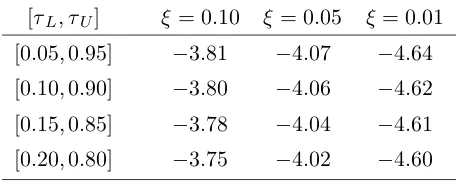
t=1 εt⇒σεW(r). Table 1 reports asymptotic nominal 0.10, 0.05 and 0.01

level critical values for ZAmax_AO for a selection of commonly used trimming parameters. The critical values were obtained by direct simulation of (6), approximating the Wiener processes in the limiting

functionals using N IID(0,1) random variates, with the integrals approximated by normalized sums

of 2,000 steps. Unreported simulations, available from the authors on request, suggest that (i)ZAmax_AO

displays good finite sample size control for all τ0 values, unless a large magnitude break occurs at

τ0 ∈(1/3,2/3) in an extremely large sample, and (ii)ZAmaxAO has attractive power properties underH1,

regardless of whether or not a break is actually present. Given that substantial over-size is only seen

to occur for series that are unrepresentative of those encountered in typical economic applications, a

pragmatic case could be made for usingZAmax_AO, although it is difficult to fully justify such an approach, given that the test still has asymptotic size approaching one whenτ0∈(1/3,2/3).

Table 1. Asymptoticξ-level critical values for theZAmax_AO test [τL, τU] ξ = 0.10 ξ = 0.05 ξ= 0.01

[0.05,0.95] −3.81 −4.07 −4.64

[0.10,0.90] −3.80 −4.06 −4.62

[0.15,0.85] −3.78 −4.04 −4.61

[0.20,0.80] −3.75 −4.02 −4.60

Acknowledgment

Financial support provided by the Economic and Social Research Council of the United Kingdom

References

Alexeev, V. and Maynard, A. (2012). Localized level crossing random walk test robust to the presence

of structural breaks. Computational Statistics and Data Analysis 56, 3322-3344.

Banerjee, A., Lumsdaine, R. and Stock, J. (1992). Recursive and sequential tests of the unit root and

trend break hypotheses: theory and international evidence. Journal of Business and Economics

Statistics 10, 271-288.

Kim, D. and Perron, P. (2009). Unit root tests allowing for a break in the trend function at an

unknown time under both the null and alternative hypotheses. Journal of Econometrics 148,

1-13.

Leybourne, S.J. (1995). Testing for unit roots using forward and reverse Dickey-Fuller regressions.

Oxford Bulletin of Economics and Statistics 57, 559-571.

Perron, P. (1989). The great crash, the oil price shock, and the unit root hypothesis. Econometrica

57, 1361-1401.

Perron, P. (1997). Further evidence of breaking trend functions in macroeconomic variables. Journal

of Econometrics 80, 355-385.

Perron, P. and Zhu, X. (2005). Structural breaks with deterministic and stochastic trends. Journal

of Econometrics 129, 65-119.

Pitarakis, J.-Y. (2012). A joint test for structural stability and a unit root in autoregressions.

Computational Statistics and Data Analysis, forthcoming.

Stock, J.H. and Watson, M.W. (1996). Evidence on structural instability in macroeconomic time

series relations. Journal of Business and Economic Statistics 14, 11-30.

Stock, J.H. and Watson, M.W. (1999). A comparison of linear and nonlinear univariate models

for forecasting macroeconomic time series. Engle, R.F. and White, H. (eds.), Cointegration,

Causality and Forecasting: A Festschrift in Honour of Clive W.J. Granger, Oxford: Oxford

University Press, 1-44.

Stock, J. and Watson, M.W. (2005). Implications of dynamic factor analysis for VAR models, NBER

Working Paper #11467.

Vogelsang, T.J. and Perron, P. (1998). Additional tests for a unit root allowing the possibility of

breaks in the trend function. International Economic Review 39, 1073-1100.

Zivot, E. and Andrews, D.W.K. (1992). Further evidence on the great crash, the oil-price shock, and

Appendix: Proof of Theorem 1

In what follows we can set µ=β = 0 without loss of generality. When τ 6=τ0 we have

T−2PT

t=1yt=T

−2PT

t=1ut+κσεT

−2PT

t=τ0T+1(t−τ0T) p

→κσε(1−τ0)2/2,

T−3PT

t=1tyt=T−3PTt=1tut+κσεT−3PTt=τ0T+1t(t−τ0T) p

→κσε(1−τ0)2(2 +τ0)/6,

T−3PT

t=τ T+1(t−τ T)yt = T

−3PT

t=τ T+1(t−τ T)ut+κσεT

−3PT

t=τ T+1(t−τ T)DTt(τ0) p

→ κσε[{1−τ0−Iττ0(τ−τ0)}2{2 +τ0−3τ + 4Iττ0(τ −τ0)}]/6.

Examining the limit behaviour of the residuals ˆut we obtain



  

T−1µˆ ˆ β ˆ γ     =    

1 T−2PT

t=1t T

−2PT

t=τ T+1(t−τ T)

T−2PT

t=1t T−3

PT

t=1t2 T−3

PT

t=τ T+1t(t−τ T)

T−2PT

t=τ T+1(t−τ T) T

−3PT

t=τ T+1t(t−τ T) T

−3PT

t=τ T+1(t−τ T)2

    −1 ×    

T−2PT

t=1yt

T−3PT

t=1tyt

T−3PT

t=τ T+1(t−τ T)yt

    p →    

1 1₂ (1−₂τ)2

1 2

1 3

(1−τ)2(2+τ) 6 (1−τ)2

2

(1−τ)2(2+τ) 6

(1−τ)3 3



  

−1

  

κσε(1−τ0)2 2 κσε(1−τ0)2(2+τ0)

6

κσε{1−τ0−Iττ₀(τ−τ0)}2{2+τ0−3τ+4Iττ₀(τ−τ0)} 6



  

= :κσε

    P1 P2 P3     giving

T−1uˆbrTc = T−1ybrTc−T−1µˆ−T−1βˆbrTc −T−1γˆIrτ(brTc − bτ Tc)

= T−1ubrTc+κσεIrτ0(r−τ0)−T−1µˆ−βrˆ −γˆIrτ(r−τ) p

→ κσε{Irτ0(r−τ0)−P1−P2r−IrτP3(r−τ)}=:κσεN(r, τ0, τ).

We also require

∆ˆut = ∆yt−βˆ−ˆγDUt(τ)

= κσεDUt(τ0) + ∆ut−βˆ−γDUˆ t(τ)

PT

t=2∆ˆu 2

t = κ2σ2ε(T−τ0T) +PT_t=2∆u2t + (T−1)ˆβ 2

+ ˆγ2(T −τ T)

+2κσεPTt=τ0T+1∆ut−2κσε(T −τ0T)ˆβ−2κσεγˆPTt=2DUt(τ0)DUt(τ)

−2ˆβPT

t=2∆ut−2ˆγPTt=τ T+1∆ut+ 2ˆβγˆ(T−τ T)

T−1PT

t=2∆ˆu2t p

→ σ2_ε[1 +κ2{(1−τ0) +P22+ (1−τ)P32−2(1−τ0)P2−2(1−τ0−Iττ0(τ −τ0))P3

and

Tφˆ= T

−2_uˆ2

T −T−2uˆ21−T−2

PT

t=2∆ˆu2t

2T−3PT

t=2uˆ2t−1

p

→ N(1, τ0, τ)

2_{−N(0, τ} 0, τ)2

2R1

0 N(r, τ0, τ)2dr

.

Now we can establish the limit of ˆσ2_ε

ˆ

σ2_ε = T−1PT

t=2ˆε2t

= T−1PT

t=2∆ˆu 2 t +T2φˆ

2

T−3PT

t=2uˆ 2

t−1−2TφTˆ −2

PT

t=2∆ˆutuˆt−1

p

→ σ2_ε{1 +κ2L(τ0, τ)}+

"

N(1, τ0, τ)2−N(0, τ0, τ)2

2R1

0 N(r, τ0, τ)2dr

#2

κ2σ2_ε

Z 1

0

N(r, τ0, τ)2dr

−2 "

N(1, τ0, τ)2−N(0, τ0, τ)2

2R1

0 N(r, τ0, τ)2dr

#

{κ2σ2_εN(1, τ0, τ)2−κ2σ2εN(0, τ0, τ)2}

= σ2_ε 1 +κ2

"

L(τ0, τ)−

{N(1, τ0, τ)2−N(0, τ0, τ)2}2

2R1

0 N(r, τ0, τ)2dr

#!

=:σ2_ε{1 +κ2M(τ0, τ)}.

It then follows using standard theory that

T−1/2t_φˆ =

T−2uˆ2_T −T−2uˆ2₁−T−2PT

t=2∆ˆu2t

2 q

ˆ

σ2_εT−3PT

t=2uˆ2t−1

p

→ κ

2_{{N(1, τ}

0, τ)2−N(0, τ0, τ)2}

2 q

κ2_{{1 +κ}2_M(τ 0, τ)}

R1

0 N(r, τ0, τ)2dr