Dynamic Benchmark Targeting
∗
Karl H. Schlag
University of Vienna
‡Andriy Zapechelnyuk
University of Glasgow
§February 22, 2017
Abstract
We study decision making in complex discrete-time dynamic environments where Bayesian optimization is intractable. A decision maker is equipped with a finite set of benchmark strategies. She aims to perform similarly to or better than each of these benchmarks. Furthermore, she cannot commit to any decision rule, hence she must satisfy this goal at all times and after every history. We find such a rule for a sufficiently patient decision maker and show that it necessitates not to rely too much on observations from distant past. In this sense we find that it can be optimal to forget.
Keywords: Dynamic consistency, experts, regret minimization, forecast com-bination, non-Bayesian decision making.
JEL classification numbers: C44, D81
∗The authors thank Olivier Gossner, Sergiu Hart, Sebastian Koch, and G´abor Lugosi for valuable
comments. Karl Schlag gratefully acknowledges financial support from the Department of Economics and Business of the Universitat Pompeu Fabra, Grant AL 12207, and from the Spanish Ministerio de Educacion y Ciencia, Grant MEC-SEJ2006-09993.
‡Department of Economics, University of Vienna, Hohenstaufengasse 9, 1010 Vienna, Austria. E-mail: [email protected].
§Corresponding author. Adam Smith Business School, University of Glasgow, University Avenue,
1
Introduction
We are concerned with decision making in discrete-time dynamic environments that
are hard to predict and to model explicitly, due to complexity or lack of information.
How would a firm optimally choose its inventories if the demand for its product is stochastic and subject to unpredictable structural breaks?
How would a police department decide about the number of police cars and their patrol routes if crimes do not follow any stationary pattern?
How should patients in an emergency ward be assigned to doctors if there is no dis-cernible system in arrival of patients with different urgency of medical attention?
In economics, the standard approach to dynamic decision making involves modelling
the environment as a specific stochastic process and then optimizing within this model.
Unknown parameters of the process are estimated by statistical methods. However,
this approach typically comes with several problems. Different assumptions on the
underlying stochastic process lead to different solutions, and the true environment is
never known. Explicit and tractable solutions only exist for simplest scenarios.
Com-plex models that include more realistic features, such as structural breaks at unknown
time, easily make the problem intractable. Tractable models often cannot approximate the real environment, resulting in serious errors in decision making.
An alternative approach that is popular in machine learning considers decision making
with expert advice and the well known no-regret problem.1 It can deal with
envi-ronments of arbitrary complexity—in fact, the modeller does not even need to know
anything about the environment. In this approach, the decision maker is equipped with
a finite set of benchmark strategies or experts that she uses as targets. Her objective
is to perform similarly to or better than each of them, without making any specific
assumptions about the environment. These benchmark strategies could be simple
heuristic decision making rules, standard practices in the given situation, solutions to
the problem under specific assumptions about the environment, or strategies of experts
who know more about the environment than the decision maker does. However, this
approach has two caveats from an economist’s point of view. First, a decision maker is
infinitely patient, there is no discounting of payoffs in practically all papers. Second,
the decision maker has the power to commit to a decision rule, as the performance is
only measured at the outset.
This paper addresses these two caveats by inserting a new pair of elements into decision
making with expert advice: discounting of future payoffs anddynamic consistency. We refer to our methodology asdynamic benchmark targeting. We design a decision-making rule that dynamically combines benchmark strategies and achieves a similar or superior
present-value performance to each of them in all environments, at each point of time,
provided the decision maker is sufficiently patient.
Freedom of choice and the absence of legal instutions that hardwire the behavior make
dynamic consistency a necessity. Dynamic consistency, while being a standard
as-sumption for economists (see Strotz, 1956; Rubinstein, 1998), is a novel feature that our paper introduces to the literature on decision making with expert advice. A
de-cision rule is dynamically consistent if it performs well at any point in time, not only
ex-ante. The decision maker does not commit to any course of actions from the start.
She asks herself in every period, after every history, whether the previously chosen
strategy will continue to perform well enough relative to the set targets and whether
she should continue using it. However, all the literature on decision making with
ex-pert advice assumes commitment to a particular strategy from the start, and thus
ignores dynamic consistency.2 All but two decision rules used in this literature are not
dynamically consistent. The two exceptions are discussed at the end of this section.
Discounting of future payoffs is the paradigm in economic decision making in which one
is forward-looking and considers tradeoffs over time. The literature on decision making
with expert advice considers a backward-looking decision maker concerned with sums
or simple averages of payoffs. The two exceptions are Fudenberg and Levine (1999)
and Olszewski and Peski (2011) that study decision makers who care about future
discounted payoffs, but assume commitment to a particular strategy from the start,
thus ignoring dynamic consistency.
Having both features, dynamic consistency and discounting of future payoffs, makes Blackwell’s Approachability Theorem (Blackwell, 1956) and its extensions (Lehrer,
2003; Lehrer and Solan, 2009) inapplicable. A different method has to be used in this
case.
2Some papers consider infinitely patient decision makers who care about long-run average streams
We show that dynamic consistency is intimately linked to the ability to react to recent
changes in the environment. When evaluating past performance, a dynamically consis-tent decision rule must not place the same weight on all past events, recent and distant
alike. Instead, recent periods should carry a greater weight, as if one gives recent
events more attention. There are many ways to accomplish that, such as assignment
of exponentially decaying weights, equal wights with bounded recall, or equal weights
with periodic restarts by forgetting all past information. It turns out that there is a
strategy that provides better results, both numerically and asymptotically. It requires
the decision maker to have a bounded recall, m, and in every period t to average out
the payoffs over lastktperiods, where eachktis an independent and uniformly random
draw from {1, ..., m}. The recall length m is chosen by the decision maker. We de-rive an optimal length of recall and show that the achieved performance is arbitrarily
close to that of the best benchmark strategy, provided the decision maker is sufficiently
patient. Importantly, we provide an upper bound on how close the decision maker’s
performance is to the best benchmark, for discount factors bounded away from one.
Infinite patience is a simplifying model of someone who is very patient or who looks
far ahead. In the context of this paper we discover that being very patient cannot be
approximated by infinite patience. There is a discontinuity as the discount factor tends
to one, as we further comment on in Section 4.
Related Literature. The problem of outperforming in hindsight a given set of
benchmark strategies, or the no-regret problem, was first considered by Hannan (1957). A substantial literature revisited the problem and offered solutions for a variety of
applications. This methodology is used, among other things, to combine competing
forecasting models (Foster and Vohra, 1993, 1999; Littlestone and Warmuth, 1994),3 to
design investment portfolios and derive bounds on the prices of financial instruments
(DeMarzo et al., 2006, Chen and Vaughan, 2010), to investigate learning in games
(Fu-denberg and Levine, 1995; Freund and Schapire, 1999; Hart and Mas-Colell, 2000, 2001)
and to compute efficient algorithms for job scheduling (Mansour, 2010), online routing
and shortest paths problems (Takimoto and Warmuth, 2003; Blum et al., 2006).4 In
the above literature, a decision maker commits to a decision rule in the initial period.
3For an overview of the forecast combination literature see Timmerman (2006) and Clemen and
Winkler (2007).
In this paper we investigate what happens if the decision maker does not have the
power to commit, and hence is tempted to change the rule at later points in time.
Strategies with diminishing weights on past observations have been introduced in the
literature, but without concern neither for dynamic consistency, nor for optimization of
the discounted sum of future payoffs. Cesa-Bianchi and Lugosi (2006, Ch. 2.11)
eval-uate the past regret as a sum of past single-period regrets with diminishing weights
and show that the past regrets can vanish if and only if the sum of the weights
di-verges. Lehrer and Solan (2009) consider a decision maker who periodically erases her
memory, and show that no regret can be achieved with a sequence of strategies with
bounded recall. While Cesa-Bianchi and Lugosi (2006) and Lehrer and Solan (2009)
only consider performance from the ex-ante perspective, we show that their strategies are dynamically consistent. However, the aim of our paper is not a mathematical proof
of existence, but a formulation of methodology and design of a decision rule with good
properties. Our rule provides a bound on the performance that is superior to those
that we derive for the rules of Cesa-Bianchi and Lugosi (2006) and Lehrer and Solan
(2009).
Our paper also connects to the psychology and experimental literature that documented
the so-calledrecency effect, according to which more distant events are regarded as less relevant.5 In the forecast combination literature, the recency effect, manifested as
diminishing weights on past events, have been used as a heuristic or empirical per-formance improvement tool, e.g., Bates and Granger (1969), Winkler and Makridakis
(1983), Timmerman (2006), S´anchez (2008), and Mallet et al. (2009). In this paper we
identify a novel strategic reason for the recency effect (Section 4).
2
Example
For illustration, let us consider the inventory control problem. Even though our ex-ample is simple and stylized, it has enough structure to demonstrate how difficult and
complex it would be to solve it by standard economic methods. The example shows
how our approach tackles the problem while disregarding its complexity.
5This goes back at least to Watson (1930) and Guthrie (1952). See, e.g., Roth and Erev (1995),
A retailer decides what quantity of a product to hold in stock at the beginning of each
day t = 1,2, . . . The product can be restocked every morning for free, but overnight storage of unsold goods is costly. The daily demand for the product, qt, follows a
stochastic process that we make no assumptions about. The tradeoff is that a larger
stock in the morning means more profit in a day with high demand, but more storage
cost in a day with low demand. As usual in business decision making, the retailer’s
strategy can be adjusted any time. Therefore, it is necessary to consider dynamically
consistent decision rules.
There are three parameters: a per-unit profit from salesπ, a per-unit cost of overnight
storage c, and an annual interest rate r. Denote by st the stock at the beginning of
day t (after the restocking has taken place) and letyt= min{st, qt}be the daily sales.
Thenst−ytis the amount of goods left overnight. The retailer’s profit in day t is thus
πyt−c(st−yt).
The performance evaluated at day t0, measured as the normalized present value of
future profits, is
Πt0 = (1−δ)
∞
X
t=t0
δt−t0 πy
t−c(st−yt)
,
where δ is the daily discount factor, δ =e−r/365.
The standard approach to this problem requires specific assumptions about the
stochas-tic process {qt}that determines demand. Since nothing is known about the stochastic
process, any specific assumptions may be unwarranted, resulting in an inadequate
so-lution. Moreover, if the stochastic process is not ergodic, tractability can become a problem. For instance, this is the case when there are structural breaks in demand
occurring at unknown points in time.
Our approach circumvents these difficulties. Instead of focusing on the environment,
the retailer focuses on a few benchmark strategies that are candidates for being “good”
decision rules. Her aim is to perform similar to or better than each of them.
One such benchmark could be, for example, the fixed quantity system that dictates to restock daily up to a fixed quantity s0 > 0. Another such benchmark could be the
based on past data.
We design a decision rule that performs in any environment similarly to or better than each of these two benchmarks. In particular, if the true environment is i.i.d., in which
case the fixed quantity system is optimal, then our rule will approximately follow the
fixed quantity system. If instead the environment turns out to be Markov, where the
replenishment system performs well, then the retailer will also performs well by using
our rule.
In reality, benchmarks perform differently at different points of time. Our decision
rule tracks which one performs better and keeps the retailer’s performance within a
small errorεof that at all times. It does so by balancing between the two benchmarks,
combining their actions with dynamically adjusted weights that depend on the bench-marks’ past performance, as described in Section 3.2 below. In particular, it is enough
that one of the benchmarks performs well in order to guarantee good profits with our
rule.
How well does our rule perform? Clearly we cannot expect such a benchmark combining
rule to perform better than all the benchmarks. We show that our rule may perform
worse than the best benchmark, but only by a fairly small amount called the error
bound. For example, let the annual interest rate be 5%, so the daily discount factor is δ=e−0.05/365 ≈0.999863. According to our formula (3) in Section 3.2, the error bound of our rule is 4.3% of the daily profit range.6 So, the present value of the retailer’s
future profits is guaranteed, at any time, to be at least as much as that of the best
benchmark strategy minus 4.3% of the daily profit range.
3
Dynamic Benchmark Targeting
3.1
Model
We now introduce the formal model of benchmark targeting. A decision maker takes
actions in discrete time periodst= 1,2, .... In each periodtthe decision maker chooses an action at from a set A of available actions. Then, a state of environment, ωt ∈ Ω,
6Our decision rule’s actions are convex combinations of actions dictated by the benchmarks, so the
maximum stockst can never exceed ¯s. Hence, the daily profit is within [−c¯s, πs¯], and the maximum
is realized and observed by the decision maker. The decision maker’s payoff in that
period depends on bothat and ωt and is denoted byu(at, ωt).
In each periodt, before the decision maker makes her choice, she is provided with
rec-ommendations ofn benchmark strategies. Each benchmark strategy i recommends an
actionrt(i)∈A. Then, the decision maker chooses an actionat ∈Aas a function of the
benchmark recommendations rt(1), ..., rt(n), as well as all past states and
recommen-dations. These benchmarks could be simple heuristic decision making rules, standard
practices in the given situation, solutions to the problem under specific assumptions
about the environment, or experts who know more about the environment than the decision maker does. The important assumption is that benchmark recommendations
do not depend on choices of the decision maker.
We make the following assumptions. The set of actions A is a convex and compact
subset of Rd, d ≥ 1. The payoff function u is uniformly bounded, w.l.o.g. u(a, ω) ∈
[0,1]. In addition, u(a, ω) is concave in a for every ω ∈ Ω.7 The state space Ω is a
compact space (finite or infinite). The sequence of states of environment, ¯ω={ωt}∞t=1,
is arbitrary. For example, it can be determined by a discrete-time stochastic process,
which we make no assumptions about.
The profile of a realized state of the environment and the actions recommended by the
n benchmarks in period t is denoted by xt = (ωt, r1,t, . . . , rn,t) and called an event in
period t. Let ht = (x1, . . . , xt) be the history of the events up to period t and let H
be the set of all finite histories, including the empty history. For each i = 1, . . . , n, a
benchmark strategy is described by a mappi :H →Athat associates with every history
ht−1 an actionrt(i) inA. Adecision rule of the decision maker is a mapp:H×An →A
that associates with every history ht−1 and every profile of current recommendations
rt= (rt(1), . . . , rt(n)) an action rt inA to be chosen in period t.
In what follows, for a given set of benchmark strategies p1, ..., pn and a given decision
rule p, we write for each periodt
rt= p1(ht−1), ..., pn(ht−1)
and at=p(ht−1, rt).
These notations permit two interpretations ofrtthat are equivalent for our purpose.
Ei-7The convexity ofAand concavity ofuin the action implies that every mixed action (lottery over
ther the decision maker knows benchmark strategies (p1, ..., pn), and hence can deduce
their recommendations, or she directly observes the recommendations of the bench-marks and does not need to know their strategies.
For a given sequence of states, ¯ω ={ωt}∞t=1, the performance of a decision rulep from
the perspective of period t0 is measured as the (normalized) discounted sum of future
payoffs that this decision rule delivers,
Ut0(p,ω) = (1¯ −δ)
X∞
t=t0
δt−t0u(a
t, ωt), (1)
where δ ∈ (0,1) is the decision maker’s discount factor. The performance of each
benchmark i from the perspective of period t0 is the discounted sum of future payoffs
that the decision maker can obtain by always following the recommendations of i,
Ut0(pi,ω) = (1¯ −δ)
X∞
t=t0
δt−t0u(r
t(i), ωt).
We now introduce “dynamic benchmark targeting.” The decision maker wishes to
guar-antee the performance within a given error bound of, or better than, the performance
of each benchmark strategy, under each possible sequence of states, and from
perspec-tive of each period of time. “Benchmark targeting” refers to the decision maker’s goal
to outperform all the benchmarks in a given set, allowing only a limited error margin.
“Dynamic” refers to the dynamic consistency of the objective of being within the same
error bound after every possible past history.8
Definition 1. A decision rule p for dynamic benchmark targeting w.r.t. benchmark strategies p1, . . . , pn has error bound ε if
Ut0(p,ω)¯ ≥ max
i∈{1,...,n}Ut0(pi,ω)¯ −ε (2)
for all periods t0 = 1,2, ...and for all sequences of states ¯ω.
Note that condition (2) is a sure inequality that has to hold for every realized sequence
of states. Performance measures Ut0(·,ω) are not expected utilities, these are the¯
8This objective is analogous to theε-sequential optimality notion, orε-subgame perfect equilibrium
discounted sums of the future payoffs that will be realized under the given sequence of
states ¯ω.
We assume that past states are observable. Thus, the decision maker can calculate in
retrospect for each period in the past what she would have achieved with each action.
In fact, for our results to hold, observability of past states is unnecessary, so long as the decision maker can observe her (foregone) payoffs that she would have received if
she had followed any particular benchmark.9
For clarity of exposition we have assumed that each benchmark i’s recommendation
is a deterministic function pi(ht) of past states (and benchmark recommendations).
Our model can deal with arbitrary sequences of states and recommendations, where
a recommendation in each period is simply an action. No assumptions are necessary
about how they are generated. In particular, such sequences can be realizations of a
stochastic process where states and benchmark recommendations are interdependent.
However, an important assumption is that these sequences of states and
recommenda-tions are exogenous to the decision maker’s problem and do not depend on the choices
made by the decision maker. Otherwise, a decision rule with a small error bound need
not exist, because some actions of the decision maker may trigger an irreversible change in all future payoffs.10
3.2
Decision Rule
We now introduce a simple decision rule for dynamic benchmark targeting and then
present an error bound that shows how close it can track the best benchmark at
any point in time. According to this decision rule, in each round the decision maker
chooses a convex combination of the recommendations of the n benchmark strategies.
The benchmarks that made better past recommendations receive greater weights.
9Actually, it suffices to have unbiased estimates of payoffs of each benchmark in each period.
Everything goes through after replacement of realized performance by expected performance. We use this insight in Section 5 to apply our methodology to the case where only payoffs from chosen actions are observed.
10For example, consider the problem with two states, Ω ={0,1}, where the decision maker aims
to guess the state in each period, u(at, ωt) = 1− |ωt−at|, at ∈ A = [0,1]. The nature picks ω1∈ {0,1}, equally likely. If the decision maker has guessesω1 correctly, then the nature repeats the
Fix a periodtwith a historyht−1. For each benchmarkidenote byCt,k(i) the aggregate
payoff over the last k≥1 periods,
Ct,k(i) =
Xt−1
s=t−ku(rs(i), ωs),
where we define u(·, ωs) = 0 for all s ≤ 0, i.e., all payoffs prior to the first period are
set equal to zero. Let Ct,0(i) = 0. Define for k ≥0 thek-score of each benchmarki as
the logistic weight of these aggregate payoffs,
λt,k(i) =
eηCt,k(i)
Pn
j=1eηCt,k(j)
,
whereη ≥0 is a parameter. Then compute the average of k-scores of each benchmark
i for k from 0 to m−1, m1 Pm−1
k=0 λt,k(i), where m is an integer parameter. Note that
the average scores of all benchmarks add up to one. The decision rule p(m,η) that
depends on m and η combines the benchmark recommendations by assigning to each
recommendationrt(i) the weight equal to i’s average score,
p(m,η)(ht−1, rt) = n X
i=1
1 m
m−1
X
k=0
λt,k(i) !
rt(i).
In this way the agent chooses a convex combination of the recommendations.
The decision rule has two free parameters,m and η. The value m−1 is the maximal
number of previous periods that are included in the performance evaluation, whereasη
is a sensitivity coefficient used in the logistic formula. We choose these free parameters to optimize the order of convergence of the error bound asδ approaches 1.
Theorem 1. For a discount factor δ ∈(0,1) let
η= 243 (lnn) 1
3 (1−δ) 1
3 and m= η
2(1−δ)+x,
wherex∈(−1,1]is the adjustment such thatmis an even integer. Decision rule p(m,η)
has error bound
ε = 3
4 2(1−δ) lnn
13
+ 7
96 2(1−δ) lnn
23
. (3)
Note that ε → 0 as δ → 1. Hence, if the decision maker is sufficiently patient, or if
the interval between two consecutive periods is small, then the decision maker can be guaranteed to perform arbitrarily close to, or better than, the best benchmark strategy,
from the perspective of any period.
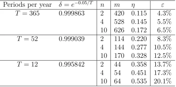
Periods per year δ=e−0.05/T n m η ε
T = 365 0.999863 2 420 0.115 4.3%
4 528 0.145 5.5%
10 626 0.172 6.5%
T = 52 0.999039 2 114 0.220 8.3%
4 144 0.277 10.5%
10 170 0.328 12.5%
T = 12 0.995842 2 44 0.358 13.7%
4 54 0.451 17.3%
[image:12.595.149.451.210.359.2]10 64 0.535 20.1%
Table 1: Numerical percentage values of the error bound.
Our error bound and the optimal parametersm and ηare easily computed for specific
values of δ and n. Table 1 demonstrates the numerical value of the error bound for
the case of annual interest rate r = 0.05 and payoffs evaluated daily (δ =e−0.05/365 ≈
0.999863), weekly (δ = e−0.05/52 ≈ 0.999039) and monthly (δ =e−0.05/12 ≈ 0.995842), with the number of benchmarksn = 2, 4, and 10. As evident from (3) and illustrated
numerically by Table 1, the magnitude of the value of 1−δ(or the frequency of periods
T) plays an exponentially greater role on the size of the error bound, as compared to
the number of benchmarksn. Doubling (1−δ) has the same effect on the error bound
as makingn squared.
3.3
Comparison to Other Decision Rules
The decision rule p(m,η) defined in the previous section performs well when δ is large.
One wonders whether alternative, possibly even simpler rules perform similarly. In this
section we present the error bounds of a few alternative rules. Then, in the next section,
we proceed to derive general necessary properties of rules with low error bounds.
Let Bt(i) denote the evaluation of the past performance of each benchmark i. We
ex-ponential weights of their past performances Bt(i),
q(ht−1, rt) = n X
i=1
eηBt(i)
Pn
j=1eηBt(j)
!
rt(i). (4)
These four rules use the same formula (4) to combine benchmarks, but differ in how
they evaluate benchmark past performance, Bt(i).
First, consider the exponentially weighted average forecaster rule introduced in Little-stone and Warmuth (1994). This rule aggregates all past payoffs from the start for
each benchmark i,
Bt(i) =
Xt−1
s=1u(rs(i), ωs). (5)
This rule has the error bound at least 1/2. In fact, in Section 4 we prove a more general
result that any decision rule that relies “too much” on the distant past will have a
large error bound (Theorem 2). Such decision rules include, among others, calibrated
forecasting of Foster and Vohra (1993, 1999), smooth fictitious play of Fudenberg and
Levine (1995), and regret matching of Hart and Mas-Colell (2000, 2001).
As a good decision rule must focus on the recent past, a natural candidate is the rule
that aggregate payoffs only over the last m periods for a fixed parameter m,
Bt(i) =
Xt−1
s=t−mu(rs(i), ωs).
This rule is not satisfactory either, since its error bound is bounded away from zero.
It does not converge to zero as δ → 1. It is possible to construct an example, as in
Zapechelnyuk (2008), where the decision maker’s and benchmarks’ performances are
cyclical (the cycle length is a function of the length of recallm), so the decision maker
underperforms relative to some benchmark by a constant that is independent of m.
Another simple possibility is to make the decision maker periodically “forget” the past
and start anew. This periodic-restart rule, considered in Lehrer and Solan (2009),
evaluates the past performance of each benchmark i by its aggregate payoff since the
last restart,
Bt(i) =
Xt−1
s=ρ(t)u(rs(i), ωs),
where restarts occur in periods m, 2m, 3m,..., and ρ(t) = mbt−1
m c denotes the period
defined by (4), where Bt(i) is defined above. We now present an error bound of this
rule.
Proposition 1. For every δ ∈ (0,1) there exists (m, η) such that the periodic-restart rule q¯(m,η) has the error bound
ε= 324/3(lnn)1/3(1−δ)1/3. (6)
The proof is in Appendix B.
Lastly, we consider the decision rule that places exponentially decaying weights to more
distant periods, referred to as the exponential-decay rule,
Bt(i) = t−1
X
s=1
αt−su(rs(i), ωs) (7)
for someα ∈(0,1). This is a special case of Cesa-Bianchi and Lugosi’s (2006, Ch. 2.11)
rule of aggregation of the past performance with diminishing weights.
Denote by ˜q(α,η) the exponential-decay rule defined by (4) with the above choice of
Bt(i). We now determine the error bound of this rule.
Proposition 2. For every δ∈(0,1)there exists (α, η) such that the exponential-decay rule q˜(α,η) has the error bound
ε= 32(lnn)1/3(1−δ)1/3+12(lnn)2/3(1−δ)2/3. (8)
The proof is in Appendix B.
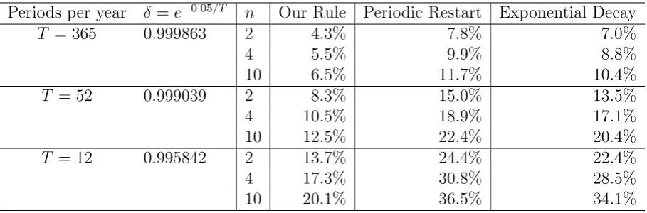
The rates of convergence of the error bounds in Propositions 1 and 2 are the same as
that of our rule p(m,η), but their leading constants are substantially larger. For the
periodic-restart rule the leading constant is 324/3 ≈ 1.717 and for the
exponential-decay rule the leading constant is 32 = 1.5, while the leading constant for our rule is
3 42
1/3 ≈0.945, where 1.717 >1.5>0.945. The error bounds of these two rules are also
compared to the error bound of our rule numerically in Table 2.
Intuitively, the periodic-restart rule performs worse than our rule because of fixed
restart periods. The “adverse” nature can exploit the knowledge of restart periods
Periods per year δ =e−0.05/T n Our Rule Periodic Restart Exponential Decay
T = 365 0.999863 2 4.3% 7.8% 7.0%
4 5.5% 9.9% 8.8%
10 6.5% 11.7% 10.4%
T = 52 0.999039 2 8.3% 15.0% 13.5%
4 10.5% 18.9% 17.1%
10 12.5% 22.4% 20.4%
T = 12 0.995842 2 13.7% 24.4% 22.4%
4 17.3% 30.8% 28.5%
[image:15.595.80.535.128.278.2]10 20.1% 36.5% 34.1%
Table 2: Numerical comparison of error bounds of three decision rules.
perform badly when evaluated from the perspective of this period. The idea to avoid
this vulnerability by concealing the periods of restart led to the construction of our
rule.
The reason why our rule performs better than the exponential-decay rule roots in our
method of proof. Our derivation of the error bounds relies on Cesa-Bianchi and Lugosi’s
(2006, Theorem 2.3) tight bound on simple (unweighted) sums of single-period losses.
The uniform distribution of past windows used in our rule translates nicely into simple
sums of losses, whereas it is more difficult to translate the sum of exponentially weighted
losses into weighted simple sums. Another intuitive reason for a better performance
of our rule is its restriction of the number of recent periods involved in making the
next choice. The intuition brought forward in the next section is that sufficiently old
observations should simply be ignored, not even included with exponentially small weights.
4
The Role of Adaptation
In this section we identify necessary conditions for a decision rule to have a low error
bound. We will argue that a key issue in the design of such decision rules is the
appropriate choice of the weights on past information. The error bound ε remains
bounded away from zero as δ → 1 if the decision rule adapts to new information too
fast or too slow. Too much weight on the recent past makes the rule susceptible to
past makes the rule sluggish and unable to track recent changes the performance of
the benchmarks, and hence of which benchmark performs best.
We consider a subclass of decision rules P described as follows. Every rule p ∈ P
chooses an action at each periodtequal to the convex combination of the benchmark’s
recommendations (rt(1), ..., rt(n)),
p(ht−1, rt) = n X
i=1
µt(i)rt(i),
with weights (µt(1), ..., µt(n)) satisfying the following two conditions.
Monotonicity. For each period t and each benchmark i, weightµt(i) is weakly
increas-ing in the past performance of benchmark i, ceteris paribus. Formally, for any two
sequences of states, ¯ω and ¯ω0, that differ only in the payoff of benchmark i in some
period s < t, if us(rs(i), ωs) > us(rs(i), ω0s), then weight µt(i) is weakly greater under
¯
ω than under ¯ω0.
Anonymity. Names of benchmarks do not matter. The weights (µt(1), ..., µt(n)) are
invariant under permutation of indices (1, ..., n).
For each rule in classP we define a measure of adaptivity, that is, the degree to which
the rule adapts to new information, and then show how adaptive a rule has to be in
order to generate a low error bound. Our measure of adaptivity is defined by looking
at sequences in which each benchmark recently only generated the extreme payoffs 0
or 1. We call a rule at most k-adaptive for k ∈ N if it puts a weakly greater weight on benchmarki whenever in the last k periods benchmark ireceived 1 while all other
benchmarks received 0. We call a rule k-adaptive if it is not at most k−1 adaptive. If no such k exists, then the decision rule is called unadaptive. Formally, we say that a decision rule p ∈ P is k-adaptive if k is the smallest integer that satisfies for each periodt ≥k+ 1,
if u(rs(i), ωs) = 1 and u(rs(j), ωs) = 0 for all j 6=iand all s∈ {t−k, ..., t−1}
then µt(i)≥µt(j) for all j 6=i.
Obviously, every monotonic and anonymous decision rule with weights that depend only
the recent m periods is at most m-adaptive. This applies to our decision rule p(m,η)
restarts and Zapechelnyuk’s (2008) rule with a bounded recall window. The decision
rule with exponentially decaying weights (7) is k-adaptive, where k is the median of the exponential distribution, the smallest integer satisfyingPk
s=1α
s ≥P∞ s=k+1α
s. The
exponentially weighted average forecaster rule (5), as well as any rule based on the sum
or simple average of all past payoffs, is unadaptive.
Theorem 2. Every k-adaptive decision rule in P has error bound
ε≥max
1 2(k+1) log(k+1),
1−δk−1
2
.
Every unadaptive decision rule in P has error bound ε≥ 1 2.
The proof is in Appendix A.
Theorem 2 shows that a decision rule whose error bound approaches 0 asδ tends to 1
must necessarily be increasingly adaptive w.r.t.δ, but not too adaptive. The adaptivity
parameter k =k(δ) must diverge as δ →1, but it must grow slower than (lnδ)−1, so
that both bounds, 2(k+1) log(1 k+1) and
1−δk−1
2 , approach zero.
In particular, we uncover a discontinuity at δ = 1. The unadaptive strategies used in
the literature on no-regret and decision making with expert advice that are known to
perform well for an infinitely patient decision maker, such as Littlestone and Warmuth’s
(1994) exponentially weighted average forecaster rule, Hart and Mas-Colell’s (2000)
regret matching, lp-norm strategies of Hart and Mas-Colell (2001) and Cesa-Bianchi
and Lugosi (2003), as well as the smooth fictitious play (Fudenberg and Levine, 1995),
perform very badly when δ is less than, but arbitrarily close to 1.
To obtain these lower bounds, we test a rule against specific environments. First
we explain what can go wrong if too little weight is given on the distant past. The
corresponding bound is ε≥ 1
2(k+1) log(k+1). We obtain this bound by testing a rule in an
i.i.d. environment and evaluating its performance in expectation. Note that any bound
on the expected performance is also a lower bound on the realized performance. When
a rule is k-adaptive, then unlikely sequences of events will be too influential on the
decisions and can steer the rule away the best benchmark.
Consider the following example. There are two possible states of the environment,Rain
1−a. There are two constant benchmarks: one always forecastsRain, the other always forecasts Sun. Suppose that states Rain and Sun occur with probability 1−σ and σ, respectively, independently in every period, σ > 1/2. After k consecutive periods of
Rain ak-adaptive rule will assign the weight at least 1/2 on Rain. The event that such a sequence occurs has a probability exponentially decreasing ink. Yet, this probability
is strictly positive, thus preventing the decision maker from forecasting Sun, which is the best benchmark in expectation.
Next, we argue what can go wrong if too much weight is given on distant past. The
correspondent bound is ε ≥ 1−δk−1
2 for a k-adaptive rule and ε ≥
1
2 for an unadaptive
rule. We explain the intuition by illustrating what can happen with an unadaptive rule
that equally weighs all past information. If some benchmark that has been the best
for a long time becomes inferior, then it may take a very long time for the decision
maker to adjust the weights towards different benchmarks. The longer the history, the
longer it will take to adapt to changes. No matter how patient the decision maker is,
she risks to get stuck with a wrong benchmark for an arbitrarily long period of time.
Thus, the problem of dynamic consistency arises. After some time and some histories the decision maker will prefer to “forget” the past and to restart her decision rule from
the empty history.
For illustration, let us consider the payoffs of the previous example. We now consider
sequences of states and evaluate realized payoffs. Assume that Sun occurs in the first T periods and Rain occurs ever after. Then, in every period t = T + 1, . . . ,2T, the decision maker will assign a weight at most 1/2 on Rain, even though Rain occurs in each of these periods. The payoffs in periods T + 1 to 2T are thus at most 1/2, far
from the best. So, for any given discount factor δ < 1 and a sufficiently large T, the
decision rule’s performance evaluated at period T + 1 is substantially worse than that
of the best benchmark (in this example, the constant benchmark that forecastsRain).
5
Extensions
Within our methodology we can allow for certain extensions of our model.
Non-convex and finite action sets. We show why our results extend to a more
u(a, ω) need not be concave in a. The model where there are only finitely many
different actions is a special case. The challenge that we face here is that for a given vector of benchmarks’ actions, (rt(1), ..., rt(n)), the decision rule p(m,η) stipulates to
choose an action at equal to some linear combination of (rt(1), ..., rt(n)). But at may
not belong toA, since the latter need not be convex. As in Hannan (1957) or Hart and
Mas-Colell (2001), we deal with this problem by letting the decision maker play a mixed
strategy, a lottery over benchmark recommendations, which themselves are elements
of A by definition. Accordingly, the decision maker follows the recommendation of
benchmark i with probability equal to the weight λt(i) assigned on this benchmark in
each period t. All our results then hold in expectation w.r.t. the decision maker’s own mixed strategy.
The multi-armed bandit setting. Consider learning under partial information
where the decision maker observes only payoffs from chosen actions. Payoffs of the
benchmarks whose actions have not been adopted are not observed. Here we explain
how to extend our algorithm to derive the result analogous to Theorem 1.
Since the foregone payoffs are not observed, we use the trick of Auer et al. (1995)
to construct their unbiased estimates. Define the estimate ˆut(i) of a payoff of each
benchmark i in every period t as u(at, ωt)/rt(i) if benchmark i’s action is chosen by
the decision maker in period t, and ˆut(i) = 0 otherwise. Then, in each period with
probability 1−ν use our decision rule p(m,η) w.r.t. the estimated past performances
of the benchmarks, and with probability ν follow the action of a random benchmark,
choosing each benchmark equally likely. These adjustments can be easily accounted
for in our proofs to yield a result as in Theorem 1, the existence of a simple decision
rule for dynamic benchmark targeting. Note that each benchmark is followed with
probability greater or equal toν, hence all estimates are bounded from above by 1/ν.
The parameter ν >0 is called the rate of experimentation, its value can be fine-tuned
for the best performance. Naturally, the new error bound will be greater, as now the
decision maker conditions her decisions on much less information.
Decision makers with bounded horizon. Suppose that a decision maker does not
discount future payoffs, but instead is concerned in each periodt with average payoffs
overt+ 1, . . . , t+T for a fixed horizon T. Here the same simple rule can be used. Some
work is needed to derive a new error bound and then to choose the free parametersm
We hasten to point out that if a decision maker faces a finitely repeated decision
problem in periods t= 1,2, . . . , T, then dynamic benchmark targeting strategies with error bound ε < 1/2 fail to exist, regardless of how past information is used. The
intuition is simple. After facing T −1 periods, the decision maker is only concerned
with her payoff in the final period T. However, the state of the environment in the
last period need not depend on the past realizations. Thus, the decision maker can
guarantee only the maxmin payoff, in ourRain & Sun example in Section 4 this is 1/2, while the payoff of the best benchmark in the final round is equal to 1.
6
Conclusion
In this paper we introduce a methodology for dynamic decision making in which at
each point in time the decision maker compares own performance to a given set of benchmark algorithms, rules of thumb, or advices of experts. The novelty of this paper
is in the addition of a new pair of elements into decision making with expert advice:
discounting of future payoffs and dynamic consistency. We present a decision rule
that guarantees to perform, in terms of discounted present values, nearly as well as or
better than each of these benchmarks at any point in time. Using our rule, the decision
maker need not model the environment, as she would under the Bayesian paradigm,
and hence does not use complicated optimization routines and need not be worried
about misspecifying the environment. Choices are time consistent, hence if the best
benchmark changes, then the decision maker will track this change.
Within our introduced methodology the notion of optimality is well defined, as we
search for a decision rule with the smallest error bound. The bound presented for
our rule (Theorem 1) and for the two alternative rules (Propositions 1 and 2) are not
known to be tight. A topic for future research is to improve these bounds, to find new
rules with better bounds or to design rules and establish bounds for more restricted
environments. The natural first step in this direction is to establish a lower bound on the error bound of any rule.
Notice that the error bound of our rule has been derived for the worst case and depends
only on the number of benchmarks, but not their properties. For a specific choice of benchmarks and for a specific environment the error bound can be much lower. How
future research.
A separate question that this paper does not address is the choice of benchmarks. An additional benchmark can substantially improve performance if it turns out to
per-form much better than the others in the given environment. At the same time, adding
a benchmark potentially increases the error bound, as it is more difficult to
outper-form more benchmarks. So the decision maker has the tradeoff between a potentially
higher absolute performance and a potentially larger gap in performance to the best
benchmark. This is another avenue for future research.
Appendix A. Proofs
A.1
Proof of Theorem 1
Proof. Consider the rulep(m,η) with given parametersm ∈Nand η >0. Recall that
Ct,0(i) = 0, Ct,k(i) = Pt−1
s=t−ku(as(i), ωs) for k ≥ 1, and λt,k(i) = e
ηCt,k(i)
Pn j=1eηCt,k
(j). The
values for t−k ≤0 are well defined by the convention that all payoffs in nonpositive
rounds are zero. The actions of the rule p(m,η) for all t∈N are
at=p(m,η)(ht−1, rt) = n X
i=1
1 m
m−1
X
k=0
λt,k(i) !
rt(i).
Fix a benchmarki∈ {1, ..., n}, a sequence of states ¯ω, and a roundt0. We now bound
the loss from not following that benchmark,Ut0(rt(i),ω)¯ −Ut0(at,ω).¯
For every k = 0,1, ..., m−1 define the rule that combines the benchmarks based on
their performance in the recent k periods,
bt,k = n X
j=1
λt,k(j)rt(j).
Note that for k = 0 the past is ignored and the weights are assigned uniformly to all
By concavity ofu(a, ω) in a and Jensen’s inequality we have
u(at, ωt)≥
1 m
m−1
X
k=0
u(bt,k, ωt). (9)
For eachk = 0,1, ..., m−1 denote byDt,t+k(i) the loss from not following the action of
benchmarki in roundt+k when using the rule bt+k,k based on the recent observations
over rounds in{t, t+ 1, ..., t+k−1},
Dt,t+k(i) =u(rt+k(i), ωt+k)−u(bt+k,k, ωt+k).
We now derive a bound on the sumPm−1
k=s Dt,t+k(i) using the technique of Cesa-Bianchi
and Lugosi (2006, Theorem 2.2) based on Hoeffding inequality (Hoeffding, 1963).
Lemma 1.
m−1
X
k=s
Dt,t+k(i)≤T(s, m) := min
m−s,lnn
η +s+
η
8(m−s)
.
Proof. Since Dt,t+k(i)≤1, we obtain
Pm−1
k=s Dt,t+k(i) ≤m−s. For the second bound
we generalize Theorem 2.2 of Cesa-Bianchi and Lugosi (2006). For i∈ {1, ..., n} let
ws(i) =e−η
Ps−1
k=0Dt,t+k(i)
and let Ws = Pn
i=1ws(i). Note that e−ηs ≤ ws(i) ≤ 1 for all s and all i, so Ws ≤ n.
Thus, for everyi∈ {1, ..., n} we have
lnWm Ws
= ln
n X
j=1
ws(j)e−η
Pm−1
k=s Dt,t+k(j)
!
−lnWs≥ln
ws(i)e−η
Pm−1
k=s Dt,t+k(i)
−lnn
= lnws(i)−η m−1
X
k=s
Dt,t+k(i)−lnn≥ −ηs−η m−1
X
k=s
Dt,t+k(i)−lnn.
Using the following inequality (Cesa-Bianchi and Lugosi, 2006, p. 17)
lnWm Ws
≤ η
2
we obtain
m−1
X
k=s
Dt,t+k(i)≤
lnn
η +s+
η
8(m−s).
Next, by (9) we have
Ut0(rt(i),ω)¯ −Ut0(at,ω) = (1¯ −δ)
∞
X
t=t0
δt−t0(u(r
t(i), ωt)−u(at, ωt)
≤∆ := (1−δ)
∞
X
t=t0
δt−t0 1
m
m−1
X
k=0
Dt−k,t(i).
We can rewrite ∆ as follows,
∆ = 1−δ
m
t0−1
X
t=t0−m+1
δt−t0
m−1
X
s=t0−t
δsDt,t+s(i) +
1−δ m
∞
X
t=t0
δt−t0
m−1
X
s=0
δsDt,t+s(i). (10)
Let us bound the second term in the right-hand side of (10). By Lemma 1,
m−1
X
l=0
Dt,t+l(i)≤
lnn
η +
ηm 8 .
Thus we have
m−1
X
s=0
δsDt,t+s(i) = (1−δ) m−2
X
s=0
δs
s−1
X
l=0
Dt,t+l(i) +δm−1 m−1
X
l=0
Dt,t+l(i)
≤(1−δ)
m−2
X s=0 δs lnn η + ηs 8
+δm−1
lnn η + ηm 8
= lnn
η +
η
8(1−δ)(1−δ
m). (11)
Next, let us deal with the first term in the right-hand side of (10). By Lemma 1,
m−1
X
l=k
Fort∈ {t0−m+ 1, ..., t0−1}setk =t0−t−1. Observe that 0≤k ≤m−2. We have
δt−t0
m−1
X
s=t0−t
δsDt,t+s(i) = (1−δ) m−2
X
s=k
δs−k
s−1
X
l=k
Dt,t+l(i) +δm−1−k m−1
X
l=k
Dt,t+l(i)
≤(1−δ)
m−2
X
s=k
δs−kT(k, s) +δm−1−kT(k, m). (12)
By (11) and (12) we obtain
∆≤Φ(m,η):=
1−δ m
m−2
X
k=0
(1−δ)
m−2
X
s=k
δs−kT(k, s) +δm−1−kT(k, m)
! + 1 m lnn η + η
8(1−δ)(1−δ
m)
. (13)
Since Ut0(rt(i),ω)¯ −Ut0(at,ω)¯ ≤ Φ(m,η) for all benchmarks i, all rounds t0, and all
sequences of states ¯ω, the term Φ(m,η) is an error bound for rule p(m,η).
Next, we make the error bound Φ(m,η) small by choosing the free parameters m andη.
The values that approximately minimize Φ(m,η) are
η∗ = 243 (lnn) 1
3 (1−δ) 1
3 and m∗ = η
∗
2(1−δ)+x. (14)
where x∈ (−1,1] is the adjustment such that m is an even integer. For the proof we do not need to show how these optimal parameters are derived, we only need to prove
that Φ(m∗,η∗) has the stated error bound,
Φ(m∗,η∗)≤ 3
4 2(1−δ) lnn
13
+ 7
96 2(1−δ) lnn
23
. (15)
In order to deal with the inconvenient, nondifferentiable termT(k, s) in (13), we use
T(k, s) = min
s−k,lnn
η∗ +
η∗s 8
≤T˜(k, s) :=
s−k, k ≤ m∗
2 , lnn
η + ηs
8 , k >
m∗
The summations then split into two differentiable parts,
m∗−2
X
s=k
δs−kT(k, s)≤ m∗−2
X
s=k
δs−kT˜(k, s) =
m∗/2
X
s=k
δs−k(s−k) +
m∗−2
X
s=m∗/2 δs−k
lnn
η∗ +
η∗s 8
.
ReplacingT by ˜T in the right-hand side of (13) yields a differentiable expression. Using
the Taylor expansion of this expression w.r.t. (1−δ) up to the third term yields (15),
where the third term of the expansion is nonpositive and bounded by zero.
A.2
Proof of Theorem 2
The theorem is proved by example. Consider two states 0 and 1, set of actions A =
[0,1], and payoffs given byu(a, ω) = 1− |a−ω|, a∈A= [0,1],ω ∈Ω ={0,1}. There
are two benchmarks, labeled 0 and 1, that recommend the respective extreme constant
actions,rt(0) = 0 andrt(1) = 1 for all t.
To prove that the error bound of ak-adaptive decision rule satisfiesε≥ 1
2(k+1) log(k+1), we
consider an i.i.d. environment and compare the expected performance of the benchmark
and a given decision rule. Note that a lower bound on the difference in the expected
performance is also a lower bound on the realized performance, for some sequence of
realized events.
Consider the following environment. The state equals 0 and 1 with probability 1−σ
andσ, respectively, independently in all periods,σ ∈(12,1). In this setting, benchmark
1 is the better of the two as it is correct with probability σ > 12 in every period and
yields the expected payoffE[u(1, ω)] =σ.
For each period t > k let Et be the event that ωt−s = 0 for every s = 1, . . . , k. Since
we have assumed u(a, ω) = 1− |a−ω|, under event Et we have u(0, ωt−s) = 1 and
u(1, ωt−s) = 0 for each s = 1, . . . , k, and hence µt(0) ≥ µt(1) by k-adaptivity. The
expected payoff of the decision maker conditional on Et is
E[u(p, ωt)|Et] =σ(µt(1)·1 +µt(0)·0) + (1−σ)(µt(1)·0 +µt(0)·1)
=σ−µt(0)(2σ−1)≤σ− 12(2σ−1) = 12,
upper bound on the expected stage payoff isσ, it follows that
E[u(p, ωt)] = E[u(p, ωt)|Et] Pr[Et] +E[u(p, ωt)|not Et](1−Pr[Et])
≤ 1
2Pr[Et] +σ(1−Pr[Et]) = σ−(σ− 1
2) Pr[Et] =σ− 2σ−1
2 (1−σ)
k.
As the expected payoff of benchmark 1 isσ, the difference is
E[u(1, ωt)−u(p, ωt)]≥ 2σ2−1(1−σ)k.
Since the choice ofσ is arbitrary, maximizing the right-hand side w.r.t. σ∈[12,1] yields
max
σ∈[12,1] 2σ−1
2 (1−σ)
k =
k k+ 1
k
1
2k(k+ 1) ≥
1 2(k+1) log(k+1).
Since the state is i.i.d., the expected discounted sum of future payoffs for the
deci-sion maker in every period t > k is also less than benchmark 1’s payoff by at least
1
2(k+1) log(k+1), independently of the discount factor. It is immediate that the same
state-ment is true for some realized path of the events. Consequently, the error bound
satisfies
ε≥ 1
2(k+1) log(k+1).
Next, to prove that the error bound of a k-adaptive decision rule satisfies ε≥ 1−δk−1
2 ,
consider the following environment. Let T be an integer and consider the sequence of
states ¯ω where ωt= 1 for all t≥T.
Then, for every period t = T, T + 1, ..., T +k −2, in the recent t−T < k periods
benchmark 1 has payoff one and benchmark 0 has payoff zero. Hence, byk-adaptivity,
there exists a large enough T and a history of states preceding T such that µt(1) <
µt(0). Moreover, by monotonicity, this history is such that ωs = 0 for all s < T, so
that benchmark 1 is worst and benchmark 0 is best in all periods beforeT. Under this
history,
µt(1) < µt(0) for all t =T, T + 1, ..., T +k−2. (16)
Thus,
UT(p,ω)¯ <(1−δ) k−2
X
s=0
δs(0·1 2 + 1·
1 2) +δ
k−1U
T+k−1(p,ω)¯ ≤
1 2(1−δ
The discounted sum of payoffs of benchmark 1 in period T is UT(p1,ω) = 1, since in¯
all periods from T on benchmark 1’s payoff is constantly one. Hence the error bound must satisfy
ε≥UT(p1,ω)¯ −UT(p,ω)¯ ≥1−
1 2(1−δ
k−1)−δk−1 = 1
2(1−δ
k−1).
Finally, we prove that the error bound of an unadaptive decision rule satisfies ε ≥ 1 2.
Within the same environment considered above, if a decision rule is unadaptive, then
for every k there exists T =T(k) such that (16) holds, and hence
ε≥UT(k)(p1,ω)¯ −UT(k)(p,ω)¯ ≥
1 2(1−δ
k−1).
Since the error bound must satisfy the above for all periods, we have
ε≥sup
k∈N
1 2(1−δ
k−1)
= 1
2.
Appendix B. Proofs (Online Appendix)
B.1
Proof of Proposition 1
Consider a rule ¯q(m,η) for some parameters m ∈ N and η > 0, and fix a sequence of
states ¯ω.
Define Zt(i) = u(rt(i), ωt)− u(at, ωt) for every i = 1, . . . , n and every t. We shall
also simplify notations for the sum of the future discounted payoffs, writing Ut0(0) for
Ut0(¯q(m,η),ω) and¯ Ut0(i) forUt0(pi,ω).¯
for some integer k0. We have
J(i) =Ut0(i)−Ut0(0) = (1−δ)
∞
X
t=mk0
δ(t−mk0)Z
t(i) = (1−δ)
∞
X
k=k0
δm(k−k0)
m−1
X
s=0
δsZmk+s(i)
= (1−δ) ∞
X
k=k0
δm(k−k0)
m−1
X
s=0
(δs−δm−1)Zmk+s(i) + m−1
X
s=0
δm−1Zmk+s(i) !
.
Now, since |Zt(i)| ≤1,
m−1
X
s=0
(δs−δm−1)Zmk+s(i)≤ m−1
X
s=0
(δs−δm−1) = 1−δ
m
1−δ −mδ
m−1.
Also, by Theorem 2.2 in Cesa-Bianchi and Lugosi (2006),
m−1
X
s=0
Zmk+s(i)≤
lnn
η +
mη
8 ≤
r
mlnn
2 ,
where we choose η=p(8 lnn)/m. Hence,
J(i)≤(1−δ) ∞
X
k=k0
δm(k−k0) 1−δ
m
1−δ −mδ
m−1
+δm−1
r
mlnn 2
!
= 1−δ
1−δm
1−δm
1−δ −mδ
m−1
+δm−1
r
mlnn 2
!
= 1− 1−δ
1−δmδ
m−1 m−
r
mlnn 2
!
.
Next, consider any t0 and denote by z ∈ {0,1, ..., m−1} the number of periods that
remain until the next restart, so the integer t0+z is a multiple ofm. Using|Zt(i)| ≤1
and that the sum from the period of restart on isJ(i), we have
Ut0(i)−Ut0(0) = (1−δ)
t0+z−1
X
t=t0
δt−t0Z
t(i) + (1−δ)δz
∞
X
t=t0+z
δt−t0Z
t(i)
= (1−δ)
t0+z−1
X
t=t0
Since J(i) ≤ 1, this expression is increasing in z, so the worst case is z = m −1.
Substituting the bound for J(i), we have
Ut0(i)−Ut0(0) ≤1−δ
m−1+δm−1 1− 1−δ
1−δmδ
m−1 m−
r
mlnn 2
!!
= 1−δ2(m−1) 1−δ
1−δm m−
r
mlnn 2
!
.
Substitutingm=m(δ) = c/(1−δ)2/3 with a parameterc >0 into the above expression, using Taylor expansion up to the second term and upper-bounding that term by zero
yields
Ut0(i)−Ut0(0) ≤
3 2c+
1
√
c
r
lnn 2
!
(1−δ)1/3.
Choosingc to minimize the leading constant, c= 2−1/33−2/3(lnn)1/3, yields
Ut0(i)−Ut0(0) ≤
3 2
4/3
(lnn)1/3(1−δ)1/3.
Since the above holds for each benchmarki and for each starting period t0, the
state-ment of the proposition follows immediately.
B.2
Proof of Proposition 2
Consider a rule ˜q(α,η) for some parameters α ∈ (0,1) and η > 0. Fix a sequence of
states ¯ω and a round t0.
DefineXt(0) = u(at, ωt) and Xt(i) =u(rt(i), ωt) for every i = 1, . . . , n and every t. In
these notations, the performance of every benchmark i= 0,1, . . . , n is evaluated by
Cα,t(i) =Xt(i) +αCα,t−1(i), t ≥1,
withCα,0(i) = 0. We shall also simplify notations for the sum of the future discounted
payoffs, writing Ut0(0) for Ut0(˜q(α,η),ω) and¯ Ut0(i) for Ut0(pi,ω).¯
To begin with, let us show that
Ut0(i)−Ut0(0)≤α
1−δ
1−α +
(1−δα)η
8α(1−α) +
1−δα
Letwt(i) =eηCα,t−1(i), so w1(i) = 1 and
wt+1(i) = wtα(i)eηXt(i), t ≥2 .
Also, letWt = Pn
j=1wt(j) and vt(i) = wWt(ti) for alli= 1, . . . , n and allt≥1. Note that
decision rule ˜q(α,η)stipulates to play in every periodtthe weighted average of the
bench-marks’ recommended actions, with weight vt(i) assigned to the action recommended
by benchmarki= 1. . . , n,
at = n X
i=1
vt(i)rt(i).
By concavity ofu(a, ω) in a and Jensen’s inequality,
Xt(0) ≥ n X
j=1
vt(j)Xt(j). (18)
First, we find a bound on Xt(0). Using Jensen’s inequality again, we obtain
lnWt+1
Wα t = ln n X j=1
wt+1(j)
Wα t = ln n X j=1
wtα(j)
Wα
t
eηXt(j)= ln
n X
j=1
vtα(j)eηXt(j)
= ln
" n X
j=1
vtα(j) e
ηXt(j)
Pn
k=1eηXt(k)
! n X
k=1
eηXt(k)
!#
≤ln
" n X
j=1
vt(j)
eηXt(j)
Pn
k=1eηXt(k)
!α n X
k=1
eηXt(k)
!#
=αln
n X
j=1
vt(j)eηXt(j)+ (1−α) ln n X
j=1
eηXt(j)
=αln
n X
j=1
vt(j)eηXt(j)+ (1−α) ln
1 n
n X
j=1
eηXt(j)
!
+ (1−α) lnn.
We will need the following generalization of the Hoeffding inequality.
Lemma 2 (Cesa-Bianchi and Lugosi 2006, Lemma 2.2). Let Z be a random variable with a≤Z ≤b. Then for every s ∈R,
lnE
esZ
≤sEZ+ s
2(b−a)2
By Lemma 2, inequality (18) and the assumption thatXt(j)∈[0,1],
ln
n X
j=1
vt(j)eηXt(j) ≤η n X
j=1
vt(j)Xt(j) +
η2
8 ≤ηXt(0) + η2
8.
Again, by Lemma 2,
ln 1
n
n X
j=1
eηXt(j)
! ≤ η n n X j=1
Xt(j) +
η2
8 =ηθt+ η2
8 ,
where θt= n1 Pnj=1Xt(j). Consequently,
lnWt+1
Wα
t
≤αηXt(0) + (1−α)ηθt+
η2
8 + (1−α) lnn.
Thus, we have derived
Xt(0)≥
1 αηln
Wt+1
Wα
t
−1−α
α θt−
η
8α −
1−α
αη lnn. (19)
Second, we find a bound on
Cα,t(0) = t X
k=1
αt−kXk(0).
Following (19),
Cα,t(0)≥
1 αη
lnWt+1
Wα
t
+αln Wt
Wα
t−1
+. . .+αt−1ln W2
Wα
1
− 1−α
α
t X
k=1
αt−kθt−
η
8α +
1−α
αη lnn
t
X
k=1
αt−k
= 1
αηln Wt+1
Wα
t
Wtα Wα2
t−1
. . .W
αt−1
2
Wαt
1
−1−α
α
t X
k=1
αt−kθt−
η
8α +
1−α
αη lnn
1−αt 1−α
= 1
αηln Wt+1
Wαt
1
−1−α
α
t X
k=1
αt−kθt−
η 8α
1−αt
1−α −
1−αt
αη lnn
= 1
αηlnWt+1− 1−α
α
t X
k=1
αt−kθt−
η 8α
1−αt
1−α −
where we usedW1 =
Pn
j=1w1(j) = n, so lnWα
t
1 =αtlnn.
Fix anyj = 1, . . . , n. Using Wt+1 =Pkwt+1(k)≥wt+1(j) =eηCt(j), we obtain
Cα,t(0)≥
1
ηlnWt+1+
1−α
αη lnWt+1− 1−α
α
t X
k=1
αt−kθt−
η 8α
1−αt
1−α −
1 αη lnn
≥Cα,t(j) +
1−α
αη lnWt+1−η
t X
k=1
αt−kθt !
− η
8α 1
1−α −
1 αη lnn.
Observe that
lnWt+1−η
t X
k=1
αt−klnθt = ln n X
j=1
eηPtk=1α
t−kX k(j)−
t X
k=1
αt−k1 n
n X
j=1
Xk(j)
= lnn+ ln 1
n
n X
j=1
ey(j)
! − 1 n n X j=1 y(j),
where y(j) =ηPt k=1αt
−kX
k(j). By Jensen’s inequality,
1 n
n X
j=1
ey(j) ≥e1n Pn
j=1y(j),
and hence
lnWt+1−η
t X
k=1
αt−klnθt ≥lnn+ ln
e1n Pn
j=1y(j)
− 1 n n X j=1
y(j) = lnn.
Consequently,
Cα,t(0)≥Cα,t(j) +
1−α
αη lnn−
η
8α(1−α) −
1 αηlnn
=Cα,t(j)−
η
8α(1−α)−
lnn
Finally, we bound Ut0(0). We evaluate for j ∈ {0,1, .., n},
(1−δ) ∞
X
t=t0
δt−t0C
α,t(j) = (1−δ)
∞
X
t=t0
δt−t0
t X
k=1
αt−kXk(j)
= (1−δ) (α
t0−1+δαt0 +δ2αt0+1+...)X
1(j) + (αt0−2+δαt0−1+...)X2(j)
+..+ (1 +δα+...)Xt0(j) + (δ+δ
2α+...)X
t0+1(j)...
!
= (1−δ) α
t0−1(1 +δα+δ2α2+...)X
1(j) +αt0−2(1 +δα+...)X2(j)
+..+ (1 +δα+...)Xt0(j) +δ(1 +δα+...)Xt0+1(j) +...
!
= (1−δ) 1
1−δα ∞
X
t=t0
δt−t0X
t(j) + (1−δ)
1 1−δα
t0−1
X
k=1
αt0−kX
k(j)
= 1
1−δαUδ,t0(j) +
1−δ 1−δα
t0−1
X
k=1
αt0−kX
k(j).
Using (20) we obtain
Ut0(j)−Ut0(0)
1−δ = (1−δα)
∞
X
t=t0
δt−t0[C
α,t(j)−Cα,t(0)]− t0−1
X
k=1
αt0−k[X
k(j)−Xk(0)]
≤ 1−δα
1−δ
η
8α(1−α)+
lnn η
+
t0−1
X
k=1
αt0−k
= 1−δα
1−δ
η
8α(1−α) +
lnn η
+α1−δ 1−α,
which completes the proof of (17).
Next, chooseα and η that satisfy
1−α
α =
2 (1−δ)2/3
(lnn)1/3
andη = 2p2α(1−α) lnn. Substituting the aboveη and αinto the right-hand side of
(17) and using Taylor expansion up to the third term yields
Ut0(i)−Ut0(0)≤
3
2((1−δ) lnn)
1 3 +1
2((1−δ) lnn)
2 3 .
holds for each benchmarkiand for each starting periodt0, the statement of the
propo-sition follows immediately.
References
Auer, P., N. Cesa-Bianchi, Y. Freund, and R. E. Schapire (1995). Gambling in a
rigged casino: the adversarial multi-armed bandit problem. In Proceedings of the
36th Annual Symposium on Foundations of Computer Science, pp. 322–331.
Bates, J. M. and C. W. J. Granger (1969). The combination of forecasts. Journal of
the Operational Research Society 20, 451–468.
Blackwell, D. (1956). An analog of the minmax theorem for vector payoffs. Pacific
Journal of Mathematics 6, 1–8.
Blum, A., E. Even-Dar, and K. Ligett (2006). Routing without regret: on convergence to Nash equilibria of regret-minimizing algorithms in routing games. In Proceedings of the 25th Annual ACM Symposium on Principles of Distributed Computing, pp. 45–52.
Camerer, C. and T. H. Ho (1999). Experience-weighted attraction learning in normal
form games. Econometrica 67, 827–874.
Cesa-Bianchi, N. and G. Lugosi (2003). Potential-based algorithms in on-line prediction
and game theory. Machine Learning 51, 239–261.
Cesa-Bianchi, N. and G. Lugosi (2006). Prediction, Learning, and Games. Cambridge
University Press.
Chen, Y. and J. W. Vaughan (2010). A new understanding of prediction markets
via no-regret learning. In Proceedings of the 11th ACM Conference on Electronic
Commerce, pp. 189–198. mimeo.
Clemen, R. T. and R. L. Winkler (2007). Aggregating probability distributions. In W. Edwards, R. Miles, and D. von Winterfeldt (Eds.),Advances in Decision Analysis, pp. 154–176. Cambridge University Press.
DeMarzo, P., I. Kremer, and Y. Mansour (2006). Online trading algorithms and robust
option pricing. In Proceedings of the 38th Annual ACM Symposium on Theory of
Erev, I. and A. E. Roth (1998). Prediction how people play games: Reinforcement learning in games with unique strategy equilibrium. American Economic Review 88, 848–881.
Foster, D. and R. Vohra (1993). A randomization rule for selecting forecasts.Operations Research 41, 704–709.
Foster, D. and R. Vohra (1999). Regret in the online decision problem. Games and
Economic Behavior 29, 7–35.
Freund, Y. and R. Schapire (1999). Adaptive game playing using multiplicative weights.
Games and Economic Behavior 29, 79–103.
Fudenberg, D. and D. Levine (1995). Consistency and cautious fictitious play. Journal of Economic Dynamics and Control 19, 1065–1089.
Fudenberg, D. and D. Levine (1999). Conditional universal consistency. Games and
Economic Behavior 29, 104–130.
Guthrie, E. R. (1952). The Psychology of Learning. New York: Harper.
Hannan, J. (1957). Approximation to Bayes risk in repeated play. In M. Dresher, A. W. Tucker, and P. Wolfe (Eds.), Contributions to the Theory of Games, Vol. III, Annals of Mathematics Studies 39, pp. 97–139. Princeton University Press.
Hart, S. and A. Mas-Colell (2000). A simple adaptive procedure leading to correlated equilibrium. Econometrica 68, 1127–1150.
Hart, S. and A. Mas-Colell (2001). A general class of adaptive strategies. Journal of Economic Theory 98, 26–54.
Hoeffding, W. (1963). Probability inequalities for sums of bounded random variables.
Journal of American Statistical Association 58, 13–30.
Jose, V. R. R., Y. Grushka-Cockayne, and K. C. Lichtendahl, Jr. (2014). Trimmed
opinion pools and the crowd’s calibration problem. Management Science 60, 463–
475.
Larrick, R. P. and J. B. Soll (2006). Intuitions about combining opinions: misappreci-ation of the averaging principle. Management Science 52, 111–127.
![1,5 Dimethyl 2 phenyl 1H pyrazol 3(2H) one–4,4′ (propane 2,2 diyl)bis[1,5 dimethyl 2 phenyl 1H pyrazol 3(2H) one] (1/1)](data:image/gif;base64,R0lGODlhAQABAIAAAP///wAAACH5BAEAAAAALAAAAAABAAEAAAICRAEAOw==)