arXiv:patt-sol/9703002 7 Mar 1997
Hexagonal patterns in finite domains
P.C. Matthews
Department of Theoretical Mechanics, University of Nottingham, Nottingham NG7 2RD, United Kingdom
Abstract
In many mathematical models for pattern formation, a regular hexagonal pattern is stable in an infinite region. However, laboratory and numerical experiments are carried out in finite domains, and this imposes certain constraints on the possible patterns. In finite rectangular domains, it is shown that a regular hexagonal pattern cannot occur if the aspect ratio is rational.
In practice, it is found experimentally that in a rectangular region, patterns of irregular hexagons are often observed. This work analyses the geometry and dynam-ics of irregular hexagonal patterns. These patterns occur in two different symmetry types, either with a reflection symmetry, involving two wavenumbers, or without symmetry, involving three different wavenumbers.
The relevant amplitude equations are studied to investigate the detailed bifur-cation structure in each case. It is shown that hexagonal patterns can bifurcate subcritically either from the trivial solution or from a pattern of rolls.
Numerical simulations of a model partial differential equation are also presented to illustrate the behaviour.
Key words: Patterns, hexagons, bifurcations, dynamics.
1 Introduction
Theoretical work on pattern formation has generally been concerned with re-gions of infinite horizontal extent, with attention focussed on modes with a single wavenumber. Analysis of the competition between rolls and hexagons shows that in systems without an up–down symmetry, hexagons are generally preferred. For hexagons, a sign change in the pattern gives a genuinely differ-ent solution, while for rolls a sign change is equivaldiffer-ent to a spatial translation of half a wavelength. This means that hexagons can occur at a transcriti-cal bifurcation but rolls can only appear at a pitchfork bifurcation. In systems with an up–down symmetry, only pitchfork bifurcations occur, and either rolls, squares, or hexagons may be stable, depending on the coefficients in the am-plitude equations.
Recently, more complicated patterns involving four sets of rolls with the same wavenumber have been considered [5]. These share the symmetry properties of rolls and squares, so a sign change is equivalent to a spatial shift.
Analysis of patterns involving a single wavenumber is not always successful in predicting patterns. Resonant mode interactions can be important near certain points in parameter space. These resonances generate additional quadratic terms in the amplitude equations and can lead to more exotic patterns with complicated dynamics [15].
In most examples of experimental interest, there is some up-down asymmetry which leads to a preference for hexagons at the onset of instability. How-ever, the finite geometry of the experimental system or numerical simulation does not in general allow a regular hexagonal pattern. What is observed in practice is a solution which is close to regular hexagons, but in fact involves slightly different wavenumbers. An example is the numerical experiments on compressible magnetoconvection by Weiss et al. (1996) [18], who found pat-terns of non-regular hexagons in square domains. Laboratory experiments on surface-tension-driven convection in square container also yield a variety of puzzling patterns [9].
Such irregular or non-equilateral hexagons can also occur in a region of in-finite horizontal extent with anisotropy, since breaking rotational invariance also breaks the symmetry of the hexagons. An example of this is convection influenced by a weak shear flow [7,1]. Another application is in the numerical modelling of hexagonal patterns [16]; if the numerical method does not pre-serve the symmetry of the hexagons then a qualitatively incorrect bifurcation diagram can be obtained.
instability, and can branch either directly from the trivial solution or from a roll pattern. In the case of three different wavenumbers, hexagons can only be stable at finite amplitude. The same amplitude equations have also been stud-ied in the context of convection in the presence of a mean flow [7,1], and for an anisotropic solidification problem [8]. However, none of these works has pro-vided complete bifurcation diagrams showing how the well-known picture for competition between rolls and regular hexagons is modified by the anisotropy.
This paper describes the geometry of irregular hexagonal patterns in section 2, considering the constraints imposed by a finite domain and relating the wavenumbers involved in the pattern to the number of hexagons seen. Sec-tion 3 considers the nonlinear dynamics of these patterns, concentrating on those aspects of the problem not covered by previous work. To illustrate the possible types of behaviour and to provide a check on the analytical work, nu-merical simulations of the modified Swift–Hohenberg model [17] are described in section 4.
2 Geometry of hexagonal patterns
This section describes the geometry of hexagonal patterns that can be ob-tained in a square box with sides of lengthL with either periodic or Neumann boundary conditions.
For periodic boundary conditions, any pattern w(x, y) can be written as a Fourier series,
w=
∞ X
m=1
∞ X
n=1
Amnexp 2πi(mx+ny)/L (1)
and for Neumann boundary conditions (∂w∂x = 0 at x= 0, L; ∂w∂y = 0 aty= 0, L)
w=
∞ X
m=1
∞ X
n=1
Amn(cosπ(mx+ny)/L+ cosπ(mx−ny)/L). (2)
Note that the possible patterns for Neumann boundary conditions are a subset of those for periodic boundary conditions in a box twice as large. This fact is often referred to as a ‘hidden symmetry’ [2,4]. Henceforth periodic boundary conditions will be assumed, since this includes the other case. The integersm andnin (1) will be referred to as ‘wave integers’. The corresponding wavenum-ber is
A hexagonal pattern is obtained by taking three modes whose wave integers sum to zero, i.e.
m1+m2+m3 = 0, n1+n2+n3 = 0. (4)
This is necessary if ‘strong’ resonance (i.e. a quadratic term) is to occur in the amplitude equations.
A pattern of regular hexagons with three equal wavenumbers cannot occur in a square box. This result is not immediately obvious (in general the hexagons could be aligned at any angle to the box) but can be demonstrated as follows. If the three wavenumbers are equal then
m21+n21 =m22+n22 =m23+n23, (5)
which can be rewritten using (4) as
m2
1+n21 =m22+n22 = (m1+m2)2+ (n1+n2)2. (6)
Expanding the brackets, these equations simplify to
m21+n21 =m22+n22 =−2(m1m2+n1n2), (7)
showing that the sums of the squares of the wave integers are even. However it can be stipulated that not all the wave integers are even, since any common factors can be removed. There are two possibilities, each of which lead to a contradiction. Ifm1,n1 are odd andm2,n2 are even, thenm21+n21 = 2 mod 4 but m2
2 +n22 = 0 mod 4. Alternatively if m1, n1, m2, n2 are all odd, then m2
1+n21 = 2 mod 4 but 2(m1m2+n1n2) = 0 mod 4.
This result, that regular hexagons cannot occur in a square box, generalizes to the case of a rectangular box provided that the aspect ratio of the box is rational. In this case, if the box is of size L1 in the x-direction and L2 in the y-direction and L1/L2 = p/q where p and q are integers, the constraint of equal wavenumbers requires
m21/L21+n21/L22 =m22/L21+n22/L22 =m23/L21+n23/L22. (8)
Multiplying through byL1L2p q, this becomes
(m1q)2+ (n1p)2 = (m2q)2+ (n2p)2 = (m3q)2+ (n3p)2 (9)
(a) (b)
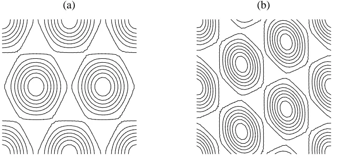
Fig. 1. Hexagonal patterns with wave integers (a) (2,1), (−2,1), (0,−2); (b) (3,0), (−2,−2), (−1,2).
Regular hexagons can however be obtained in a rectangular box if the ratio of the length of one side to the other is a multiple of √3; this choice has been used in numerical simulations to investigate the relative stability of rolls and hexagons [13].
Two examples of irregular hexagonal patterns are illustrated in Fig. 1. In each case the amplitudes of the three modes have been chosen to be real and equal, so that the function plotted is
w=
3
X
i=1
cos(2π(mix+niy)/L). (10)
Fig. 1 (a) shows the case where the wave integer pairs are (2,1), (−2,1) and (0,−2), in which four hexagons occur in the box, while the six-hexagon case with wave integers (3,0), (−2,−2), (−1,2) is shown in Fig. 1 (b). The former can occur with periodic or Neumann boundary conditions, but the latter can only occur with periodic boundary conditions. The six-hexagon pattern shown in Fig. 1 (b) has been found in numerical simulations of magnetoconvection in a compressible fluid by Weiss et al. (1996) [18].
[image:5.595.320.458.85.240.2]There is a simple relationship between the number of hexagons N in the periodic box and the wave integers. This is
N =|m1n2−m2n1|. (11)
From (4) it follows that any pair of the wave integers can be used in this formula. This result is demonstrated as follows: the planform function (10) is maximized when x and y obey
m1x+n1y=pL, m2x+n2y=qL, (12)
wherep andq are integers. From (4) it follows that m3x+n3yis then also an integer multiple of L, so that w takes its maximum value of 3, corresponding to the centre of a hexagon. These equations give the lattice of points at which centres of hexagons occur. Three points on this lattice are
(a) p= 0, q= 0, x= 0, y= 0;
(b) p= 1, q= 0, x=n2L/(m1n2−m2n1), y=−m2L/(m1n2−m2n1) ; (c)p= 0, q= 1, x =−n1L/(m1n2−m2n1), y=m1L/(m1n2−m2n1) . These three points form a triangle that connects the centres of three hexagons. The area of this triangle is
|(n2,−m2)×(−n1, m1)|L2/2(m1n2−m2n1)2 =L2/2|m1n2−m2n1|,(13)
using the formula for the area of a triangle in terms of the cross product of two vectors. This area is half the area associated with each hexagon, since each triangle connects three hexagons but each hexagon is connected to six triangles. Dividing the total area of the squareL2 by the area of each hexagon gives the formula (11) for the total number of hexagons in the box.
To describe these hexagonal patterns it useful to have a parameter measuring how close the pattern is to regular hexagons. One such parameter is H = (k2
max−kmin2 )/kmax2 where kmax and kmin are the maximum and minimum of the three wavenumbers; ifH is small, the pattern is close to regular hexagons. Table 1 lists all hexagonal patterns in whichH <0.45 andN <25, giving the wave integers, the parameterH, the number of hexagonsN and the symmetry for each.
3 Nonlinear dynamics of hexagonal patterns
m1 n1 m2 n2 m3 n3 H N Symmetry
2 1 -2 1 0 -2 0.20000 4 Y
3 0 -2 2 -1 -2 0.44444 6 N
3 1 -1 -3 -2 2 0.20000 8 Y
3 2 -3 1 0 -3 0.30769 9 N
4 1 -3 2 -1 -3 0.41176 11 N
3 3 -4 0 1 -3 0.44444 12 N
4 0 -2 -3 -2 3 0.18750 12 Y
4 2 -1 -4 -3 2 0.35000 14 N
3 3 -4 1 1 -4 0.05556 15 Y
4 2 -4 2 0 -4 0.20000 16 Y
4 3 -4 1 0 -4 0.36000 16 N
5 1 -2 -4 -3 3 0.30769 18 N
5 2 -4 2 -1 -4 0.41379 18 N
5 1 -4 3 -1 -4 0.34615 19 N
5 0 -3 -4 -2 4 0.20000 20 Y
5 2 -5 2 0 -4 0.44828 20 Y
5 2 -2 -5 -3 3 0.37931 21 Y
5 3 -1 -5 -4 2 0.41176 22 N
5 2 -1 -5 -4 3 0.13793 23 N
4 4 -5 1 1 -5 0.18750 24 Y
6 0 -3 -4 -3 4 0.30556 24 Y
6 0 -4 -4 -2 4 0.44444 24 N Table 1
Wave integer combinations that generate hexagonal patterns. The parameter H
measures the departure from regular hexagons and N is the number of hexagons in the periodic box. The final column indicates whether or not the pattern has a reflection symmetry.
for a finite box sizeL, only discrete wavenumbers given by (3) can occur, and in general these will not includek0. For large values of L however, wavenum-bers close tok0 will be included, and the separation between wavenumbers in the vicinity of k0 scales as 1/L2. This allows a small parameter to be intro-duced, representing the difference betweenk0 and the three wavenumbers that generate the hexagonal pattern. With the scalingki =k0+O() fori= 1,2,3, the corresponding values of rc are rci =ro +O(2), since r
0 is the minimum of rc(k). Writing r =r0 +2r2, all growth rates are O(2) so the appropriate time scale for the amplitude equations is T =2t.
It is now possible to write down the governing amplitude equations for the three Fourier modes obeying the resonance condition (4). Writing
w=
3
X
1
Ajexp(2πi(mjx+njy)/L), (14)
it can be shown that the sum of the phases of the Aj tends to zero [12], so that with an appropriate choice of origin the amplitudes Aj can be taken to be real. The scaled amplitude equations are then
˙
A1=λ1A1+A2A3, ˙
A2=λ2A2+A1A3, (15)
˙
A3=λ3A3+A1A2.
Here, the dot represents the rate of change on the slow timescaleT, the linear coefficients λ1, λ2 and λ3 are proportional to (r−rcj)/2 and the amplitudes Ai have been scaled by a factor 2. With these scalings, all terms in (15) are of the same order, and any cubic terms in the amplitude equations will be smaller by a factor 2.
Note that the coefficients of the quadratic terms in (15) are equal. This is because (15) represents a small perturbation from the case of regular hexagons. The coefficients of the quadratic terms can be set to 1 by scaling the amplitudes Aj appropriately.
The dynamics of the system (15) depends crucially on whether there are any additional symmetries. It is useful to begin by briefly reviewing the well-known case of regular hexagons, for whichλ1 =λ2 =λ3. In this case the fixed points of (15) are the solution A1 = A2 = A3 = 0, which is stable for λ1 < 0 and unstable for λ1 > 0, and four equivalent hexagonal solutions A1 =±λ1, A2 =±λ1, A3=−A1A2/λ1, for which the three eigenvalues are 2λ1, 2λ1 and
In the case where λ1 = λ2, two of the wavenumbers are equal in magnitude and the resultant pattern has a reflection symmetry (e.g. Fig. 1a). The fixed points are
(i) A1 = A2 = A3 = 0. This is stable if λ1 < 0 and λ3 < 0, and undergoes stationary bifurcations at λ1 = 0 and λ3 = 0.
(ii) A1 = ±√λ1λ3, A2 = ±√λ1λ3, A3 = −A1A2/λ3. These four equivalent solutions only exist when λ1λ3 > 0. Its eigenvalues s obey s = 2λ1 or s2 − λ3s−2λ1λ3 = 0. The product of roots of this quadratic is negative so this solution can never be stable.
For the case where all three linear terms in (15) are different, the three wavenumbers are different and the hexagonal pattern does not have mirror symmetry (e.g. Fig. 1b). The fixed points are
(i) A1 = A2 = A3 = 0. This is stable if λ1 < 0, λ2 < 0 and λ3 < 0, with stationary bifurcations at λ1 = 0, λ2 = 0 and λ3 = 0,
(ii) A1 = ±√λ2λ3, A2 = ±√λ1λ3, A3 = −A1A2/λ3. Again there are four solutions of this type. This solution only exists when either λ1 < 0, λ2 < 0, λ3 < 0 or λ1 > 0, λ2 > 0, λ3 > 0. The eigenvalues s obey s3−(λ1 +λ2 + λ3)s2+ 4λ1λ2λ3 = 0. Since there is no linear term, the three eigenvalues obey s1s2+s2s3+s3s1 = 0 which shows that the solution can never be stable.
3.1 Amplitude equations including cubic terms
The analysis of the previous section, although asymptotically correct, has two drawbacks. Firstly, no stable nonlinear solutions are found, and secondly, solutions in the form of rolls (involving a single wavenumber only) are not found. These problems can be overcome by the addition of cubic terms to the amplitude equations. In general, this is inconsistent, since quadratic and cubic terms can only appear together if the amplitudes areO(1), in which case terms of all order should appear in the equations. However, a consistent scaling can be obtained if the asymmetry in the problem (and hence the quadratic term) is small; this is a commonly used assumption [1,7,10]. The appropriate scaling is that the coefficient of the quadratic term is O() (recall that is the scale of the difference between the wavenumbers). The growth rates are O(2) as before, and a consistent balance between linear, quadratic and cubic terms is obtained if the amplitude scaling isAi =O(). The scaled amplitude equations then become
˙
A1=λ1A1+A2A3−A1(A21+βA22+βA23) ˙
A2=λ2A2+A1A3−A2(A22+βA23+βA21) (16)
˙
It can be assumed that the quadratic and cubic terms are equal in each tion because the system (16) represents a small perturbation from the equa-tions for regular hexagons; any deviation appears at higher order. By choosing an appropriate scaling for both time and the amplitudes, the coefficients of the quadratic terms and the A3
i terms have been set to unity. The constant β is problem–dependent and cannot be scaled out. For simplicity it is assumed that β >1. This means that rolls are stable in the absence of the quadratic term. This is indeed the case for both Rayleigh–Benard convection and for the Swift–Hohenberg equation.
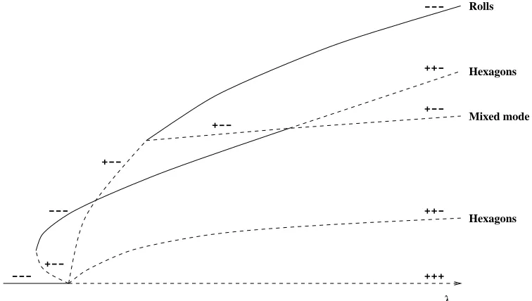
It is helpful to consider first the familiar case of regular hexagons for which λ1 = λ2 = λ3 [6]. The bifurcation diagram for this case is shown in Fig. 2. Solutions in the form of rolls (e.g. A1 = ±√λ1, A2 = A3 = 0) are stable for λ1 >1/(β−1)2. Hexagons (withA1 =A2 =A36= 0) appear at a transcritical bifurcation from the trivial solution where they are unstable, but gain stability though a saddle–node bifurcation at λ1 =−1/(4 + 8β) = λSN and are stable for λSN < λ1 < λTR = (β+ 2)/(β−1)2. There are two regions of overlapping stable solutions and hence hysteresis; forλ1small and negative both the trivial solution and hexagons are stable, while for larger λ1 both hexagons and rolls are stable. The rolls and hexagons are linked via a branch of mixed modes (e.g. A1 =A2 6= A3) which are always unstable. The upper stability boundary of hexagons atλ1 =λTR occurs at a transcritical bifurcation withD3 symmetry, where the hexagons and mixed modes have a double zero eigenvalue; a centre manifold reduction near this point yields the normal form
˙
x=µx+x2−y2, y˙ =µy−2xy (17)
with the symmetries of rotation through 2π/3 and reflection y → −y. This system is discussed in more detail later.
The procedure for analysing (16) is similar to that for (15). The behaviour de-pends on whether or not any ofλ1,λ2 andλ3 are equal, so these two cases are studied separately. Since the equations (16) have been considered by other au-thors [12,7], the details of the calculations are not given. Attention is focussed on points not described by the previous work. The case of symmetric patterns with two equal wavenumbers is described in section 3.2 and the asymmetric case with three different wavenumbers is discussed in section 3.3.
3.2 Patterns with two equal wavenumbers
The fixed points of (16) when λ1 =λ2 are as follows.
---
+-- ++- +--
++-
+--λ
---+++
---
+--Rolls
[image:11.595.102.480.70.284.2]Hexagons Mixed mode Hexagons
Fig. 2. Bifurcation diagram for regular hexagons. Solid lines indicate stable solutions and dashed lines represent unstable solutions. Pluses and minuses show the signs of the three eigenvalues of each branch.
(ii) ‘λ1-rolls’ with A1 = ±√λ1, A2 = A3 = 0; or A2 = ±√λ1, A1 = A3 = 0. These rolls are appear at a supercritical pitchfork bifurcation and are stable if λ1 >(1−λ3+λ3β)/β(β−1).
(iii) ‘λ3-rolls’ with A1 = A2 = 0, A3 = ±√λ3. These rolls also bifurcate supercritically, are stable if λ1 < βλ3 −√λ3, and have bifurcations at λ1 = βλ3±
√
λ3.
(iv) A mixed mode which can be regarded as hexagons, for whichA1 =±A2. This solution also branches from the zero solution at a pitchfork bifurcation at λ1 = 0, which is supercritical if 1 +β+ 1/λ3 > 0. At onset, A3 is much smaller than A1 and A2, so this pattern has a rectangular appearance. This solution can undergo saddle-node bifurcations, and branches from theλ3-rolls at λ1 =βλ3 ±
√
λ3.
(v) A mixed mode in which all the amplitudes are different. This solution branches from theλ1-rolls at λ1 = (1−λ3+λ3β)/β(β−1), and can never be stable.
To draw the bifurcation diagram, the number of parameters can be reduced to one by supposing that β and the box size L are fixed but r is allowed to vary. This is equivalent to writing λ1 = λ3 +δ, with δ fixed. There are two possible cases, according to the sign of δ, and these are shown in Fig. 3 and Fig. 4. In the bifurcation diagrams it is assumed that δ is small, so that the bifurcations from the zero solution are close together.
--- Rolls
+--
---
+--Different
Equal
Equal
++-λ
Equal
+--Rolls
+++
---Fig. 3. Bifurcation diagram for hexagons with mirror symmetry in the case where the double mode bifurcates first (δ > 0). The mixed modes are labelled according to whether all three amplitudes are different, or two are equal.
Equal
λ
++- --- Rolls
+--Equal +--
++-+-- +-- Different
Equal
+--
---Rolls
+++
---Fig. 4. Bifurcation diagram for hexagons with mirror symmetry in the case where the single mode bifurcates first (δ <0).
bifurcation. Forδ >1/(1 +β), the mixed mode bifurcates supercritically. This mixed mode loses stability when it bifurcates to the (unstable) solution with all amplitudes different. Both roll solutions become stable at largeλ1.
[image:12.595.105.478.68.281.2] [image:12.595.104.477.340.553.2]and rejoins the roll branch, at which point the rolls regain stability. For larger values of|δ|the region of stable mixed modes decreases and forδ <−1/4(β−1) there are no stable mixed modes, so that rolls are always stable.
It is of interest to note that these diagrams can be determined to a considerable extent just by considering the splitting of the hexagonal case (Fig. 2) induced by the symmetry-breaking. The single branch of rolls splits into two branches, and both hexagon branches become mixed modes withA1 =±A2. The mixed mode with A1 = ±A2 is unaltered, while that with A1 = ±A3 becomes a mixed mode with all amplitudes different. It follows that in both the cases δ > 0 and δ < 0, at large λ1 there must be two stable roll solutions, three mixed modes withA1 =±A2 (two with a ++−stability and one with +−−), and one mixed mode with all amplitudes different. This approach can be used to construct Figs. 3 and 4 except nearλ1 = 0, where the amplitudes are small, and nearλ1 =λTR = (β+ 2)/(β−1)2. Near this latter point, where in the case of regular hexagons there is a transcritical bifurcation (17) withD3 symmetry, the rotational symmetry is broken, but the reflection symmetry (y→ −y) is retained. A centre manifold reduction of (16) nearλTR for smallδleads to the normal form
˙
x=µx+x2−y2−δ, y˙ =µy−2xy, (18)
where µ is proportional to λ1−λTR and xand y are rescaled forms of 2A3− A1 −A2 and A1 −A2 respectively. In the case of regular hexagons (δ = 0) three mixed modes cross through the hexagons as µ passes through zero and the phase portraits are as shown in Fig. 5(a). For δ 6= 0 the behaviour of (18) depends on the sign of δ. Forδ > 0, two pitchfork bifurcations occur at µ=±2qδ/3 and the sequence of phase portraits is as shown in Fig. 5(b). For δ <0, two saddle-node bifurcations occur atµ =±2√−δ; the phase portraits are shown in Fig. 5(c). This analysis enables the correct connections to be made to the various branches in the Figs. (3) and (4).
3.3 Patterns with three different wavenumbers
In the case where the pattern involves three different wavenumbers,λ1,λ2 and λ3 are all different. The fixed points of (16) are:
(i) A1 = A2 = A3 = 0. This is stable if λ1 < 0, λ2 < 0 and λ3 < 0, and undergoes stationary bifurcations at λ1 = 0, λ2 = 0 and λ3 = 0.
(ii) Three branches of rolls, for exampleA1 =±√λ1, A2 =A3 = 0. These are stable if λ1+λ2 <2βλ1 and (λ2−βλ1)(λ3−βλ1)> λ1.
(a)
(b)
[image:14.595.102.486.70.401.2](c)
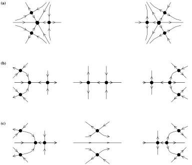
Fig. 5. The splitting or ‘unfolding’ of the transcritical bifurcation with broken D3
symmetry (18). Phase diagrams are shown withµincreasing from left to right, for the three cases: (a)δ= 0: Three mixed modes cross through the hexagons. (b)δ >0: Two mixed modes with all amplitudes different disappear at a pitchfork bifurca-tion with a mixed mode with two amplitudes equal, then reappear at a pitchfork bifurcation with the other mixed mode. (c) δ <0: The two mixed modes with two amplitudes equal disappear and then reappear at two saddle-node bifurcations.
With a fixed box size, we can setλ1 =λ2+α=λ3+δwithαandδfixed. Since the three modes are equivalent, it can be assumed without loss of generality that δ > α > 0, so that the rolls bifurcate in the order A1, A2, A3 as λ1 increases. The following results can then be obtained for the roll solutions: The first branch of rolls to bifurcate is stable at onset. For small α and δ these rolls lose stability and then regain stability as λ1 increases; for larger α and δ these rolls are always stable. The second branch of rolls to bifurcate is unstable at onset and becomes stable at a bifurcation to a mixed mode. The third branch of rolls is also unstable at onset, has two bifurcations to mixed modes and is then stable.
+--λ
Rolls
+--
---
++- +--
---Rolls Rolls
+++
---Fig. 6. Bifurcation diagram for hexagons without mirror symmetry.
the transcritical bifurcation at λ1 =λTR a centre manifold reduction yields a second-order system analogous to (18):
˙
x=µx+x2−y2−γx, y˙ =µy−2xy−γy. (19)
Here, both the rotation and reflection symmetries have been broken. The constants γx and γy are related to α and δ but their value is not important. The behaviour of (19) is similar to that shown in Fig. 5(c) (but without the mirror symmetry), so that two of the mixed modes undergo a pair of saddle-node bifurcations, while two undergo no bifurcations, as shown in Fig. 6.
4 Numerical simulations of the asymmetric Swift–Hohenberg equa-tion
To illustrate the results of the preceding work, this section describes numerical simulations of the Swift–Hohenberg equation [17] modified by the addition of a quadratic term:
∂w
∂t =rw−(1 +∇
2)2w+sw2−w3. (20)
[image:15.595.102.486.70.288.2](a) (b)
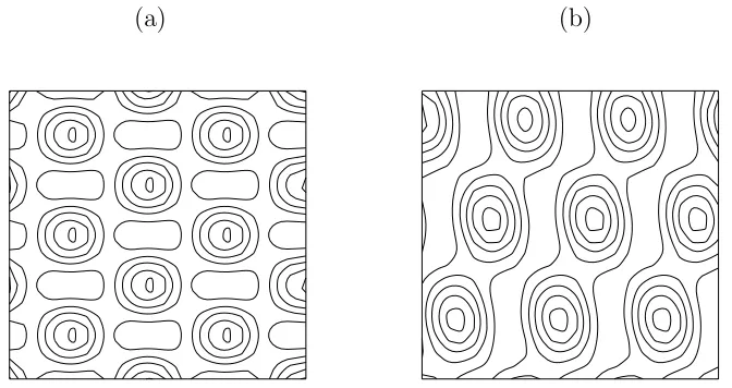
Fig. 7. Numerical solutions to (20) withs= 0.25. (a)r= 0.03,L= 23, showing 12 irregular hexagons. (b) r= 0.05,L= 21.25, showing 9 irregular hexagons.
substituting three Fourier modes of the form (14) into (20), the amplitude equations (16) are obtained with β = 2 andλi = 3(r−(1−k2
i)2)/4s2.
A Fourier spectral method was used to solve (20) with periodic boundary conditions in the region 0 < x, y < L. In Fourier space the linear parts of (20) can be solved exactly since the Fourier modes decouple. The nonlinear terms were integrated using the second-order Adams–Bashforth method. The initial condition chosen was a small-amplitude random perturbation to the zero solution.
For the case of hexagons with reflection symmetry, the pattern with 12 hexagons with wave integers (4,0), (−2,3) and (−2,−3) was studied. In this case, there are two different possible bifurcation diagrams (Figs. 3 and 4) according to whether the double mode or the single mode bifurcates first. For L= 23, the (−2,3) and (−2,−3) modes bifurcate first and therefore the appropriate bi-furcation diagram is Fig. 3. However for these parameters, δ= 0.445, so from the analysis of section 3.2 we expect the bifurcation to irregular hexagons to be supercritical. The numerical results show 12 hexagons for 0.002≤r≤0.03 and pure (3,2) rolls for r≥0.05, with both solutions stable forr= 0.035 and r= 0.04. This is consistent with Fig. 3. The solution forr= 0.03 is shown in Fig. 7(a).
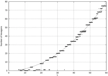
[image:16.595.318.455.102.243.2]0 10 20 30 40 50 60 70 80
0 10 20 30 40 50 60
Number of hexagons
[image:17.595.101.478.74.339.2]L
Fig. 8. Number of hexagonsN against box sizeLfor the equation (20) withr= 0.02 and s= 0.25.N = 0 indicates that the zero solution is stable and N = 1 indicates that rolls are stable. The dashed line is the curve N = √3L2/8π2, obtained by dividing the area of the box by the area of a regular hexagon.
The solution with 9 hexagons, involving the wave integers (3,2), (−3,1) and (0,−3) was chosen to study the case without reflection symmetry. This so-lution was found when the box size L was 21.25, and at this value of L the (−3,1) mode bifurcates first. A solution with 9 hexagons was found for 0.02 ≤r ≤ 0.055 and rolls with wave integers (3,1) were found for r ≥ 0.06. For r = 0.057 both solutions were found to be stable. Referring to the bifur-cation diagram (Fig. 4), rolls are also expected for small r; in fact however a hexagonal solution with 8 hexagons was found for r ≤ 0.02. Interactions between hexagonal patterns with different numbers of hexagons are of course beyond the scope of the analysis of section 3. The solution for r = 0.05 is shown in Fig. 7(b).
condition in each case. Values of L between 6 and 60 were used, with a step of 0.25 in L. The results are summarised in Fig. 8, which plots the number of hexagons against the box size. Where the number of hexagons is zero this indicates the zero solution, and a solution in the form of rolls is shown as one hexagon. Note that there are regions in which both rolls and hexagons are stable, and also regions in which two or even three different types of hexagons are stable.
Of the hexagonal solutions in table 1, those with 4, 8, 9, 12, 15, 16, 20, 23 hexagons were found. Note that, as might be expected, these are the solutions with low values of H, i.e. those that are closest to regular hexagons. There appears to be a preference for the symmetric hexagons. However this is no longer true at large values of the box size, where there are roughly as many asymmetric patterns as symmetric ones.
5 Conclusions
The main results of this paper are as follows. For numerical experiments with periodic boundary conditions, or laboratory experiments with Neumann boundary conditions, a perfectly regular hexagonal pattern is not permitted in a square box or any box with rational aspect ratio. Instead, patterns of irregular or ‘non-equilateral’ hexagons are observed. These patterns are com-posed primarily of three wavenumbers, and occur in two types. If two of the wavenumbers are equal then the resulting pattern has a mirror symmetry, but if all the wavenumbers are different it does not. There is a simple relation-ship (11) between the number of hexagonal cells in the pattern and the three wavenumbers.
The nonlinear dynamics of these patterns is controlled by the amplitude equa-tions (16). The results of the analysis of these equaequa-tions are summarised in the bifurcation diagrams of Figs. 3, 4 and 6. These provide a more complete picture of the dynamics than has been given by previous studies of the equa-tions [1,7,8,12]. A useful technique for clarifying the bifurcaequa-tions that occur is the centre manifold reduction near the transcritical bifurcation withD3 sym-metry. This reduces the algebra of the analysis considerably, enabling firm conclusions to be drawn regarding the connections between different solution branches.
be-haviour and a preference for three-dimensional patterns over two-dimensional rolls.
This work was motivated by numerical simulations of compressible magne-toconvection [18], in which hexagonal patterns with six rising plumes were found. The results obtained suggest that for very small Rayleigh numbers, rolls should be stable, and that for larger Rayleigh numbers rolls should again become stable. However it must be borne in mind that the equations (16) are only valid if the up–down asymmetry (the departure from the Boussinesq approximation in the case of convection experiments) is small, and this is generally not the case. There is much more complicated dynamics in these numerical experiments and further analytical work is required to understand and interpret them fully.
Acknowledgements
I am grateful to the University of Nottingham, the Royal Society and the Nuffield Foundation for financial support. This work has benefited from dis-cussions with S. Cox, M. Proctor, A. Rucklidge and N. Weiss.
References
[1] S.M. Cox, IMA J. Appl. Mathematics (1997).
[2] J.D. Crawford, Phys. Rev. Lett 67(4) 441–444.
[3] J.D. Crawford and E. Knobloch, Ann. Rev. Fluid Mech 23 (1991) 341–387.
[4] J.D. Crawford, J.P. Gollub and D. Lane, Nonlinearity 6 (1993) 119–164.
[5] B. Dionne, M.Silber and A.C. Skeldon, Nonlinearity, in press.
[6] M. Golubitsky, J.W. Swift and E. Knobloch, Physica D 10 (1984) 249–276.
[7] P. Hall and R.E. Kelly, Physical Review E 52 (1995) 3687–3696.
[8] R.B. Hoyle, G.B. McFadden and S.H. Davis, Phil. Trans. A 354 (1996) 2915– 2949.
[9] E.L. Koschmieder and S.A. Prahl, J. Fluid Mech. 215 (1990) 571–583.
[10] C. Kubstrup, H. Herrero and C. Perez-Garcia, Phys. Rev. E 54 (1996) 1560– 1569.
[12] B.A. Malomed, A.A. Nepomnyashchy and A.E. Nuz, Physica D 70 (1994) 357– 369.
[13] P.C. Matthews, M.R.E. Proctor and N.O. Weiss, J. Fluid Mech. 305 (1995) 281–305.
[14] Pattern Formation and Instabilities in Continuous Dissipative Systems, Physica D 97 (1996).
[15] M.R.E. Proctor and P.C. Matthews, Physica D 97 (1996) 229–241.
[16] A.C. Skeldon, K.A. Cliffe and D.S. Riley, J. Comp. Phys, in press.
[17] J. Swift and P. Hohenberg, Phys. Rev. A15, (1977) 319–328.